Keywords

SAR , Scatterometer , Polarimetry , Dielectric properties , Calibration , Modeling , Validation , Uncertainty

1 . INTRODUCTION

Soil moisture (SM) regulates inland water cycle, soil activities, atmospheric balance, vegetation cover, land degradation, human activities, etc. and therefore, important for sustainable land and climate change management (Sano et al., 2006; Pellarin et al., 2009; Bhagat, 2014; Das and Paul, 2015). It is an important variable for weather predictions (Jia et al., 2009), climate change modeling, surface runoff predictions (Sano et al., 2006; Kelly et al., 2003; Brocca, et al., 2010; Said et al., 2012), flood risk estimations (Schumann and Baldassarre, 2010), drought monitoring (Wanders et al., 2012), agricultural area mapping (Wang et al., 2010), crop modeling (Ines, 2013), irrigation management (Saindranath et al. 2000; Hajj et al., 2016; Said et al., 2012), etc. and highly varies with space and time, therefore high spatial and temporal resolution requires for realistic results from SM retrieval models (Wanders et al., 2012). In-situ sensors for SM measurements are costly and provide local information (Hajj et al., 2016). Land-surface models are unable to produce near-surface SM at local and regional scale (Pellarin et al,. 2009; Jia et al., 2009).

Remote sensing (RS) techniques provide spatial distribution of SM from few squire meters to kilometers, which not requires areal averaging from point data (Wagner et al., 2007). Space-borne passive microwave remote sensing of SM is not adequate for requirements of studies at watershed, catchment, and field scale with analyses at finer scale spatial resolution (Das et al., 2008; Tomer et al., 2015). However, radar backscatter has significant, strong, positive, linear and independent relationship with volumetric SM (0-5cm depth) (Shoshany et al., 2000; Romshoo and Musiake, 2003; Jia et al., 2009). Therefore, space-borne active microwave sensors like SAR (Table 1) are more useful to meet the requirements of spatial resolution for SM analyses at small-scale land surface units i.e. watershed, catchment area, agricultural fields, etc. (Verhoest et al., 2008; Tomer et al., 2015; Hajj et al., 2016; Filion, et al., 2016).

SM retrievals using active microwaves space based sensors are very attractive for meteorological: climatological analysis (Zribi et al., 2011), weather forecasting, drought analyses; hydrological: runoff estimations (Brocca et al., 2010), flood studies, wetland detection (Dwivedi et al,. 2000); agronomic: agricultural productivity predictions; human health analysis; national security analysis, etc. (Alvarez-Mozos et al., 2008; Entekhabi et al., 2010). Scholars have reported better results of SM retrievals from active sensors than the passive sensors (Wanders et al., 2012). SM estimations are: 1) more realistic for near surface retrievals (Pellarin et al., 2009; Wanders et al., 2012); 2) relatively unaffected by cloud cover: atmospheric water and hydrometeors for microwave backscatter (Kelly et al. 2003); 3) change detection from dry (0%) to very humid (100%) soils (5cm deep) (Djamai, et al., 2015); 4) possibilities of finer scale, field level estimations and variation analysis (Romshoo and Musiake, 2003; Das and Paul, 2015); and 5) useful for SM analysis over irrigated areas (Hajj et al., 2016).

Radar backscatters are sensitive to land surface characteristics including the dielectric constant (Gorrab et al., 2015) and surface roughness (Root Mean Square (rms) height and correlation length) of the soil (Zribi and Dechambre, 2003), and the physical and geometrical properties of vegetation (vegetation water content, backscatter size, shape, orientation, etc.) (Srivastava et al., 2015), the local incidence angle (Braun and Hochschild, 2017), frequency and polarization (Patel et al., 2006). SM can be detected and delineated using different methods and techniques reported in the literature (Zribi and Dechambre, 2003; Du et al., 2010) are: (a) quantitative measurements of SM for bear soils using polarized SAR data- 1) dual-polarization e.g. L-band SAR data (Dubois et al., 1995) (2) three-polarization SAR measurements (Oh et al., 1992), (b) multi-incidence angle SAR data for correcting the effects of surface roughness, (c) combination of optical data and SAR measurements for correcting vegetation effects, (d) change detection of SM using repeat SAR data; (e) Bayesian method of soil moisture estimations, (f) combination of active microwave data and passive microwave data. Thus, 1) finer spatial resolution, 2) multiple satellite sensors, 3) strong relation to , 4) penetration up to ~5cm depth, and 5) insensitive to clouds and 6) less sensitive to atmospheric condition including smoke, fog, rain, snow, etc. (Yue et al., 2016) are commonly reported advantages of the radar sensing of SM (Moran et al., 2004).

Scholars like Verhoest et al. (2008), Wang and Qu (2009), Barrett et al. (2009), Das and Paul (2015), etc. have reviewed scholarly literature on SM retrievals using active MW sensors. Verhoest et al. (2008) have summarized the problems encountered when parameterizing soil roughness and impact of the errors made on the retrieved soil moisture and noted need of more studies on the uncertainty assessment of SM retrieval models. Wang and Qu (2009) have reviewed applications of satellite based active microwave remote sensing (AMWRS) of surface SM. Barrett et al. (2009) have reviewed the current status to highlight the key areas for research in SM retrievals using active MW remote sensing data. Das and Paul (2015) also have reviewed research reports on SM retrieval using active MW remote sensing data and different models. Ouchi (2013) has reviewed recent trends and development of SAR with related techniques, selected topics and applications. Further, this study focussed on review the applicability to models available for SM retrievals to outline the trends and scope for further studies.

2 . SPACE-BORNE ACTIVE MICROWAVE REMOTE SENSING

Active microwave remote sensors like SAR have capacity to get high resolution images during day-night time in all-weather conditions (Ouchi, 2013) however, microwaves are very sensitive to geometric conditions at surface like topography, soil texture, surface roughness, vegetation cover, SM, etc. (Blumberg et al., 2002; Walker et al., 2004; Sanli, et al. 2008). Active sensors (e.g. SAR) offer SM data at higher spatial resolution compared to passive sensors (Kong and Dorling, 2008). Wanders et al. (2012) reported more realistic performance of ASCAT than AMSR-E and SMOS for estimation of actual near-surface SM over Spain. SAR data relatively unaffected by cloud cover including atmospheric water and hydrometeors for microwave backscatter at 5.3GHz (Kelly et al., 2003).

There are two active microwave main sensor types: 1) synthetic aperture radar (SAR) and 2) scattermeters. We have several advanced space borne SAR sensors (Table 1) (Kong and Dorling, 2008; Du et al., 2010; Ouchi, 2013). Popular approaches of SAR data used for SM retrievals are (Blumberg et al., 2002): 1) time series, 2) quad-polarized, and 3) multiple-look angle.

The backscattering coefficient of ERS-2 SAR data shows high sensitivity to surface SM at a field scale (Romshoo and Musiake, 2003). Airborne SAR data captured at an incidence angle between 10º and 20º and C-band frequencies are suggested for SM monitoring therefore, theoretically ERS-1 SAR is an ideal SM sensor as they are capturing the data at incidence angle of 23º, and C-band, 5.3GHz frequency at VV -polarization with 30m spatial resolutions (Kelly et al., 2003). The ERS SAR data is single polarized and single frequency. Therefore, multiple look scenes have been used in different studies to solve the parametric problems: more sensitive to surface roughness and less to the dielectric properties (Blumberg et al., 2002).

The new ENVISAT Advanced Synthetic Aperture Radar (ASAR) Wide Swath Mode (WSM) data (single-frequency (C-band), single-polarization (VV)) provide good potential for routinely monitoring near surface SM due to the increased temporal revisit capability compared with ERS2 SAR (Kong and Dorling, 2008). ASAR can be operated in different modes i.e. 1) Narrow Swath modes at high resolution (30 m) and 2) Wide Swath modes at medium resolution (150 m) with temporal revisit capability of 3–5 days, area coverage of 400  400 km and resolution of 1km. Walker et al. (2004) have used C-band vertically polarized SAR data captured using Second European Remote Sensing (ERS-2) satellite to estimate SM in surface layer. Zribi et al. (2011) have estimated SM for evaluation of soil evaporation using ENVISAT-ASAR images over semi-arid region in North Africa. ASCAT data expresses values between 0 and 100 for very dry and very wet conditions, respectively (Wanders et al., 2012). Further, Djamai et al. (2015) have estimated variation in SM for the top soil layer (5cm deep) using ASCAT from onboard the Meteorological Operational (MetOp). HJSAR carries S-band (3.2 GHz) has good penetration ability with \( P_{VV}\), 24 hours revisit period and 20m ground resolution (Du et al., 2010). Pellarin et al. (2009) have used AMSR and METEOSAT second generation (MSG) measurements for retrieval algorithm for the quality SM estimates.

Zribi and Dechambre (2003) have proved usefulness of RARDARSAT and ASAR-ENVISAT data captured using simultaneous dual incidence angle mode to characterize bare soil parameters. Kurucu et al. (2009) have fused Radarsat-1 fine beam mode image pertaining to the low lands with a satellite pour l’Observation de la Terre (SPOT)-2 satellite image of the same date for SM assessments for drought monitoring.

Aubert et al. (2013) have used TerraSAR-X data based on empirical soil moisture estimation logarithm for estimation of SM over agriculture area. Das and Paul (2015) have reported good potential of RISAT-1 images for the identification of local variations of soil dielectric constant (e), texture and SM. Gorrab et al. (2015) have used an empirical change detection approach using TerraSAR-X data and ground auxiliary PhetaProbe network measurements for SM estimations. Hajj et al. (2016) have developed an inversion approach to estimate surface SM over irrigated areas using SAR data (X-band). Further, Srivastava et al. (2015) have reported mapping abilities using SM retrieval models and multi-polarized SAR data without making any assumptions. However, little information is available about the applications of radar backscatter to estimate the SM distributions in transition zones between humid and semi-arid climates (Shoshany et al., 2000).

3 . RADIOMETRY

Radar backscattering coefficient can be expressed as (Narayanan et al., 1999): 1) soil dielectric properties and 2) soil roughness properties. Fundamental differences between passive and active microwave remote sensing are: 1) passive microwave remote sensors records emitted energy from soil in microwave, therefore depending upon soil microwave emissivity (Wigneron et al., 2003) and 2) active microwave sensors records backscattered energy from soil which was transmitted from same satellite therefore depending upon deference between amount of energy transmitted and received back.

3.1  Backscatter

Radar backscatters from soil surface show positive relation with near surface soil moisture (Blumberg et al., 2002) and roughness (Kong and Dorling, 2008). It decreases with increasing incidence angle and with decreasing roughness (Dubois et al., 1995). Microwave backscatter usually expressed as backscattering coefficient (\(\sigma ^{0}\)) (1) (Das and Paul, 2015). \(\sigma ^{0}\) demonstrates the combined effects of surface conditions (roughness and vegetation) and radar configurations (frequency, polarization, incident angle) (Kong and Dorling, 2008). It is the function, \(f\) of SM\( \theta _{S}\) and surface roughness.

\(\sigma ^{0}=f \left( h_{RMS},l \theta _{s} \right)\) after Rahman et al. (2008) (1)

Surface roughness can be modeled using the root mean squared height (\( h_{RMS}\)) and the correlation length (\(l\)) of the same height variation.

\(\sigma ^{0}\) is composition of three contributors (2) from vegetated surface:

\(\sigma ^{0}= \tau^{2} \sigma _{s}^{0}+ \sigma _{veg}^{0}+ \sigma _{int}^{0} \)   after Moran et al.(2004) (2)

where, \(\sigma ^{0}_s\) is backscatter from bare soil surface, \(\tau^{2}\) is two-way attenuation of the vegetation, \(\sigma ^{0}_{veg}\) is direct backscatter contribution of the vegetation and \(\sigma ^{0}_{int}\) is multiple scattering from the vegetation and ground surface (Moran et al., 2004). \(\sigma ^{0}_s\) has functional relationship (3) with SM,, \( V _{SM}\) as:

 \(\sigma _{s}^{0}=f \left( R,~V_{SM} \right)\)  after Moran et al. (2004)                               (3)

where, \(R\) is surface roughness term.

Further, Rahman et al. (2008) have suggested equation for estimations of \(l\) (4) and \( h_{RMS}\) (5) for parameterize IEM for preparation of surface SM map.

\(l= \omega \left( \Delta \sigma ^{0}, \sigma _{dry}^{0} \right)\)  after Rahman et al. (2008) (4)

\(h_{RMS}= \psi \left( \Delta \sigma ^{0}, \sigma _{dry}^{0} \right)\) after Rahman et al. (2008) (5)

where, \(\omega\) and \(\psi\) are functions determined by substitution of terms. Three radar images require for roughness mapping. Two images with different incidence angles for determination of \(\Delta \sigma ^{0}\) and one with dry ground condition for measurement of \(\sigma ^{0}_{dry}\). It can be calculated using two images captured in dry and wet conditions. The values of \(l\) and \( h_{RMS}\) can be substituted in the equation for \(\sigma ^{0}\) as (6):

\(\sigma _{wet}^{0}= \lambda \left( \Delta \sigma ^{0}, \sigma _{dry}^{0}, \theta _{S} \right) \)  after Rahman et al. (2008) (6)

here, subscript ‘wet’ in \(\sigma ^{0}_{wet}\) is used to distinguish it from backscatter of dry surface. This equation can be inverted (7) for estimation of surface SM as:

\(\theta _{S}= \lambda ^{-1} \left( \Delta \sigma ^{0}, \sigma _{dry}^{0}, \sigma _{wet}^{0} \right)\)after Rahman et al. (2008)  (7)

where, \(\Delta \sigma ^{0}\) and \(\sigma ^{0}_{dry}\) are function of roughness parameters as \(\Delta \sigma ^{0} \left( h_{RMS},l \right)\)  and \(\sigma _{dry}^{0} \left( h_{RMS},l \right)\).

The digital number (DN) of the ASAR data can be converted into radar backscattering coefficient,  \(\sigma _{i,j}\) (8) as:

\(\sigma _{i,j}=\frac{DN_{i,j}^{2}}{K}sin \left( \alpha _{i.j} \right)\)  after Rahman et al. (2008), Wang et al. (2010)                                               (8)

where, \(DN _{i,j}\) is the digital number of the pixel (\(i, j\)), \(a_{i, j}\) is the incidence angle, and \(K\)  is calibration constant.  

The polarized backscattering coefficient, can be expressed as:

\(\sigma _{VH}^{0}=\frac{k^{2}}{2}e^{2k_{z}^{2} \sigma ^{0}} \sum _{n=1}^{\infty} \sigma ^{2n} \vert I_{VH}^{n} \vert ^{2} \left[ \frac{W^{ \left( n \right) } \left( -k_{x},0 \right) }{n~!} \right]\) after Romshoo and Musiake (2004)                                           (9)

where, \(\sigma _{VH}^{0}\) is the polarized radar backscatter; \(V\)  and \(H\) are vertical and horizontal polarisation; \(k_{z}=\ k\ cos \theta \) and \(k_{x}=k\ sin \theta \), \(\sigma \) is surface \(rms\) height and \(W^{ \left( n \right) } \left( u,~v \right)\)  is the roughness spectrum of the surface.

Romshoo and Musiake (2004) have reported good agreement of estimation using the Dubois model for either no or sparse vegetation.

The radar backscatter (\(\sigma \)) of soil, with a range of moisture concentrations, can be approximated (10) as:

\(\sigma \left( dB \right) =aV_{sm}+b \)   after Shoshany et al.(2000)   (10)

where, \(a\)  and \(b\) are empirical coefficients and \(V_{sm}\) is volumetric SM.

Nonlinear relationship between backscatter volumetric SM observed for bare soils and linear relation is found over vegetated areas (Narvekar et al., 2015). Therefore, nonlinear models are useful for estimations of SM using backscatter coefficient on bear soil and linear over vegetated areas (see next sections).

Backscatter coefficient can be converted into dB using following equation (11):

\(\sigma _{dB}^{0}=10log_{10} \sigma ^{0}\) after Kong and Dorling (2008) (11)

For radar, co-polarized backscatter from earth surface is the product (12) of three components i.e. 1) soil surface backscatterer– two-way attenuation through a vegetation layer, 2) the backscatter from the vegetation and 3) the interaction between the vegetation and soil surface (Wang and Qu, 2009). Radars corporatized backscatter, \(\sigma _{pp}^{ \tau}\) is combination of three components (12):

\(\sigma _{PP}^{ \tau}= \sigma _{PP}^{s}~.exp \left( -2~.~ \tau_{c} \right) + \sigma _{PP}^{vol}+ \sigma _{PP}^{int}\)  Ulaby et al., (1996)  (12)

where, \(\sigma _{PP}^{s}\) is soil surface backscatter, \(\tau_{c}\) is two-way attenuation through a vegetation layer of opacity, \(\sigma _{PP}^{vol}\) is backscatter from the vegetation volume and \(\sigma _{PP}^{int}\) represents interaction between the vegetation and soil surface. Soil surface backscatter dominates the backscatter for bare surface and influenced by soil SM and surface roughness (Wang et al., 2009).

3.2  System Parameters

Parameters of microwave sensor are wavelength, polarization and incidence angle related to nadir (Schmugge, 1976).

3.2.1  Wavelength

X-band (shorter wavelengths, 3cm) reflects from canopy surface of vegetation, L-band (longer wavelengths, 24cm) penetrate through the canopy and reflect from the soil surface and C-band (intermediate wavelengths, 6cm) reflects from both the canopy and soil surface (Barrett et al., 2009). X- and L-band (TerraSAR-X, CosmoSkyMed and ALOS), and C-band with polarimetric data (RADARSAT-2) are widely suggested for better characterization of surface parameters (Verhoest et al., 2008). These bands provide data in combination of co-polarization (\( P_{VV},~P_{HH}\)) and Cross-polarization (\(P_{VH},~P_{HV}\)) (Table 1) and show exponential relationship with surface roughness over bare soil (Zribi et al., 2016). Therefore, many researchers have successfully used X- and C-bands to estimate the SM of bare soil with good results (Hajj et al., 2016). C-band (4-5GHz) penetrates into soil layer of 1-2cm, determines the composite reflection coefficient and sensitive to canopy. Further, Kaojarern et al. (2004) have reported potential depth of SM using C-band up to 10cm. This frequency can penetrate better into the dry vegetation canopy and at low incidence angles (Walker et al., 2003). C-band radar signals are directly dependent on the share of sand and clay in the soil. The sensitivity of radar signals to SM increases with decreasing soil clay content (Das and Paul, 2015). Zribi et al., (2007) have used C-band ASAR/ENVISAT for estimation of SM over bare soil with low-density vegetation and using data acquired at low-incidence angle. Further, Kaojarern et al. (2004) have been used C-band data for monitoring the SM in post-harvest rice field in Thailand. Kong and Dorling (2008) have estimated SM suing C-band, single-polarization (\(VV\)) images captured in descending mode and PCA technique. However, sensitivity of C-band to canopy makes difficult to separate SM induced scattering from rough soil surface including vegetation (Narayanan et al., 1999; Rötzer et al., 2015). It is difficult to map SM using C-band over vegetated area (Das et al., 2008) and discriminates between surface roughness is greater than 1.5cm (Baghdadi et al., 2008). C-band gives response to crop structure and foliage and L-band dependents vegetation characteristics like tree branch and trunk structures. L-band is useful to estimate SM up to 5cm in top soil layer and 20cm for uniform SM distribution in the profile and insensitive to short and modest vegetation cover as compared to SM and surface roughness (Narayanan et al., 1999). They penetrate through thin canopy layer of crops (Rahman and Sumantyo, 2012). C- and X-bands penetrate less in forested areas (Baghdadi et al., 2008). Therefore, L-band (1-2GHz) are the most promising techniques for SM retrievals (Das and Paul, 2015; Colliander, 2016) than the C- and X-bands. Scholars show better penetration capability in vegetation, relatively less sensitive to short and sparse vegetation and useful for detection and estimation of SM for agricultural as well as hydrological applications (Narayanan et al., 1999). L-band data with low incidence angles is suggested for minimization of the effect of vegetation and surface roughness. Further, \(\sigma _{HV}^{0}/ \sigma _{VV}^{0}\), signal (L-band) ratio are useful to distinguish bare soils from vegetation cover (Aubert et al., 2013). However, Baghdadi et al. (2008) have noted weak backscattering from wheat at X-band, and negligible at L- and C-bands.

X-band signals have equivalent potential to C-band for SM mapping (Baghdadi et al., 2008).  Aubert et al. (2013) have studied relationship between TerraSAR-X signals acquired at mono SAR configurations (incidence angle and polarization) and SM data for training database of 182 bare plots. Baghdadi et al. (2008) have suggested X-band for analysis SM ranges between 27% and 32%. Kirimi et al. (2015) used TerraSAR-X SM retrievals using the Oh Model. Further, Baghdadi et al. (2008) reported weak potential of this band for mapping the surface roughness.

Das and Paul (2015) have reported positive relationship of backscattering coefficient calculated for band RH and RV with volumetric moisture content in tropical dry and sub-humid zones in India. P-band penetrates into deeper soils but requires larger antenna and unmanageable from space-borne platforms (Narayanan et al., 1999).

L-band (0.3-3GHz) was used for the characterization of the dielectric constant for estimations of SM over arid soils (Gharechelou et al., 2015). The depth of microwave penetration in soil profile depends on wavelength and the complex dielectric constant of the soil. It can be express (13) as:

\(\delta p \cong \frac{ \lambda *\sqrt[]{ \varepsilon ^{'}}}{2 \pi * \varepsilon ^{"}}\)    Srivastava et al. (2015)   (13)

where, \(\delta p\) is depth of penetration, \(\lambda \) is wavelength, \(\varepsilon ^{'}\) is real part of complex dielectric constant; \(\varepsilon ^{"}\) is imaginary part of complex dielectric constant. Thus, L-, X-, and C-bands have potential of SM retrievals with in-depth knowledge of soil surface characteristics.  There is large contrast between the dielectric properties of soil and water. Backscatter increases with increasing water content in soil (Blumberg et al., 2002). However, shorter wavelength is relatively more sensitive to the surface roughness.

Figure modified after Das and Paul, 2015.

3.2.2  Polarization (P)

Radar backscatters depend on topography, soil texture, surface roughness and soil moisture (Walke et al., 2003) therefore, the data recorded using single configuration (polarization and incidence angle) is not sufficient for detection of SM specially under mature crops (Gherboudj et al., 2011). Radar data in multi-frequency, multi-polarization or multi-angle makes possible to separate the roughness, vegetation, topography, and soil moisture effects on recorded radar signals (Oh et al., 1992; Kong and Dorling, 2008).

The vertical polarization is more sensitive to SM than the horizontal polarization (Narvekar et al., 2015) and cross-polarized SAR data at longer wavelength has been suggested for the quantitative retrievals of vegetation (Patel et al., 2006). Microwave sensors (X-, L- and C-band) provide polarimetric data: co-polarized (\( P_{VV},~P_{HH}\)) and cross-polarised (\(P_{VH},~P_{HV}\)) data. The co-polarization backscattering coefficients are expression of nonlinear functions of the surface dielectric constant, the incidence angle, the wavelength and the root mean square of surface height (Wang 2009). Fully polarimetric data reduce ambiguity of the outcome (Kumar et al., 2017).

Cross-polarised (\(P_{VH},~P_{HV}\)) values are lower than the co-polarized (\( P_{VV},~P_{HH}\) values for magnitude therefore, more prone to errors (Narayanan et al., 1999). Co-polarized signals are less sensitive to vegetation, easy to calibrate and less susceptible to system noise (Das and Paul, 2015). Backscattering coefficient with \(P_{HH}\) is more sensitive to soil moisture than \( P_{HV}\). Therefore, \(P_{HH}\) and \( P_{VV}\) improve estimation of SMC (Baghdadi et al., 2015). Further, Zribi et al. (2007) have noted similar results \(HH\) and \(VV\) -polarizations. However, Gharechelou et al. (2015) have reported that \(HV\) -polarization is more sensitive to soil moisture than the \(HH\) over Aridic soils in Iran. Rahman and Sumantyo (2012) have used dual-polarized SIR-C and PALSAR backscatter data for forest analysis.

Cross-polarized data is more useful for analyzing the contribution of vegetation in the total backscattering (Necsoiu et al., 2013). Vertical polarization is less sensitive to vegetation coverage than the horizontal polarization (Jia et al., 2009).Vegetation strongly absorbs the signals in \(VV\) channel and \(HH\) is more sensitive for SM in near surface (Pasolli et al., 2014). Further, Bourgeau-Chavez et al. (2007) have reported that \(VV\)-polarization (ERS-2) is less sensitive than \(HH\)-polarization to the orientation of plant leaves. Du et al. (2010) have successfully used \(VV\)-polarisation at S-band of HJ SAR for SM retrievals. Therefore, \( P_{HV}\) removes the effect of vegetation and \(P_{HH}\) provides slightly better results than  (Holah et al., 2005). However, \(VH\) and \(HV\) are strongly correlated and give similar information (Pasolli et al., 2014). \(HH\) and \(HV\) channels of SAR are highly recommended to determine more precise estimations of SM (Holah et al., 2005; Pasolli et al., 2014).

PALSAR is reported as the most cost effective for providing data compared to ASAR versus RADARSAT at \(VV\) polarisation for better estimations of SM (Sanli et al., 2008). Further, Baghdadi et al. (2006) have recommended ASAR data at \( P_{VV}\) with more potential than RADARSAT-1 for SM estimation however, Sanli et al. (2008) found no better outputs. An inversion algorithm based on the co-polarized data will be more robust for vegetation and however, overestimate surface roughness and underestimate soil moisture (Dubois et al. 1995). Further, Baghdadi et al. (2013) have compared the fully polarimetric data at X-, C-, L-, P-, and UHF-bands and found no relevance of polarimetric parameters for characterization of the soil surface (moisture content and surface roughness) over bare agricultural areas. Therefore, more studies are required to find wide applicability of polarised data in different bio-physical units. 

3.2.3  Incidence Angle (θ)

Contribution of the backscattering from soil surface to the total backscattering mainly depends on the incidence angle (Hégarat-Mascl et al., 2002) and the characteristics of the vegetation. C-band energy penetrates through canopy with steep incidence angles over sparse vegetation (Bourgeau-Chavez et al., 2007). Therefore, incidence angle below 30º is recommended for retrieval analysis of SM content (Necsoiu et al., 2013, Filion et al., 2015). Moran et al. (2000) have used C-band, \(VV\) -polarized data captured at 23º incidence angle to minimize the influence diversity in terrain and vegetation. Hégarat-Mascl et al. (2002) show linear relationship of radar signal at \(VV\) -polarization and 23º incidence angle with SM. Sahebi et al. (2004) have used C-band with \(HH\) -polarization captured at 10°-12° incidence angle to minimise the roughness effect. Holah et al. (2005) have recommend low and medium incidence angles (20°-37°) as optimal parameter for SM estimations whereas the high-incidence angle (40°-43°) of ASAR images are the most suitable for roughness analysis with minimum influence of SM (Das and Paul, 2015). Therefore, SAR C-band images acquired at low (Patel and Srivastava, 2015) and medium incidence angle are suggested for the best SM estimations (Baghdadi et al., 2008). Various ranges as optimal incidence angle have been suggested for SM retrievals: 1) 10° to 20° (Romshoo and Musiake, 2004); 2) 10° to 17° (Patel and Srivastava, 2015), etc. However, Geng et al. (1996) have concluded that images captured at higher incidence angel gives larger difference between dry and wet soils for given polarisation. Moran et al. (2000) have noted importance of adjustment of topographic influence on local incidence angle. Bertoldi et al. (2014) have been used Standard Quad Polarization (\(HH\), \(HV\), \(VH\), \(VV\)) at mean incidence angle of 45 for SM retrievals over mountain area. Gorrab et al. (2015) have used TerraSAR-X image for mapping of bare soil surface parameters including SM.

Several studies have improved SM retrieval using SAR C-band images taken at two incident angles (Aubert et al., 2013). Zribi and Dechambre (2003) have used \(P_{HH}\) polarization of C band (5.3 GHz) acquired at two incidence angle 23º and 39º with 3 days delay to estimate SM using duel-configured integral equation model. They have proved usefulness of space-borne RARDARSAT and ASAR-ENVISAT data captured using simultaneous dual incidence angle mode to characterize bare soil parameters. Rahman et al. (2008) have suggested the method depends on radar images captured from two different view angles with the repeat cycle of the satellite. Simultaneously acquiring images at multiple polarizations and two view angles are useful to eliminate the errors due to registration inaccuracy (Rahman et al., 2008). Further, ratio of radar signals recorded at low to high incidence angle, \(\Delta \sigma ^{0} = \sigma_{26 ^{\circ} –28 ^{\circ}} \sigma_{50 ^{\circ} –52 ^{\circ}}\) decreases with surface roughness (Baghdadi et al., 2008). Co-polarization ratio increases with increasing incidence angle (Oh et al., 1992).

Santi et al. (2013) have used SAR data captured at various incidence angles (20° to 50°) for SM estimation using ANN. Das and Paul (2015) have used RISAT-1 signal with RH and RV configuration at high incident angle (48.11º) to analyse the behaviours of several soil conditions. Bai and He (2015) have not considered the effect of local incidence angle on the backscattered signal used for SM retrievals with help of Dubois model for the flat topography in prairie areas.

3.2.4  Radiometric Calibration (RC)

Sensor calibration requires for reliable results of the SM retrievals using SAR (Moran et al., 2000). Geng et al. (1996) have used Dobson method for relative calibration of single look, multi-polarized SAR image and reported 20% better results than non-calibrated data. Kelly et al. (2003) have reduced speckle using ‘adaptive Lee sigma filter’.  Method suggested by Laur et al. (1996) has been widely used for calibration (14) of SAR data (Shoshany et al., 2000; Kelly et al., 2003; Walker et al., 2003; Kaojarern et al., 2004; Said et al., 2012; etc.). 

\(\sigma ^{0}=DN^{2} \times \frac{1}{k}\frac{sinZ}{sinZ_{ref}}\) after Walker et al. (2003) (14)

where, \(k\) is the calibration constant,  \(Z\) is the zenith angle for the pixel, and \(Z_{ref}\) is reference incidence angle.

Bai et al. (2015) have used following equation (15) for radiometric calibration of TerraSAR-X image:

\(\sigma _{dB}^{0}=10~log_{10} \left[ \left( \vert k_{s} \vert ^{2}-NEBN \right) \times sin \left( \theta \right) \right]\) after Bai et al. (2015)  (15)

\(\sigma ^{0}\) is backscattering coefficient, \(\theta\) is incidence angle, \(k_s\) is calibration coefficient. \(k_s\) depends on \(\theta\)  and polarization. \(NEBN\) is noise equivalent beta naught, which interprets the noise contribution to the signals.

Scholars have been used algorithms developed by the German Aerospace Center (DLR) and the Italian Space Agency (ASI) for radiometric calibration of SAR images (Hajj et al., 2016). Radiometric calibration transforms the DN to a radar backscattering coefficient (16) for COSMOSkyMed (CSK) data.

\(\sigma _{i}^{0}=K_s~ \cdot DN_{i}^{2} \cdot sin \left( \theta \right) -NESZ\) after Hajj et al. (2016)   (16)

where, \(k_s\) is the calibration constant, \(\theta\) is the reference incidence angle, and \(NESZ\) is the Noise Equivalent Sigma Zero. Further, Hajj et al. (2016) have used following equation (17) for RC of CSK images

\(\sigma _{i}^{0}=DN_{i}^{2}~ \cdot ~\frac{1}{K~ \cdot F}~ \cdot sin \left( \theta \right) R_{ref}^{2~ \cdot R_{exp}}\)after Hajj et al. (2016)    (17)

where,\(R_{ref}\) is the reference slant range, \(R_{exp}\) is the reference slant range exponent, \(K\) is the calibration constant, and \(F\) is the rescaling factor. They have averaged these values, \(\sigma _{i}^{0}\) at plot level i.e. grassland plots in decibel scale using following equation (18):

\(\sigma _{dB}^{0}=10~ \cdot log_{10} \left( \sum _{}^{} \sigma _{i}^{0} \right)\)  after Hajj et al. (2016)   (18)

Kong and Dorling (2008) have used calibration procedure provided by data producer for calibration of ASAR data.

Topographic distortions are very difficult to remove from SAR image using calibration techniques because of layover and shadowing effects (Bertoldi et al., 2014). It makes more complexities for SM retrievals. Backscatter response varies according to soil types needs calibrations for each textural class. Further, SM moisture data has been also used for calibration of models which required for inversion of radar images (Baghdadi et al., 2006). Some scholars have used calibration curve prepared based on SM measurements according to soil types (Blumberg et al., 2002). However, some scholars have developed techniques for SM estimations without prior knowledge about roughness parameters with the help of calibration approach (Verhoest et al., 2008). Baghdadi et al. (2006) used calibration parameter dependent on roughness, the incidence angle (\(\theta\)), the polarization (\(P\)), and the radar frequency for replacement of in-situ SM data. Calibration based models are very sit-specific and not useful to extrapolate the SM for different bio-physical units. Thus, multiple frequency, - polarization, - incidence angle SAR images are suggested to remove surface roughness and vegetation effects from retrieved SM (Bourgeau-Chavez et al., 2007).

3.3  Surface Parameters

Radar backscatter has combined effect of: 1) surface conditions including slope, roughness, dielectric constant of the target e.g. SM and vegetation; and 2) radar configurations including frequency, polarization, incident angle (Kong and Dorling, 2008). The analysis of relationship between soil surface roughness and radar backscattering are important for precise SM estimations (Gorrab et al., 2015).

3.3.1  Surface Roughness

Surface roughness, \(Z_s\) is a description of the irregularity (randomness) of the micro-topography of the earth surface (Li et al., 2015). Roughness effect on radar backscatter is possibly equal to or greater than the effect of soil moisture (Lu and Meyer, 2002). Therefore, roughness parameterization is an important, crucial (Pant et al., 2010) and problematic issue in SAR-based soil moisture retrievals (Verhoest et al., 2008). The input data about roughness parameters for backscattering modeling needs for precise estimations of SM over bare surface (Zribi et al., 2005). It has been analyzed using two parameters: correlation length (\(l\)) and \(rms\) height (\(s\)) (Pant et al., 2010). Zribi et al. (2006) have analyzed role of roughness in surface scattering model for heterogeneous terrains. \(Z_s\) simply described (19) as:

\(Z_{s}=s^{2}/l\)  after Zribi and Dechambre (2003), Zribi et al. (2006)  19)

The variation of a surface height relative to reference surface for random component can be described using the standard deviation of surface height (\(s\)) and the surface correlation length (\(l\)). \(Z_s\) is key parameter in volumetric and spatial estimations of the SM using MW backscatters data. Many researchers have determined \(Z_s\) parameters, \(\sigma\) = 0.3–3cm, cl. = 3–35cm.

Researchers have developed the methods of \(Z_s\) retrieval using: 1) microwave backscatters from vegetation canopy, 2) triangular prisms, and 3) surface roughness testing apparatus and the corresponding testing methods. Further, Walker et al. (2003) have reported four methods for physically measurement of roughness parameters (1 to 2m length of profile): “(i) inserting a thin metal plate vertically into the soil and spraying with paint from horizontal direction; (ii) taking a photograph of the intersection of the ground surface with a gridded plate and digitizing the intersection; (iii) using a panel with drop pins; and (iv) using a laser profiler”. However, calculations of the  and the standard deviation of a surface height based three-dimensional parameters for the surface requires large efforts computation (Li et al., 2015). Li et al. (2015) have developed a GPU [Graphics Processing Unit]-based method to calculate the soil surface roughness parameters. Some scholars have used semi-empirical Water Cloud Model to eliminate the vegetation effects on the backscatter coefficient for SM estimations using, viz. Said et al. (2012) ERS-2 SAR images.

Long profiles are suggested for precise estimation of the roughness parameters (Verhoest et al., 2008) and direct measurement of roughness parameters over larger area is very time consuming and expensive (Pant et al., 2010). Therefore, SAR estimations of roughness parameters are suggested and many empirical models are available for these estimations. Oh et al. (1992) have calculated the polarization ratios for analysis of bare soil surface: co-polarized ratio, \(\sigma _{HH}^{0}/ \sigma _{VV}^{0}\) and cross-polarized ratio, \(\sigma _{HV}^{0}/ \sigma _{VV}^{0}\). Co-polarized ratio increases with incidence angle and increasing soil moisture content whereas cross-polarized ratio show weak dependence with soil moisture content. Further, Srivastava et al. (2008) have used depolarization ratios for estimations of surface roughness (20) using polarized Envisat-1 ASAR data as:

\(\sigma _{VH}^{0}- \sigma _{VV}^{0}\)  after Srivastava et al. (2008)    (20)

They have shown rms height from SAR backscatter as scatterplots using linear regression analysis (21; 22) as:

\(rms~height=A+B^{*} \left( \sigma _{VV}^{0} \right)\)after Srivastava et al. (2008)    (21)

\(rms~height=A+B^{*} \left( \sigma _{VH}^{0} \right)\)after Srivastava et al. (2008)    (22)

It is good indicator of surface roughness derived from multi-polarized SAR data.

\(C_{r}= \left( 1-\frac{L_{2}}{L_{1}} \right) \times 10\) after Das and Paul (2015)    (23)

where, \(C_r\) is roughness at any direction; \(L_1\) is the length of roller chain; and \(L_2\) is linear distance of chain due to roughness. Surface roughness using single SAR image of single band (C-band or X-band) can be represented (24) as:

\(\sigma =f \left( V_{sm}, \lambda \right) \Longrightarrow V_{sm}=f^{'} \left( \sigma \right)\) after Zhang et al. (2016)     (24)

where, \(\sigma\) is backscatter coefficient. Combined use of two bands of SAR images can eliminate the effect of surface roughness and establish relationship of  with volumetric SM. Zhang et al. (2016) have combined two SAR C- and X-bands using (25):

\(\begin{equation} \left.\begin{aligned} \sigma _{c}=f_{1} \left( V_{sm}, \lambda _{c} \right) \\ \sigma _{x}=f_{2} \left( V_{sm}, \lambda _{x} \right) \\ \end{aligned} \right\} {\implies} \ m_{v}=f^{'} \left( \sigma _{c}, \sigma _{x} \right) \end{equation}\)after Zhang et al. (2016)    (25)

Contribution of SAR backscatter for a vegetation cover depends upon the vegetation volume, dielectric and structure of the vegetation constituents as well as the frequency, polarization and incidence angle of the MW (Srivastava et al., 2015; Hajj et al., 2016). Many models are available for roughness estimations, however, no explicit model available for precise estimations. They are very site specific and confined to the study area. The radar-perceived roughness is a combination of surface and subsurface roughness.

3.3.2  Surface Correlation Length (\(l\))

Correlation length of surface provides reference to estimate the statistical independence of two points (Li et al., 2015). Accuracy of SM estimation using IEM model depends on measurements of correlation length (Baghdadi et al., 2006). However, measuring correlation length is pragmatic and difficult to interpret (Verhoest et al., 2008). The values are varied and depend on the length of transect and increasing with increasing profile length.

The correlation coefficient for radar detected scattering values spread over a 2D area can be calculated (26):

\(\sigma \left( j \right) =\frac{ \sum _{i=1,~k=1}^{M} \left( z_{i}-z_{i} \right) \left( z_{k}-z_{k} \right) }{ \sum _{i=1,}^{M} \left( z_{i}-z_{i} \right) } \vert \sqrt[]{ \left( x_{i}-x_{k} \right) ^{2}- \left( y_{i}-y_{k} \right) ^{2}} \epsilon \left( j-0.5,~j+0.5 \right)\)after Li et al. (2015)  (26)

where, \(j\) is the value gives to calculate the different correlation coefficients. Li et al. (2015) have recommended this method for calculation of the soil backward scattering coefficient using Advanced Integrated Equation Model (AIEM) of microwaves for ground detection.

Smoother profiles need longer profiles for the estimation of the correlation length (Callens et al., 2006). rms height does not decrease with increasing profile length therefore many profiles required to get precise estimations of the average correlation length.

3.3.3  Autocorrelation Function (ACF)

Autocorrelation function for lags,  \(\xi =j \Delta x \) (\(\Delta x \) is spatial resolution of the profile) of surface height is one of the surface roughness parameters (Barrett et al., 2009). Analytical models based on physical approximations require knowledge of the autocorrelation function (Vannier and Taconet, 2014). Bi-dimensional autocorrelation function more appropriate to characterize bare soil agricultural surfaces for multi-scale processes (Vannier and Taconet, 2014).

The Gaussian and exponential autocorrelation function have been widely used backscattering models for SM retrievals (Callens et al., 2006):

Gaussian function (27):

\(ACF \left( \xi \right) =e^{- \vert \xi \vert /l}\) after Verhoest et al. (2009)    (27)

Exponential autocorrelation function:

\(ACF \left( \xi \right) =e^{- \xi ^{2}/l}\) after Verhoest et al. (2009)   (28)

Exponential ACF shows smaller correlations at small lags than Gaussian function (Verhoest et al., 2009) therefore, Baghdadi et al. (2015) found better SM simulation with exponential autocorrelation function than with Gaussian function. Gaussian and exponential ACF differently describe the surface according to lags and correlation length. Gaussian ACF shows a smoother surface than the exponential for lags smaller than correlation length (Verhoest et al., 2009). The shorter the ACF indicates the smaller the correlation length (Callens et al., 2006). Exponential function produces ACF close to natural soils and Gaussian ACF to rougher surfaces (Callens et al., 2006). Therefore,  Ji et al. (1996) have used hybrid, Gauss-Exp function product of Gaussian and exponential ACF reported as a suitable model. Baghdadi et al. (2008) have computed rms surface height and correlation length for each training field using the mean of the autocorrelation function (Baghdadi et al., 2008). Use of ACF is replacing to correlation length to reduce the number (2 instead of 4) of parameters required for characterization of agricultural bare soils. Wet surface shows spatial autocorrelation in the variogram (Kelly et al., 2003). IEM needs knowledge about the shape of the autocorrelation function (Verhoest et al., 2009). However, backscattering coefficient estimated using unsuitable ACF leads to errors (Baghdadi et al., 2015). High degree of temporal autocorrelation gives better results of SM estimation using PCA (Romshoo and Musiake, 2004). Li et al., (2002) introduced a power law for both models.

3.3.4  Surface \(rms\) Height

backscattering coefficient, \(\sigma ^{0}\) have relationship with rms height (Sonobe et al., 2008). Energy reflected back to the radar increases with increasing roughness therefore, larger rms height indicates more energy reflected back and backscattering coefficient (Narayanan and Hegde, 2000). Zhang et al. (2016) have used rms height to replace the surface roughness parameter in a linear regression model. rms height is a dimensionless form of the projected roughness on the wave incident plane (Romshoo and Musiake, 2004).

Standard deviation of a surface height can be expressed (29) as:

\(\sigma = {\left( {\bar{Z}}^{2}-z^{2} \right) ^{\frac{1}{2}}}= [\frac{1}{N-1} (\sum_{i=1}^2(Z_i)^2)-N(\bar{Z})^2]^{\frac{1}{2}}\) after Li et al. (2015)  (29)

where, \(z=\frac{1}{N} \sum _{i=1}^{N}z_{i}\)and \(N\) is the number of samples. Height at a point \((x, y)\) is \(z(x, y)\) and \(z\) can be expressed with dimensions \(L_x\) and \(L_y\). Mean height (30) of the surface is:

\(z=\frac{1}{L_{x}L_{y}} \int _{L_{x}/2}^{L_{x}/2} \int _{L_{y}/2}^{L_{y}/2} z \left( x,~y \right) dx~dy\)after Li et al. (2015) (30)

and the second (31) is.,

\({\bar{z}}^2=\frac{1}{L_{x}L_{y}} \int _{L_{x}/2}^{L_{x}/2} \int _{L_{y}/2}^{L_{y}/2} {\bar{z}}^2 \left( x,~y \right) dx~dy\)after Li et al. (2015)  (31)

3.3.5  Surface Correlation Length (SCL)

Surface roughness can be represented by the standard deviation in surface height and surface correlation length (SCL). SCL indicates the surface smoothness and variations therefore, the backscattering coefficient decreases with increase in SCL (Narayanan and Hegde, 2000).

Verhoest et al. (2008) have reported that several studies were undertaken to improve the roughness characterisation, assess errors and estimating scaling behaviour of the roughness parameters. Gherboudj et al. (2011) have used \(HV/VV\) ratio for assessment of \(rms\) height of soil surface roughness. However, comprehensive assessment needs for analysis of impact of roughness problems on the SM retrieval (Verhoest et al., 2008).

3.4  Backscattering Coefficient

The backscattering coefficient, \(\sigma ^{ {0} }\) of soil represents the relationships between soil properties and the scatterometer responses (Schmugge, 1976). Scattering coefficient of bare soil is a function of soil surface roughness (Sonobe et al., 2008) and dielectric properties. It is the function for soil texture, structure, density, roughness (surface \(rms\) height), SM, and soil surface conditions (Song et al., 2009). Therefore, it shows better agreements with measured SM and useful for SM estimations using different models (Das and Paul, 2015; Baghdadi et al., 2015). Soil dielectric constant can be calculated directly from the \(\sigma ^{ {0} }\) (Song et al., 2009). \(\sigma ^{ {0} }\) observes low and stable during dry season and increases with increasing SM and vegetation development (Jarlan et al., 2003; Das and Paul, 2015). Radar signals from very wet soils (SM 32% to 41%) observed up to 4dB (Baghdadi et al., 2008) and higher \(\sigma ^{ {0} }\) observed for ploughed fields due to high surface roughness (Baghdadi et al., 2008). Biomass makes complexity and increases uncertainty in radar backscattering (Das et al., 2008). 

\(\sigma ^{ {0} }\) shows linear relationship (32) with SM as:

\(\sigma ^{{0} }=A+B \dot \ W\)  after  Das and Paul (2015)    (32)

where \(A\) is the \(\sigma ^{ {0} }\) of a completely dry soil surface and \(B\) is the sensitivity of \(\sigma ^{ {0} }\)  to change with the surface SM content.

Scholars have studied the variations of \(\sigma ^{ {0} }\) with SM, surface roughness, incidence angle and observation frequency (Schmugge, 1976). Sonobe et al. (2008) and Huang et al. (2010) have reported relationship of \(\sigma ^{ {0} }\) with \(rms\) height. Greater difference between backscattering signals from smooth and rough fields observed at high incidence angles (Baghdadi et al., 2008). However,  positively correlates with SM content (Srivastava et al., 2015). Shoshany et al. (2000) have used method of Laur et al. (1997) to get the backscattering coefficient (\(\sigma ^{ {0} }\)) (33) in dB from DN of the ERS-2 SAR (PRI) image:

\(\sigma ^{ ^{0} }= \lfloor \frac{1}{N} \sum _{ij=1}^{ij=N}DN_{ij}^{2} \rfloor \frac{1}{k}c \left( \frac{sin \alpha }{sin \alpha _{ref}} \right)\)after Shoshany et al. (2000)  (33)

where, \(N\) is the number of pixels, \(c\) is accounts for updating the gain due to the elevation antenna pattern implemented in ERSSAR PRI data processing, \(a\) and \(a_{ref}\) are the average and reference incidence angles, respectively, and \(k\) is the empirical calibration constant. Further, Shoshany et al. (2000) have used adjusted backscatter according to the local angle of incidence DEM (34):

\(\sigma ^{ {0} }=~ \sigma ^{ {0} }cos \theta _{i}\)

\(=\sigma ^{0} ( cos \theta _{n} cos \theta _{z} + sin \theta _{n}sin \theta _{z}cos \varnothing _{z}cos \varnothing _{n}+sin \theta _{z}sin \varnothing _{z}sin \theta _{n}sin \varnothing _{n})\)  Shoshany et al. (2000)   (34)

where, \(\theta _{z}\) and \(\varnothing _{z}\) are the zenith and azimuth angles of the source, \(\theta _{n}\) and \(\varnothing _{n}\) are the zenith and azimuth angles of the normal to the surface, \(\sigma ^{ {0} }\) is backscatter from a unit area perpendicular to the beam measured on the surface of the Earth and \(\theta _{i}\) is the angle between the direct radiation and the surface normal. Accurate co-registration of image to the DEM with root mean error at less than one pixel required for calculating the local angle of incidence for each SAR pixel.

Narayanan and Hegde (2000) have established the empirical model using ‘Physical Optics Model’ and ‘Geometric Optics Model’ of Ulaby et al. (1982) to calculate co-polarized backscattering coefficients (35; 36) as:

\(\sigma _{VV}^{0} \left( \theta \right) =g\sqrt[]{q}cos^{3} \theta \left[ \Gamma _{V} \left( \theta \right) + \Gamma _{H} \left( \theta \right) \right]\) after Narayanan and Hegde (2000)    (35)

\(\sigma _{HH}^{0} \left( \theta \right) =\frac{gcos^{3} \theta }{\sqrt[]{q}} \left[ \Gamma _{V} \left( \theta \right) + \Gamma _{H} \left( \theta \right) \right]\)after Narayanan and Hegde (2000)    (36)

where,

\(g=0.7 \left[ 1-exp \left( -0.65 \left( ks \right) ^{1.8} \right) \right]\)

and

\(q= \left[ 1- \left( \frac{2 \theta }{ \pi } \right) ^{\frac{1}{3 \Gamma \left( ο \right) }} \right] ^{2}\)

where, \(\theta \) is the incident angle, \(\Gamma _{V,~H}\) is the Fresnel reflection coefficient for \(p\), \(k\) is the wave number and \(s\) is the \(rms\) height of the surface. The effect of correlation length of the surface is not considered in this model. Fresnel reflection coefficient (37) is:

 \(\Gamma = \vert \frac{\sqrt[]{ \varepsilon _{r}-1}}{\sqrt[]{ \varepsilon _{r}+1}} \vert ^{2}\)   (37)

Further, backscattering coefficient at \(HH\) -polarization (38) can be expressed (Das et al., 2008) as:

\(\sigma _{HH}^{s}=10^{2.75} \left( \frac{cos^{1.5} \theta }{sin^{5} \theta } \right) 10^{0.028 \varepsilon ^{'}tan \theta } \left( ks*sin \theta \right) ^{1.4} \lambda ^{0.7}\) after Das et al. (2008)  (38)

and at \(VV\) polarization (39):

\(\sigma _{VV}^{s}=10^{2.35} \left( \frac{cos^{3} \theta }{sin^{3} \theta } \right) 10^{0.046 \varepsilon ^{'}tan \theta } \left( ks*sin \theta \right) ^{1.1} \lambda ^{0.7}\)  after Das et al. (2008) (39)

where, \(\theta \) is radar incidence angle, \(\lambda\) (cm) is the wavelength, \(k\) is the wave number, \(s\) is the surface \(rms\) height, and \(\varepsilon\) is the real part of the dielectric constant. Huang et al. (2010) have reported variation of rms height estimated for \(\sigma _{HH}^{s}\) and \(\sigma _{VV}^{s}\). \(\sigma _{HH}^{s}\) increases with increasing \(rms\) height faster than \(\sigma _{VV}^{s}\)  (Huang et al., 2010). Baup et al. (2007) have reported strong relationship of \(\sigma _{HH}^{s}\) with surface SM. Co-polarized backscatters from the land surface is the product (40) of three components (Entekhabi et al., 2010) i.e. 1) the surface backscatter, \(\sigma _{PP}^{s}\) modified by the two-way attenuation through a vegetation layer of nadir opacity,  \(\tau_{p}\), 2) the backscatter from the vegetation volume,  \(\sigma _{PP}^{Vol}\), and 3) interactions between vegetation and the soil surface,  \(\sigma _{PP}^{int}\).

\(\sigma _{PP}^{t}= \sigma _{PP}^{s}exp \left( -2 \tau_{p}sec \theta \right) + \sigma _{PP}^{Vol}+ \sigma _{PP}^{int}\) after Entekhabi et al. (2010)  (40)

Das et al. (2008) have proposed the equation for co-polarized radar backscattering specific region for a particular day (\(x\)) to involve dynamic nature of radar backscattering in SM estimations (41) as: 

\(\sigma _{x}^{t}= \sigma _{x}^{s} \left( -\frac{2 \tau_{0}}{cos \theta } \right) + \sigma _{x}^{v}+ \sigma _{x}^{sv}\) after Das et al.  (2008)  (41)

where, \(x=1... n\), is daily data within the study period \(t\).

Cross-polarized backscattering coefficient, \(\sigma _{HP}^{0}\) have increasing and decreasing relationship with vegetation water content and crop height (Gherboudj et al., 2011). Cross-polarized \(\sigma ^{ {0} }\) is less sensitive than co-polarized \(\sigma ^{ {0} }\) to SM content (Barrett et al., 2009).

Simulated radar backscattering coefficient from the radar signals in models like IEM presents the incidence angle, polarization, soil rms surface height, soil correlation length, the ACF, and soil dielectric constant (Baghdadi et al., 2015). However, inversion process is highly required to determine SM from \(\sigma ^{ {0} }\) (Song et al., 2009). Errors in affects the accuracy the SM retrievals and increases nonlinearly. Baghdadi et al. (2006) have simulated the \(\sigma ^{ {\circ} }\) from the calibrated IEM model for precise estimations of SM.

3.5  Discrete Scatter Microwave Model

Vegetation canopy (leaves, branches, trunks, etc.) represents discrete scattering due to high moisture content and absorbs the elements of radar transmitted MWs (Patel et al., 2006). It is useful for more realistic analysis of canopy (Bosisio et al., 2004). Therefore, discrete scatter microwave model is useful for determination of attenuation and scattering from vegetation. It has been successfully applied for microwave studies of forest, grass and different crops like Soybeans, Crone, etc. (Chauhan, 1997). Backscatter Coefficient, \(\sigma ^{ {0} }\) can be calculated (42) as:

\(\sigma ^{0}= \sigma _{d}^{0}+ \sigma _{dr}^{0}+ \sigma _{r}^{0}+ \sigma _{s}^{0}\) after Chauhan (1997)   (42)

where, \(\sigma _{d}^{0},~ \sigma _{dr}^{0},~ \sigma _{r}^{0}\) and \(\sigma _{s}^{0}\) are the direct, direct-reflected, reflected and surface backscatter coefficients, respectively. Further, Kim et al. (2010) have also successfully used this model for SM analysis using radar scattering at L-band.

3.6  Scattering Cross-Section

Scholars e.g. Das et al. (2008), Piles et al. (2015) have described scarpering cross-section into three terms: 1) first represents the soil surface, the function of complex number (\( e_{s}=e_{s}^{'}+je_{s}^{"} \)) and roughness which be modified by the two way vegetation attenuation; 2) vegetation volume; and 3) between soil and vegetation which depends on \(e_{s} \), soil roughness characteristics, and vegetation canopy in complex ways. The radar backscatter for a vegetation-covered soil layer can be expressed as following equation (43) for \(HH\) and \(VV\) polarizations,

\(\sigma ^{t}= \sigma ^{s}exp \left( -\frac{2 \tau_{0}}{cos \theta } \right) + \sigma ^{V}+ \sigma ^{SV}\) after Das et al. (2008)  (43)

where, \(\sigma ^{t}\) is the total radar scattering cross-section, \(\sigma ^{s}\) is the scattering contribution of the soil surface modified by the two-way vegetation attenuation, \(\sigma ^{V}\) is the scattering cross-section of the vegetation volume and \(\sigma ^{SV}\) represents the multiple scattering interaction between the soil and vegetation (Das et al., 2008).

4 . SYNTHETIC APERTURE RADAR (SAR)

Backscattering signals measured using SAR are affected by land surface characteristics i.e. the soil surface roughness, dielectric constant of the soil and the physical and geometrical properties of vegetation- water content, size, shape, orientation, etc. (Du et al., 2010). Radar backscatter will increase with SM or soil dielectric values if the soil surface roughness and vegetation conditions remain the same. Reported advances of SAR (Du et al., 2010) are: (a) measuring SM for bare soil quantitatively using dual-polarization L-band or three-polarization, (b) correcting the effects of surface roughness based on multi-incidence angle (c) correcting vegetation effects by a combining SAR data with optical observations, (d) estimating SM change using repeat observations, (e) estimating SM with the introducing of prior knowledge of SM, and (f) a combination of high spatial-resolution observations from active microwave sensors and coarse observations from passive microwave sensors.

SM can be retrieved from the radar backscattering coefficient based on established relationships between the volumetric water content and  for all combinations of surface conditions (roughness and vegetation cover) and radar configurations (frequency, polarization, incident angle) Kong and Dorling, (2008). Multi-incidence angle, multi-polarization and multi-frequency SAR data have been suggested to overcome environmental complexities to estimate the SM (Zhang et al., 2016). SAR sensors (Table 1) launched in recent decades provide data with this compatibilities and relatively higher resolutions.

5 . IN-SITU MEASUREMENTS

Majority of studies have been used conventional techniques for measurements of SM and surface roughness for estimations of SM using active microwave based models.   

5.1  Soil Moisture Measurements

Several studies have been compared the estimated SM using active microwave sensors with field measurements for data calibration and validation of the results (Shoshany et al., 2000; Kelly et al., 2003). Many scholars have measured SM from the upper soil layers: 0-5cm (i.e. Zribi and Dechambre, 2003; Baghdadi et al., 2006; Rahman et al., 2008; Zribi et al., 2011; Das and Paul, 2015; Bertoldi et al., 2014, etc.) and 0-10cm (Shoshany et al., 2000; Kaojarern et al., 2004; Alvarez-Mozos et al., 2008;  Gharechelou et al., 2015, etc.). However, scholars like Blumberg et al. (2002), Alvarez-Mozos et al. (2008) have collected sample readings from soil profiles at i.e. 5, 15, 30, 45 and 60cm (Blumberg et al. 2002). Filion et al. (2016) have measured SM at two depths (0-5 and 5-10cm) using the gravimetric method and the TDR probe. Paloscia et al. (2010) have collected soil samples from soil layer of 10-20cm. 

Shoshany et al. (2000) and Gharechelou et al. (2015) have collected soil samples from soil layer of 10cm of homogeneous terrain.  Further, Bertoldi et al. (2014) have collected soil readings from top soil layer (0-5cm) over mountainous area of South Tyrol, Italy. Rahman et al. (2008) have focused on two most dominant soil types in the region for measurement of SM. Pasolli et al. (2014) have collected 200 samples from wide range of dry pastures areas (5%) to wet, recently irrigated (63%). Thus, scholars have decided the soil samples based on terrain, surface homogeneity, soil type, soil wetness, etc.

Many researchers have used calibrated Time Domain Reflectometry (TDR) probe for collection of soil samples from well distributed points within the study area (Kaojarern et al., 2004; Alvarez-Mozos et al., 2008;  Paloscia et al., 2010; Pasolli et al., 2014; Hajj et al., 2016, etc.). Bourgeau-Chavez et al. (2007) have measured SM from top soils (6cm) using a water content reflectometer within 24 hours from radar satellite overpassed over burn land of Alaska. Scholars like Shoshany et al. (2000) and Zhang et al. (2016) have used GPS to locate soil samples within the satellite overpasses and link to the SAR pixels. Shoshany et al. (2000) have estimated Gravimetric SM using ‘double weight’ method of Rowell (1994) and converted into volumetric SM (%).

Gravimetric residual moisture method and volumetric moisture content have been widely used for SM measurements. Gravimetric SM (mg) values were estimated using laboratory analysis and converted into volumetric SM, \(V_{sm} \) (44):

\(V_{sm}=mg \times sbd \) after Das and Paul (2015)        (44)

where, \(sbd\) multiplying bulk density.

Further, Mohan et al. (2015) have estimated gravimetric SM, \( G_{SM}\) (45) as:

\(G_{SM}=\frac{M_{water}}{M_{soil}} = [ \frac {{W_{wet}-W_{dry}}} {{W_{dry}}}]\)    after Mohan et al. (2015) (45)

Volumetric soil moisture in profile can be calculated using simple formula (46):

\(Wet ~weight–Dry~weight /height\) after Kaojarern et al. (2004)  (46)

Further, Mohan et al. (2015) have used following equation (47) for estimation of volumetric SM, \(V_{sm}\) as:

\(V_{sm}=\frac{volume~of~water}{total~volume}\)  after Mohan et al. (2015)      (47)

He used this equation to establish Topp’s Equation.

Volumetric SM can be estimated using simple technique (48) as:

\(V_{sm}= \left[ \frac{W_{wet}-W_{dry}}{W_{dry}} \right] P_{b}\)  after Holah et al. (2005)       (48)

where, \(W_{wet}\) and \(W_{dry}\) are the weights of wet and dry sample, respectively; \(P_b\) is bulk density.

5.2 Roughness Measurement

Soil roughness and vegetation optical depth are significant effects to retrieve SM using L-band radiometric observations (Fernandez-Moran, 2015). SAR backscattering coefficient of soil surface depends on characteristics of surface roughness and SM (Zribi and Dechambre, 2003). Quantification of roughness effects on backscattering is important for precise SM estimations using SAR data (Wang et al., 2015). The vegetation optical thickness and the soil roughness play an important role in simulating microwave brightness temperature in a Radiative Transfer Model (Jia et al., 2009). Multi-angular of ASCAT observations are useful for correction of vegetation effects in SM estimations (Djamai et al., 2015)

Scholars have used laser profilometer (Zribi and Dechambre, 2003), Pin profiler (Zribi et al., 2005; Rahman et al., 2008) and needle profilemeter (Baghdadi et al., 2006; Alvarez-Mozos et al., 2008; Zhang et al., 2016), for soil roughness measurements. Zribi and Dechambre (2003) have measured roughness using a laser profilometer (transect: 1.6m; spatial resolution: 2mm) or pin-profiler (total length: 1; spatial resolution: 5mm and total length: 1; spatial resolution: 10mm). Zribi et al. (2005) have used Pin profiler (total length: 2m and resolution: 1cm) for roughness measurements for 10 profiles for each field. Baghdadi et al. (2006) have measured soil roughness using 2m long needle profile meter with 1cm sampling interval at 10 roughness profiles for calculation of \(rms\) surface height and correlation length based on mean of all experimental correlation functions i.e. parallel and perpendicular. Alvarez-Mozos et al. (2008) have measured the surface roughness using a 1m long needle profile meter with an interval of 2cm distributed within the tillage classes: Rolled vegetables, Rolled cereal, Cereal, etc. Rahman et al. (2008) have used pin meter of 3m profile length to measure surface roughness for the 13 sample sites and traced the surface height variation at 1cm intervals and the trace documented in a digital photograph. Zhang et al. (2016) have measured roughness parameter needle profiler and digital camera. Matlabprogram has been used to calculate \(rms\) height and correlation length. Gherboudj et al. (2011) have used 3m profile pin mete to measure soil surface roughness.

Sensitivity varies with roughness parameters like from low to high vegetation and from smooth to rough bare soils (Narvekar et al., 2015). Active microwaves are less sensitive to large-scale roughness compared to passive sensing; however, wide studies require for precise conclusions. It is recommended that the incorporation of topography in radar scattering models will be helpful for precise estimations of SM in hilly regions (Burgin et al., 2016). Paloscia et al. (2010) have used DEM to simulate ASAR backscattering with the local incidence angle. Filion et al. (2016) have adopted two-dimensional close range photogrammetric approach for roughness measurements.

Moisture status at forest floor has significant effect on ERS backscatter from vegetated lands (Bourgeau-Chavez et al., 2007). Large leaves cause an increase microwave backscatters, whereas narrow leaves mainly absorb the signals (Pasolli et al. 2014). Vegetation strongly absorbs the signal in this \(VV\) -channel (Pasolli et al. 2014). However, Moran et al. (2000) have reported possibilities of SM retrieval without a priori information about dry biomass. Further, Necsoiu et al.(2013) have neglected the impact of vegetation layer in backscatter with consideration of (1) the permittivity vegetation is relatively small in frozen condition, (2) leaf losses of deciduous vegetation before winter, and (3) less canopy of sparse tall trees (conifers) cold region. Verhoest et al. (2008) have stated need of adequate research on roughness parameters to support backscatter modeling to retrieve SM.

6 . TECHNIQUES AND MODELS OF SOIL MOISTURE RETRIEVALS

Narayanan and Hegde (2000) have classified the SM retrieval models into three categories: 1) empirical-relation based approaches, 2) matrix-based statistical inversion techniques, and 3) neural network based methods. Zribi and Dechambre (2003) have reported Physical Optics Model (PO), the Geometrical Optics (GO), Small Perturbation Model (SPM), Integral Equation Model (IEM), Empirical and Semi-Empirical Models. Further, Zribi and Dechambre (2003) have successfully introduced dual-angle configured IEM. Verhoest et al. (2008) have classified SM retrieval models into three groups: 1) Empirical Models; 2) Semi-Empirical Models and 3) Physically-based Models. Kong and Dorling (2008) reported that the Small Perturbation Model, the Physical Optics Model, the Geometric Optics Model and the Integral Equation Model are theoretical models to improve understanding of the microwave surface scattering processes. Zhang et al. (2016) have reported three types of the models: 1) theoretical model 2) empirical regression technique, and 3) semi-empirical model (Al-Bakri et al., 2014).

Different theoretical and empirical models have been developed for SM estimations for bare soils using SAR data (Zribi et al., 2007). Kirchhoff Approximation (KA), Geometrical Optics Model (GOM) and Physical Optics Model (POM), and Perturbation Model are popular theoretical models (Barrett et al., 2009). Surface roughness modeling is impractical due to heterogeneity between various fields (Srivastava et al., 2015) and difficult to extent the modeling techniques for SM mapping over complex large agricultural area (Srivastava et al., 2015). Theoretical models like Integral Equation Model (IEM) are physically based radiative transfer models. This model simulates the backscattering coefficient which has composite expression of the sensor parameters (frequency, polarization, and incidence angle), surface properties (dielectric constant, roughness, and correlation length), and the autocorrelation function (Al-Bakri et al., 2014). Theoretical, models are useful to predict general trend of backscattering coefficient with changes in roughness and SM content (Wang, 2009) with complexity of the parameterization of backscatter from vegetation and soil surface.

Semi-empirical models bridge the complicity of theoretical and simplicity of empirical models. Backscattering coefficient relates to sensor (frequency, incidence angle, and polarization) and surface (dielectric and random roughness). Empirical relation based approaches derive SM measurements using backscattering data at specified frequencies, angles and polarization combinations, average of coefficients for each set of relationships between the surface parameters and backscattering values, and multiple backscatter values from various sensors. Zhang et al. (2016) have used empirical and semi-empirical approaches for SM estimations from TerraSAR-X and Radarsat-2 over bare agricultural land. Gherboudj et al. (2011) have reported models: 1) backscattering model-based retrieval algorithms; and 2) polarimetric information derived from targeted composition techniques for estimations of SM. Backscattering models are site-specific and suitable for bare soils than vegetated surfaces (Wang, 2009).

The linear approach (Table 2) was widely used for linking the surface soil moisture to calibrated and validated SAR measurements (ERS, SIRC, RADARSAT, and so on) (Zribi et al., 2007). Empirical models estimate the SM from statistical relationship between the radar backscattering coefficient and measured SM in the field. These models need to be calibrated using situ measurements (Hajj et al., 2016). The regression model predicts a wider range for soil moisture (Al-Bakri et al., 2014). However, Radar backscatters have nonlinear relationship with surface parameters, surface roughness, vegetation (Bertoldi et al., 2014) and electric constant of the soil (Walker et al., 2003). It shows nonlinear relationship with saturated soil (Geng et al., 1996). Complex non-linear problems can be handled using advanced retrieval models to get combined effect of multi-angular, -polarimetric and ancillary data (Pasolli et al., 2014). Therefore, Least Square Analysis (Said et al., 2012), ANN (Paloscia et al., 2010), WCM, Support Vector Regression (SVR) Technique, Nonlinear Exponential etc. are widely used models for SM retrievals using MW data (Narayanan et al. 1999).

Reported advances of SM retrieval models are (Du et al., 2010): (a) estimations using dual-polarization or three-polarization SAR with help of field measurements or theoretical simulations; (b) correcting the effects of surface roughness based on multi-incidence angle SAR data; (c) correcting vegetation effects by a combination of optical observations and SAR measurements; (d) estimating soil moisture change with repeat SAR observations; (e) estimating soil moisture with introducing of prior knowledge on soil moisture and \(rms\) height; (f) combination of observations with high spatial-resolution from active microwave sensors and coarse observations from passive microwave sensors. Inversion techniques are capable for estimations of SM content and surface roughness from active microwave data (Oh and Ulady, 1992).

6.1 Backscatter Ratio (BR)

The depolarization ratio (BR) is very sensitive to SM (Oh et al., 1992). BR improves SM estimation through discriminating surface parameters, highlighting and minimizing the effects of certain parameters on the radar 

signals (Gherboudj et al., 2011). Scholars have calculated polarization ratios: co-polarization ratio, \(\sigma _{HH}^{0}/\sigma _{VV}^{0}\) and cross-polarization ratio, \(\sigma _{HV}^{0}/\sigma _{VV}^{0}\) (Oh et al., 1992). Co-polarization ratio increases with increasing incidence angle and soil moisture content whereas cross-polarization ratio have weak dependence with soil content in the soil. Holah et al., (2005) have reported linear relationship between the ratio\(\sigma _{HH}^{0}/\sigma _{HV}^{0}\) and the soil moisture. \(\sigma _{HV}^{0}/\sigma _{VV}^{0}\), signal ratio at L-band are useful to distinguish bare soils from vegetation cover (Aubert et al., 2013). Further, ratio of L-band, \(\sigma _{HV}^{0}/\sigma _{VV}^{0}\)  greater than -11dB show more robust results for SM retrievals (Dubois et al., 1995). Co-polarized ratios are sensitive to surface roughness however over vegetated lands, sensitivity disturbs vegetation effects (Gherboudj et al., 2011). Therefore, \(\sigma _{HH}^{0}/\sigma _{VV}^{0}\) have suggested to minimize the roughness effects and not recommended for SM mapping (Geng et al., 1996) over vegetated lands.

Gherboudj et al. (2011) have calculated (49) it in dB as:

\(\chi _{v}= \sigma _{vh}^{0} \left( dB \right) - \sigma _{vv}^{0} \left( dB \right)\) after Gherboudj et al. (2011) (49)

This model is more sensitive to surface roughness (Srivastava et al., 2008) and vegetation, therefore disturbing accuracy of SM estimations (Gherboudj et al., 2011). Ratios like BR, NBMI, etc. help to reduce the common multiplicative effects of difference in soil types, surface roughness, etc. on the backscattering from the surface (Shoshany et al., 2000).

\(V_{sm}=a \left( \frac{ \sigma _{t_{1}}}{ \sigma _{t_{2}}} \right) +b\)  after Shoshany et al. (2000)      (50)

where, \(V_{sm} \) is the volumetric SM (%), \(\sigma _{t_{1,2}}\) are backscatter(s) at different dates/times (\(t_{1} , t_{2}\)), and \(a \) and \(b \) are the linear coefficients. Shoshany et al. (2000) have used two backscatter data captured at two data-points i.e. maximum and minimum SM levels (50). Further they have calculated backscatter ratio with NBMI. PRs are very sensitive to variations in the roughness of bare fields (Ulaby et al., 1986) and can be disturbed by the vegetation effect over agricultural fields. Kirimi et al. (2016) reported that elimination of vegetation effects improves the retrievals of SM for both dry and wet lands using this model. Further, Moran et al. (2000) have used Difference Backscatter, DB (51) for correction of vegetation.

\(DB= \sigma ^{0}- \sigma _{dry}^{0}\)   (51)

Wang et al. (2004) and Sonobe et al. (2007) used differential backscatter coefficient (\(\sigma _{wet}/ \sigma _{dry}\)) to reduce the effect of surface roughness in SM retrievals.

6.2  Ratio Vegetation Index (RVI)

Ratio vegetation index originally has been developed by Joseph et al. (2008, 2010) to eliminate the vegetation effects in SM estimation. RVI is the function of incidence angle and show low sensitivity to bio-physical environmental conditions (Kim et al., 2012). Kim et al. (2012) have used RVI estimated using co-and cross polarized radar data for estimations of water content in vegetation e.g. crops. Further, Yue et al. (2016) have been used RVI (52) to understand the vegetation effect on SM estimations using WCM.

\(RVI=\frac{8 \times \sigma _{HV}^{0}}{2 \times \sigma _{HV}^{0}+ \sigma _{HV}^{0}+ \sigma _{VV}^{0}}\) after Yue et al. (2016)   (52)

RVI ranges from 0 for bare surface to 1 for vegetated land. They have suggested RVI for replacement of crop parameter (height, water contend, LAI) for SM estimations (Yue et al. 2016). Kim et al. (2012) noted that high-resolution radar data is very site sensitive.

Bai and He (2015) have used ratio (53) between backscattering from bare soil surface and observed backscattering coefficient:

\(RVI=\frac{ \sigma _{PP,soil}^{0}}{ \sigma _{PP}^{0}}\)  after Bai and He (2015)    (53)

Further, it has been modified by Bai et al. (2015) with linear and power-type function (54) to element vegetation effects.

\(RVI=\frac{ \sigma _{PP,soil}^{0}}{ \sigma _{PP}^{0}}=aV+bV^{c}\) after Bai and He (2015) (54)

Where, \(a \), \(b \), and \(c\) are coefficients dependent on site-specific vegetation conditions, \(V\) is vegetation parameters, and \(PP\) is polarization. This technique estimates more precise SM than the WCM (Bai and He, 2015). Bai and He (2015) have modified the equation using Dubois model (refer section 5.14).

6.3  Normalized Radar Backscatter SM Index (NBMI)

Shoshany et al. (2000) have introduced this technique for SM assessment using radar backscatter coefficient. NBMI (55) can be calculated using radar images captured at two times, \(t_1\) and \(t_2\). It is useful to normalize the effects of surface roughness, soil type and topography on \(\sigma ^{0}\).

\(NBMI=\frac{ \sigma _{t_{1}}^{0}+ \sigma _{t_{2}}^{0}}{ \sigma _{t_{1}}^{0}- \sigma _{t_{2}}^{0}}\)  after Shoshany et al. (2000); Moran et al. (2004)  (55)

where, \(\sigma _{t_1}^{0}\) and \(\sigma _{t_2}^{0}\) are the backscatter coefficients at \(t_1\) and \(t_2\). Estimated NBMI values vary from 0 to 1 and show stronger correlations with SM range between 20 and 40%. Wagner and Scipal (2000) have used this method for backscatter normalization of ERS data acquired for 6 years from Canada, Iberian Peninsula, Ukraine and Western Africa. They offered the model for relative measurement of soil moisture, \(I_{m_{s}}\)(56) as:

\(I_{m_{s}}=~\frac{{ \sigma ^{0} (40^{\circ},t )}- {\sigma _{dry}^{0} ( 40^{\circ} },~t )} { \sigma _{wet}^{0} \left( 40^{ ^{\circ} },~t \right) - \sigma _{dry}^{0} ( 40^{ ^{\circ} },~t )}\) Moran et al. (2004); Albergel, et al. (2009)   (56)

where, \(\sigma _{dry}^{0} (40^{ ^{\circ} },~t)\) represents \(\sigma ^{0}\) from vegetated area under completely dry condition observed from last 6 years, \(\sigma _{wet}^{0} (40^{ ^{\circ} },~t)\) show \(\sigma ^{0}\) from completely saturated surface in last 6 years. These are relative values of MS from 0 (dry) to 100% (wet) estimated for top layer of the soil (Albergel, et al., 2009). Further, Högström and Bartsch (2017) have calculated the Saturation Index (SI) in percentage for ASAR data captured at 30º intendance angle (57).

\(SI \left( t \right) =~\frac{ \sigma ^{0} \left( 30^{ ^{\circ} },~t \right) - \sigma _{dry}^{0} \left( 30^{ ^{\circ} },~t \right) }{ \sigma _{wet}^{0} \left( 30^{ ^{\circ} },~t \right) - \sigma _{dry}^{0} \left( 30^{ ^{\circ} },~t \right) } \times 100\) after  Högström and Bartsch (2017)   (57)

Das and Paul (2015) have reported Soil Water Index (SWI) (58) as:

\(SWI \left( t \right) =~\frac{ \sum _{i}^{}m_{s} \left( t_{i} \right) e^{- \left( t-t_{i} \right) /T}}{ \sum _{i}^{}e^{- \left( t-t_{i} \right) /T}} \) for  \(t_{i} \leq t \) after Das and Paul (2015)      (58)

where, \(m_s\)is the SM estimated from scatterometer at time \(t_1\). The SWI can be calculated if we have at least three measurements with time interval [t-T, t]. T is the time length. Brocca et al. (2010) have used SWI (59) for runoff estimations in Upper Tiber river basin of Central Italy using ASCAT data.

\(SWI ( t_{n} ) = SWI ( t_{n-1})+ K_{n} [ m_{n} ( t_{n}) -SWI ( t_{n-1})]\) (59)

where, \(SWI \ ( t_{n})\) Soil Wetness Index for the profile averaged saturation degree; \(m_n \ ( t_{n})\) is the surface saturation degree captured by the satellite sensor and \(t_n\) is the acquisition time of the image by the sensor. \(k_n\) at time \(t_n\)can be estimated (60) by:

\(K_{n}=\frac {{K_{n}-1}} {{K_{n-1+e}}- (\frac{t_{n}-t_{n-1}}{T})}\)    (60)

\(K_n\) varies between 0 and 1.

Index values show stronger relationship for the range between 20 and 40% volumetric SM (Shoshany et al., 2000). However, this model is only useful when frequent and multi-year backscatter data is available. Some of the scholars have suggested empirical (61) assessments for application over wide area (Shoshany et al., 2000).

\(W_{s}=a_{r}~ \cdot NBMI+~b_{r}\)      (61)

where, \(a_r\) and \(b_r\) are the backscatter coefficients at different time steps and  and  are empirical parameters fitted from in situ SM observations. They have also used logarithmic relationship (62) to minimize scattering of points at SM values higher than 20% as:

\(In \left( V_{sm} \right) =a~In \left( NBMI \right) +b\)after Shoshany et al. (2000)     (62)

However, accurate retrieval of SM from radar images is not simple, since the backscatter coefficient is strongly influenced by surface and sensor-related parameters (Said et al., 2012). The surface-related parameters include dielectric constant, topography, type of vegetation and surface roughness.

6.4  Image Difference Ratio

Image difference technique proposed by Moran et al. (2000) have been modified by Thoma et al. (2004) for normalizing pixel values of dry scene. This is known as delta index, \(\Delta -index \) (63),   :

\(\Delta -index=ads \left[ \left( \sigma _{wet}^{0}- \sigma _{dry}^{0} \right) / \sigma _{dry}^{0} \right] *100 \)  after Thoma et al. (2004)   (63)

\(\sigma _{wet}\) is average backscatter from wet soil and \(\sigma _{dry}\) is average backscatter from dry soil. It is better technique of SM prediction than the IEM (Thoma et al., 2004; Barrett et al., 2009).

6.5  Integral Equation Model (IEM)

The backscattering IEM suggested by Fung et al., (1992) has been widely used to estimate the backscattering coefficient based on: 1) characteristics of the sensor- incidence angle, polarization and radar wavelength; and 2) the land surface- dielectric constant, standard deviation of heights, correlation length, and correlation function (Baghdadi et al., 2006; Rahman et al., 2008; Alvarez-Mozos et al., 2008; Baghdadi et al., 2015). Small Perturbation Model (SPM), Geometrical Optic Model (GOM) and Physical Optic Model (POM) are useful for estimation of either for smooth or rough surfaces whereas IEM is useful for wide range of the surface roughness values of agricultural soils (Baghdadi et al., 2006). IEM is a promising algorithm for SM retrieval from active microwave data over bare soil and sparsely vegetated conditions (Song et al., 2009). IEM is most widely used in inversion procedures for retrieving SM as well as roughness parameters (Baghdadi et al., 2006, Rahman et al., 2008). It includes soil surface roughness parameters i.e. surface root-mean-square (rms) height, surface power spectrum of the surface roughness correlation function and correlation length, sensing configuration parameters i.e. frequency (or wavelength) and look angle (or incidence angle) and dielectric constant of the soil (Song et al., 2009).

It is difficult to estimate roughness parameters and SM directly at natural surface due to complexity of model and the implicit relationship between soil dielectric constant and active microwave data (Song et al., 2009). Thus, the inversion of SM from observations requires the measurement / estimation of the two roughness parameters, \(s\) is the standard deviation of surface heights and the surface correlation length, \(l\) (Alvarez-Mozos et al., 2008). Baghdadi et al. (2006) have suggested the new approach, ‘effective \(l\) values’ (see section 5.7) for realistic applications of IEM techniques and Alvarez-Mozos et al. (2008) have been tested positive improvements in studies undertaken for North of Spain. IEM is expensive particularly to retrieve SM on a large scale using from active microwave data. IEM have poor agreement with estimated SM. Baghdadi et al. (2004) have proposed an empirical calibration of the IEM model by an optimal calibration parameter (Lopt) with replacing the measured correlation length for each radar configuration. Further, Baghdadi et al. (2006) have reported more precise simulations based on the calibrated IEM with good performance and reduction in bias standard deviation error. They have suggested three calibration parameters e.g. \(rms\) surface height, correlation length, and SM. Baghdadi et al. (2015) have achieved better agreement between backscattering coefficient of SAR and simulated backscattering coefficient using calibrated IEM. They have used semi-empirical calibration at L-band of SAR. Experimental correlation length of each training site has been replaced a fitting parameter (Lopt) to achieve good fit between backscattering coefficient provided by the SAR sensor and that simulated by the IEM (Baghdadi et al., 2015). They have used Lopt-1(the lowest value) and Lopt-2 (the highest value) and found Lopt-2 for suitable. Lopt-2 fitting parameter is strongly dependent on rms surface height and the incidence angle. Further, Alvarez-Mozos et al. (2008) have evaluated approach adopted Baghdadi et al. (2006) for SM retrieval using RADAESAT-1 (C-band, \(HH\) polarization) and reported that ‘effective \(l\) values’ is very promising for SM estimations.

IEM models have limitations of applicability for smooth soils with small slope (Zribi and Dechambre, 2003), requires knowledge of field conditions (Kaojarern et al., 2004), underestimates SM (Ji et al., 1996) and still insufficient for precise SM retrievals for wide applicability. Barrett et al. (2009) have reported the poor performs of IEM for SM estimations over a semi-arid rangeland where near surface rock fragments observed. Scholars have suggested further work:  

1. To evaluated the accuracy of SM estimation and roughness for bare agricultural areas (Baghdadi et al., 2006; Alvarez-Mozos et al., 2008).
2. To test the performances of the calibrated IEM version on surfaces other than bare agricultural soils.
3. To extend the calibration approach of the IEM model to SAR data in cross-polarization mode.

6.6  Dual-angle Configured Integral Equation Model

Zribi and Dechambre (2003) have introduced dual-angle configured Integral Equation Model for estimation of SM using polarized (\(HH\)) radar data captured at incidence angles of 23º and 39º. This model is based on independence of \(\Delta \sigma _{0}\) on SM and the simultaneity of radar data captured at dual-angle configuration. They have suggested additional experiments over wider range of surface roughness and SM conditions to achieve promising results for wide applicability. Further, Yang et al. (2006) have used two microwave radar measurements with different incidence angles for reduction in effects of surface roughness for SM retrievals (Kurucu et al., 2009).

6.7  Empirically Adopted Integral Equation Model (EA-IEM)

It is nonlinear regression analysis based empirically adopted IEM (EA-IEM). It derives from fitting the model equations to numerical simulations from the original IEM under wide range of soil dielectric constants, incidence angles, and surface roughness conditions (Song et al., 2009). They have compared EA-IEM results with in-situ measurements to test applicability of the model and suggested for microwave data acquired at incidence angles between 10º and 60º, soil dielectric constants between 4 and 42, surface \(rms\) height from 4 to 31mm, and correlation length from 50 to 250mm. Baghdadi et al. (2006) have confirmed robustness of the empirical calibration IEM proposed by Baghdadi et al. (2004) with good agreement between the IEM-simulated data and the radar-sensor data.

Effective \(l\) values

Baghdadi et al. (2006) have suggested the effective value of parameter \(l\) to overcome the uncertainties in ground measurement and limitations of the IEM (Alvarez-Mozos et al., 2008) using following equations (64):

\(l_{eff} \left( s, \theta ,PP \right) = \alpha s^{ \beta }\) after Álvarez-Mozos et al. (2008) (64)

where, \(l_{eff}\) is effective \(l\), \(\theta \) is incidence angle, \(PP\) is polarization, \(s\) is the standard deviation of surface heights, \(\alpha \) (65) and \(\beta\) (65) are coefficients. These coefficients depend on \(\theta \) and \(PP\) can be calculated as:

\(\alpha _{PP}= \delta \left( sin \theta \right) ^{ \mu }\)  after Álvarez-Mozos et al. (2008) (65)

\(\beta _{PP}= \eta \theta + \xi\)  after Álvarez-Mozos et al. (2008) (66)

where, \(\delta \) , \(\mu \), \(\eta \) and \(\xi \) are calibration coefficients. \(\delta \) and \(\xi \) are dependent on the polarization whereas \(\mu \) and \(\eta \) are independent. Baghdadi et al., (2006) have reported calibration coefficients: \(\delta _{vv}=3.289\), \(\mu =-1.744 \), \(\eta =-0.0025 \),  \(\xi _{hh}=1.551 \) and \(\xi _{vv}=1.222\).

Álvarez-Mozos et al. (2008) reported that methodology proposed by Baghdadi et al. (2006) for the calculation of the effective correlation length, \(l_{eff}\) is very promising and forward (estimation of \(\sigma ^{ {\circ} }\)). Simulation results of IEM using \(l_{eff}\) are reasonably similar to observations. However, further evaluations with different observations and data sets for over rough surface are suggested for validity testing (Álvarez-Mozos et al., 2008). Baghdadi et al. (2006) suggested to extent this calibration approach of the IEM model for cross-polarized SAR data.

6.8  Empirical Model (EM)

The empirical model of Dubois et al. (1995) has been widely used in SM retrievals (Das and Paul, 2015). The empirical relationship between radar backscattering and SM have been demonstrated in different studies with assumption of constant surface roughness. Some of them have established linear relationship (67) with incorporating roughness influences (Verhoest et al., 2008; Wang, 2009) as:

\(\sigma ^{ {0} } \left( dB \right) =a+bV_{sm}+ce^{-ks}\) after Verhoest et al.(2008) (67)

where, \(a\), \(b\), and \(c\) are calibration coefficients and \(k\) is the wave number, \(V_{sm}\)is volumatric SM, \(s\) is \(rms\) height. These models do not account the spatial properties of soil roughness (Verhoest et al., 2008). The empirical models are fully relied on field data to establish statistical laws (Kong and Dorling, 2008). Dobson et al. (1984) have reported that empirical mixing models are not consistently predicts the measured behavior of the imaginary part of the dielectric constant. Empirical models are useful to estimate precise SM conditions but not applicable for datasets of other than calibrated conditions (Wang, 2009). Therefore, the results are site- and time-dependent and difficult to generalize for a wide application (Kong and Dorling, 2008).

6.9  Semi-Empirical Model (SEM) 

Semi-empirical model is combination of theoretical and empirical approaches with acceptable compromise based on a theoretical foundation of parameters derived from experimental data (Wang, 2009). It shows relationship between surface SM (volumetric), \(V_{sm}\) and radar backscatter (dB), \(\sigma _{dB}^{0}\) (Zribi and Dechambre, 2003) (68) as:

\(\sigma _{dB}^{0}= \alpha V_{sm}+ \beta\)  after Zribi and Dechambre (2003) (68)

where, \(\alpha \) and \(\beta\) are constants. This relation has been validated using data from many agriculture watersheds. The slope, \(\beta\) varies watershed to watershed and needs calibration for application at large area (Zribi and Dechambre, 2003). Zribi et al. (2006) have suggested a semi-empirical model to distinguish the effects of roughness and moisture in a surface scattering model for heterogeneous terrains. Further, Yang et al. (2006) have simplified semi-empirical surface backscattering model (69) for C-band polarized radar data from minimizing the effect vegetation (Kurucu et al., 2009) as:

\(\sigma _{hh}^{s} ( \theta ) =A ( \theta ,~Sr ) +B ( \theta ) log_{10} ( \Gamma ^{0})\)  after Yang et al. (2006)    (69)

where, \(\sigma _{hh}^{s}\) is the backscattering coefficients (dB) at \(HH\) polarization, \(\Gamma ^{0} \) is the flat surface reflectivity at normal incidence. \(\theta \) is the incidence angle. \(B\) is the the function of the Radarsat incidence angle, \(A\) is the roughness parameter, \(Sr\) is surface roughness. The semi-empirical model useful to estimate SM at frequencies above 4 GHz, however, does not fully account for the dielectric properties of bound water at low moisture contents (Dubois et al., 1995). Therefore, many scholars e.g. Zhang et al. (2016) have used Dubois model for estimations of SM from SAR data. They have used this model based on C- and X-band SAR for SM estimations with semi-empirical approach. Semi-empirical models are only valid for bare soil surfaces and inadequate for precise SM estimation (Ji et al., 1996). 

6.10  Linear Model

Scholars like Moran et al. (2004), Sonobe et al. (2008), Kong and Dorling (2008), Gorrab et al. (2015), etc. have understood the relationship between radar backscatter and in situ SM data with the help of linear regression model. Moran et al. (2004) given simple formula (70) for estimation of SM:

\(m_{s}=a+b \sigma _{s}^{0}\) after Moran, et al. (2004), Patel and Srivastava (2015)    (70)

However, this linear relationship is only applicable when: 1) surface is uniform, 2) two-way attenuation of the vegetation, and 3) direct backscatter contribution of the vegetation and multiple scattering from the vegetation and ground surface are negligible (Moran et al., 2004)

Narayanan et al. (1999) have given formula (71) to estimate   using dielectric constant.

\(\sigma ^{ {0} }=A^{'}+B^{'}V_{sm}+C^{'} \sigma +D^{'}m\) after Narayanan et al. (1999)   (71)

where, \(A^{'}\), \(B^{'}\), \(C^{'}\) and \(D^{'}\) are constants however, they are valid for low values of \(V_{sm}\) and dielectric constant.

Kong and Dorling (2008) have characterized the relationship (72) between field mean near-surface SM and average radar signal over the field on seven images acquired at different dates:

\(\sigma _{dB}^{0}=aW_{c}+b \) after Kong and Dorling (2008)   (72)

where, \(\sigma _{dB}^{0}\) is the field average radar backscatter in dB; \(W_c\) is the field mean soil moisture measured by the TDR instrument; and \(a\) and \(b\) are coefficients.

Verhoest et al. (2008) have reported popular equation (73) as:

\(\sigma ^{0} \left( dB \right) =a+b~V_{sm}+ce^{-ks}\)after Verhoest et al. (2008)   (73)  

where, \(a\) , \(b\) and \(c\) are calibration coefficients, \(k\) is the wave number (\(k=2 \pi \)). \(\lambda \) is wavelength. This model is depend on polarization and incidence angle.

Gorrab et al. (2015) have used simple model (74) as:

\(\sigma _{dB}^{0}=S_{0}~V_{sm}+f \left( R \right)\)  after Gorrab et al. (2015)   (74)

where, \(S_0\) radar signal sensitivity to SM and \(f(R)\) is function of the roughness. However, they have considered Negligible Roughness Effect for change detection using consecutive radar backscatter images and expressed (75):

\(\Delta \sigma ^{ ^{0} }=S_{0} \vert \Delta V_{sm}\) after Gorrab et al. (2015)      (75)

Filion et al. (2016) have established following regression equation (76) for SM (10 to 26%) estimation from dB \(VV\) -polarized C-band SAR data (ENVISAT ASAR):

\(ESM=3.0dB+38.1\)  after Filion et al. (2016) (76)

Further, Srivastava et al. (2015) have used \(In \left( \sigma _{HH}^{0}- \sigma _{HH}^{0} \right)\) to improve the model efficiency through incorporating surface roughness (77) as:

\(SM=A+B* \left( \sigma _{VV}^{0} \right) +C*In \left( \sigma _{HH}^{0}- \sigma _{HH}^{0} \right)\) after Srivastava et al. (2015)  (77)

They used following equation (78) for incorporating the crop effect as:

\(SM \_ WAP=A+B* \left( \sigma _{VV}^{0} \right) +C*In \left( \sigma _{VH}^{0} \right)\)after Srivastava et al. (2015)  (78)

\(\sigma ^{ {0} }\), \(VV\)-polarization and field measurements of SM show good agreement (regression coefficient) in vegetated agriculture areas (Paloscia et al., 2010). An internal closed-loop calibration procedure should be developed to provide a good calibration for the return signals (Choudhury et al., 1975). Exponential correlation functions give a good fit to the majority of experimental surfaces for agricultural soil studies (Zribi et al., 2002).

6.11  Nonlinear Model

Radar backscatters have nonlinear relationship with surface parameters, surface roughness, vegetation (Bertoldi et al., 2014) and electric constant of the soil (Walker et al., 2003).  Geng et al. (1996) have reported nonlinear of radar backscatters with saturated soil. Complex non-linear problems can be handled using advanced retrieval models to get combined effect of multi-angular, - polarimetric and ancillary data (Pasolli et al., 2014). Least Square Analysis (Said et al., 2012), ANN (Paloscia et al., 2010), WCM, Support Vector Regression (SVR) (Zhang et al., 2016) technique are widely used techniques for SM retrieval using MW data. Narayanan et al. (1999) have developed nonlinear exponential relationship (79) of radar response at specified frequency, polarization and incidence angle with surface parameters SM, surface roughness, and slope.    

\(\sigma ^{{0} }=A+Bexp \left( -\frac{V_{sm}}{V_{sm^{0}}} \right) +Cexp \left( -\frac{ \sigma }{ \sigma _{0}} \right) +Dexp \left( -\frac{m}{m_{o}} \right)\)after Narayanan et al. (1999)   (79)

where, \(A^{'}\), \(B^{'}\), \(C^{'}\) \(D^{'}\), \(V_{sm}\) and \(\sigma ^{ {\circ} }\) are constants, they are depend on frequency, polarization combinations and incidence angle and valid for saturation values of \(V_{sm}\) and dielectric constant.

Narayanan et al. (1999) have re-conceptualized the model equation (80) as:

\(M_{1} \left( \theta _{1},f_{1},PP_{1} \right) = A_{1}+B_{1} exp \{-\frac{V_{sm}} {V_{sm^{0}}}\} + C_{1}exp \{- \frac { \sigma }{ \sigma _{0}} \} +D_{1}exp~ \{ -\frac{m}{m_{o}}\}\), after Narayanan et al. (1999)   (80)

\(M_{2} \left( \theta _{2},f_{2},PP_{2} \right) = A_{2}+B_{2} exp \{-\frac{V_{sm}} {V_{sm^{0}}}\} + C_{2}exp \{ -\frac { \sigma }{ \sigma _{0}} \} +D_{2}exp~ \{ -\frac{m}{m_{o}}\}\) , after Narayanan et al. (1999) (81)

\(M_{N} \left( \theta _{N},f_{N},PP_{N} \right) = A_{N}+B_{N} exp \{-\frac{V_{sm}} {V_{sm^{0}}}\} + C_{N}exp \{ -\frac { \sigma }{ \sigma _{0}} \} +D_{N}exp~ \{ -\frac{m}{m_{o}}\}\), after Narayanan et al. (1999)   (82)

here, \(V_{{sm}^0}\), \(\sigma _{ {\circ} }\) and \(m _{ {\circ} }\) are mean values and \(A\), \(B\), \(C\) and \(D\) are recomputed constants, \(M\) is measurable backscatter coefficient, \(\theta \) is incidence angle, \(f\) is frequency and \(PP\) is polarization combinations and \(N\) is the number of variables involved  in inversion. Over constrain shows in calculation, if \(N <3\) . Nonlinear techniques improve the accuracy the SM estimations (Narayanan and Hegde, 2000). However, nonlinear classifiers fail to recognize boundaries (Narayanan and Hegde, 2000). 

6.12  Support Vector Regression (SVR)

SVR is robust and customized nonlinear machine learning technique for retrieval process with ancillary data (Bertoldi et al., 2014). Pasolli et al. (2014) introduced Support Vector Regression (SVR) model into SM inversion using microwave remote sensing data. Zhang et al. (2016) have used SVR for empirical analysis with two cases of C-band or X-band image: (1) using single image of C-band or X-band and (2) using combination of a pair of C-band and X-band images. Bertoldi et al. (2014) have successfully estimated volumetric SM using SVR and multiple polarizations (\(HH\) and \(HV\)) together with high resolution DEM, land cover map and NDVI maps in mountain areas. Analyses for temporal SM dynamics using SAR data has been suggested for further studies.

6.13  Least Square Analysis

Least square equation expresses the relationship of backscatter (dB) with surface roughness and soil-water content (Blumberg et al., 2002). Backscatter expressed in power ratio (83) is more convenient than in dB to establish a linear correlation between radar backscatter and surface parameters (Blumberg et al., 2002).

\(\sigma _{dB}^{ {\circ} }=10~log^{10} \left( \sigma ^{ {\circ} } \right)\) after Blumberg et al.(2002)    (83)

Blumberg et al. (2002) have used the following equations (84; 85) to establish the relationship between backscatter energy ratio and the incidence angle parameter:

\(Cos \theta \cdot10^{ \left( \frac{ \sigma _{asc}^{ ^{0} }}{10} \right) }=0.005094+0.00102~Mvol\%+7.85*10^{-5}h\) after Blumberg et al. (2002)  (84)

\(Cos \theta \cdot10^{ \left( \frac{ \sigma _{desc}^{ ^{0} }}{10} \right) }=0.005139+0.001031~Mvol\%+7.94*10^{-5}h\)after Blumberg et al. (2002)  (85)

where, \(\sigma _{asc}^{ {0}}\) is the backscatter measured in the ascending images, \(\sigma _{desc}^{ {0}}\) is the backscatter measured in the descending images, \(\theta \) is the incidence angle for the specific pixel, \(Mvol\) is the volumetric water content in % and \(h\) is the \(rms\) height (in mm). Said et al. (2012) have used nonlinear Least Square Analysis (LSA) method for volumetric SM over cropped area. They have used direct-vegetation corrected backscatter coefficient computed using the physically-based modeling (WCM) approach, calculated backscatter coefficient obtained from the Dubois model, and the observed soil moisture as inputs to LSA for estimations volumetric SM. This results from errors in-situ measurements and calibrations (Said et al., 2012).

6.14 Dubois Model

The ‘Dubois model’ (Dubois et al., 1995) simplifies relationship between the dielectric constant and co-polarization backscattering coefficients (Ji et al., 1996). It establishes the statistical relationship (86, 87) between the co-polarized backscattering coefficients of bare soil surface and root mean square (RMS) height \(s\), the real part of the dielectric constant, \(\varepsilon \), incidence angle, \(\theta \), wavelength, \(\lambda \) (cm) and  the wave numbers, \(k \) :

\(\sigma _{VV,~~soil}^{0}=10^{2.35} \left( \frac{cos^{3} \theta }{sin^{3} \theta } \right) 10^{0.046~ \varepsilon ~tan \theta } \left( ks~sin \theta \right) ^{1.1} \lambda ^{0.7}\)after Bai and He (2008) (86)

\(\sigma _{HH,~soil}^{s}=10^{2.75} \left( \frac{cos^{1.5} \theta }{sin^{5} \theta } \right) 10^{0.028~ \varepsilon ~tan \theta } \left( ks~sin \theta \right) ^{1.4} \lambda ^{0.7}\)  after Bai and He (2008)  (87)

were, \(\sigma _{VV, soil}^{0}\) and \(\sigma _{HH, soil}^{0}\) are the backscattering coefficients of \(VV\) and \(HH\) polarizations, respectively. The effect of correlation length is not considered in this model. Bayesian approach with Dubois model was used for estimation of SM however Paloscia et al. (2005) have found general agreement with ground measurements.

Bai and He (2015) have simplified the Dobois model with ration vegetation method (88) as:

\(\varepsilon =5.49 \times \left( \sigma _{VV}^{0} \left( a_{VV}V+b_{VV}V^{c_{VV}} \right) \right) -4.31 \times \left( \sigma _{HH}^{0} \left( a_{HH}V+b_{HH}V^{c_{HH}} \right) \right) +25.22\) after Bai and He (2015)   (88)

where, \(\sigma _{VV}^{0}\) and \(\sigma _{HH}^{0}\) are the backscattering coefficients of \(VV\) and \(HH\) polarizations, \(a_{VV}\), \(b_{VV}\), \(c_{VV}\), \(a_{HH}\), \(b_{HH}\) and \(c_{HH}\),  are model coefficients. Dubois model uses broad frequency range (1.4 to 18 GHz) and provides both the real and imaginary components of the dielectric constant for soil texture, bulk density and volumetric soil moisture. It is best suitable to achieve SM estimations over bare to sparsely vegetated land, used co-polarized backscattering coefficients and easier to calibrate (Barrett et al., 2009). This model produces better results than the Oh and IEM (Ji et al., 1996). Bai and He (2015) have used this model to update WCM (Refer section 5.16). However, valid only for co-polarized terms (Ji et al., 1996), overestimates the radar response and depend on site-specific vegetation and soil surface.

6.15  Oh model

Oh et al. (1992) have suggested semi-empirical polarimetric backscattering model and improved model in 2002 for estimations of SM over random bare soil surface. However, these models are relied on field assessment of surface roughness. Further, Oh (2004) models can retrieve SM using only one surface parameter e.g. \(rms\) height from multi-polarized data. It can invert dielectric constant and surface roughness without field measurements (Barrett et al., 2009). However, this model is using co- and cross-polarized ratios which cross-polarized ratio shows uncertainty than co-polarized backscatter. Therefore, it shows poor agreement between inversed and measured SM (Ji et al., 1996) with limitation to produce promising results of SM retrievals (Barrett et al., 2009). Al-Bakri et al., (2013) have observed low spatial ACF SM maps produced from Oh model. This model ignores effects of soil texture on  (Gherboudj et al., 2011).  Kirimi et al. (2015) have used Oh Model for SM retrievals over Malinda Wetland, Tanzania. Zhao et al. (2016) have suggested improved semi-empirical surface backscattering model for SM retrieval without ground measurements after Oh model and validated with ground observations. Additional studies using different SAR data are suggested for application of wide data sources and regions.

6.16  Water Cloud Model

Water Cloud Model (WCM) (89) was developed by Attema and Ulaby (1978) to minimize effect of vegetation on the backscattering coefficient.

\(\sigma ^{0}= \sigma _{veg}^{0}+ \tau^{2} \sigma _{soil}^{0}\) Sano et al. (1998)    (89)

where, \(\sigma ^{ {\circ} }\)backscatter coefficient of a canopy, \(\sigma _{veg}^{ {\circ}}\) is backscatter from vegetation, \(\sigma _{soil}^{ {\circ}}\) backscatter from soil and \(\tau^{2}\) two way attenuation of the vegetation layer.

It is semi-empirical model modified by various authors and widely used for modeling the total backscattered radar signal from SM and vegetation parameters (Said et al., 2012; Hajj et al., 2016). Said et al. (2012) have used this model to eliminate the vegetation effects on the backscatter coefficient for SM estimations using ERS-2 SAR images. Necsoiu et al. (2013) have used WCM for SM estimation (90):

\(\sigma _{t}= \sigma _{c}+ \sigma _{as}\) after Necsoiu et al. (2013)            (90)

\(\sigma _{c}=074 \omega \left[ 1+0.54 \omega \tau-0.24 \left( \omega \tau \right) ^{2} \right] \left[ 1-e^{\frac{2 \tau}{cos \theta }} \right] cos \theta \) after Necsoiu et al. (2013)     (91)

\(\sigma _{as}=e^{\frac{2 \tau}{cos \theta }} \sigma _{s}\) after Necsoiu et al. (2013)      (92)

where, \(\sigma _{ s }\) is the soil backscattering, \(\sigma _{ as }\) contribution simulated using Oh’s (2004) model, and is the contribution from the canopy, \(\sigma _{ c }\) is the local incidence angle, \(\tau^{}\) is the optical thickness and \(\omega \) is the albedo. Scholars like Kumar et al. (2017), Said et al.  (2012), etc. have been used Interferometric Water Cloud Model (IWCM) for estimations of above ground biomass based on decomposition modeling (93) of SAR data as well as PolInSAR coherence estimation.

\(\sigma _{canopy}^{0}= \sigma _{veg}^{0}+ \gamma ^{2} \sigma _{soil}^{0}\)  Said et al.  (2012)                      (93)

\(\sigma _{veg}^{0}=AV_{1}cos \alpha _{ref} \left( 1- \gamma ^{2} \right)\) Said et al.  (2012) (94)

\(\gamma ^{2}=exp \left( -2V_{2}B/cos \alpha _{ref} \right)\)  Said et al.  (2012)  (95)

\(\sigma _{soil}^{0}=C+Dm_{v}\)  Said et al.  (2012)      (96)

where, \(\sigma _{canopy}^{0}\) is the total backscatter (SAR) coefficient over the canopy; \(\sigma _{veg}^{0}\) is the backscatter from vegetation only; \(\gamma ^{2}\) is the two-way canopy transmitting factor; and \(\sigma _{soil}^{0}\) backscatter (SAR) coefficient of the soil underneath vegetation. It includes soil moisture and soil surface roughness. \(V_1\) and \(V_2\) are the canopy descriptors, \(A\) and \(B\) are coefficients varies with the type of vegetation, and mv is the volumetric soil moisture. \(C\) and \(D\) are soil parameters related to moisture and soil surface roughness.

\( \sigma _{can}^{0} \left( \theta \right) = \sigma _{veg}^{0} \left( \theta \right) + \gamma ^{2} \left( \theta \right) \sigma _{soil}^{0} \left( \theta \right)\) (97)

\(\sigma _{veg}^{0} \left( \theta \right) =A~m_{veg}cos \left( \theta \right) \left( 1- \gamma ^{2} \left( \theta \right) \right)\)    (98)

\(\gamma \left( \theta \right) _{pp}^{0}=exp \left( -2Bm_{veg}sec⁡ \left( \theta \right) \right)\)  (99)

where, \(\sigma _{can}^{0}\) is the total backscattering from vegetated surface, \(\sigma _{veg}^{0} \left( \theta \right)\) is the backscattering of vegetation, \(\sigma _{soil}^{0} \left( \theta \right)\) is the direct backscattering from soil surface, \(\gamma ^{2} \left( \theta \right)\) is the one-way attenuation factor of the canopy, \(A\) and \(B\) are dependent on vegetation type, \(m_{veg} \) is the vegetation water content and is the incident angle. However, very few studies have compared different vegetation parameters to define the optimal use in WCM (Hajj et al., 2016).

Further, Bai and He (2015) have used this formula (100) for polarized data as:

\(\sigma _{PP}^{0}= \sigma _{PP,veg}^{0}+ \tau^{2} \sigma _{PP,~soil}^{0}\)after Bai and He (2015) (100)

Yue et al. (20016) have used RVI for correction of vegetation effects on SM estimations (101) in China using RADARSAT-2 SAR data.

\(\sigma _{pq \_ soil}^{0}=M \times MV+N\) after  Yue et al. (20016) (101)

Further, simplified model would be express as:

\(\sigma _{pq}^{0}=a \times RVI^{c} \times cos \theta \left( 1-e^{ \left( -2 \times b \times RVI^{d} \times sec \theta \right) } \right) + \left( M \times MV+N \right) \times e^{ \left( -2 \times b \times RVI^{d} \times sec \theta \right)}\) after Yue et al. (2016)   (102)

where, \(M\) and \(N\) are the parameters of soil model, MV is the soil moisture and \(a\), \(b\), \(c\), and \(d\) are model parameters. They have claimed that no need of vegetation parameters like crop parameter height, water contend, LAI for SM estimation using this model since RVI used in this study. Bai and He (2015) have modified (103) this model for SM estimation using polarized data:

\(\sigma _{PP}^{0}=aV^{2}+b \sigma _{PP,soil}^{0}+ \sigma _{PP,soil}^{0}\)  Bai and He (2015) (103)

They have updated (104) this model based on the simplified Dubison model as:

\(\varepsilon =5.49 \times \left( \frac{ \sigma _{VV}^{0}-a_{VV}^{0}V^{2}}{b_{VV}V+1} \right) -4.31 \times \frac{ \sigma _{HH}^{0}-a_{HH}^{0}V^{2}}{b_{HH}V+1}+25.22\)  after Bai and He (2015)  (104)

These models are very site-specific requires more studies to reach findings for wide applicability.

6.17  Combination of Linear and Nonlinear Models

Bear soils show nonlinear relationship between backscatter and volumetric SM whereas linear relation observed over vegetated areas (Narvekar et al., 2015). \(P_{VV}\) is more sensitive to VSM than \(P_{HH}\). Therefore, Narvekar et al. (2015) combined these linear and nonlinear effects in single equation (105) as:

\(\sigma _{VV}= \left[ dB \right] =Sensitivity*m_{v}^{⋌}+Intercept\)after Narvekar et al. (2015)     (105)

\(Sensitivity\) and \(Intercept\) are function of soil surface roughness and vegetation.  varies from low to high vegetation and from smooth to rough bare soils (Narvekar et al. 2015).  is the backscatter value and function of surface roughness estimated more for bare soils and less for low vegetation. It becomes function of vegetation for vegetated land and of surface for barren lands. \(\lambda \) is a function of vegetation level showing SM dependence. \(\lambda =1\)(linear relation) for vegetated surfaces with a closed canopy and \(\lambda <1\) (nonlinear relation) is for bear soil and sparsely vegetated surface.  

6.18  Topp’s Equation

The scholars have used Topp model (Topp et al., 1980) for retrieving the SM using dielectric constant (Barrett et al. 2009). Das and Paul (2015) have been used Hallikainen et al. (1985) equation (106) for calculation of dielectric constant. Individual polynomial expressions were formulated for \(\varepsilon '\) and \(\varepsilon^ {"} \) as a function of SM for each frequency and soil type. They are then combined into a single polynomial:

\(\varepsilon = \left( a_{0}+a_{1}s+a_{2}c \right) + \left( b_{0}+b_{1}s+b_{2}c \right) M_{v}+ \left( c_{0}+c_{1}s+c_{2}c \right) M_{v}^{2}\)after Hallikainen et al., (1985) (106)

where, \(\varepsilon \) is dielectric constant, \(s\) and \(c\) are the percentage of sand and clay in a sample, and \(a_i\) , \(b_i\) and \(c_i\) are the frequency dependent coefficients. Further, Mohan et al. (2015) have given following equation for estimation of volumetric water content,  in the soil.

\(V_{sm}=4.3x10^{-6}x \varepsilon _{r}^{'3}-5.5x10^{-4}x \varepsilon _{r}^{'2}+2.92x10^{-2}x \varepsilon _{r}^{'}-5.3x10^{-2} \) after Mohan et al. (2015)                 (107)

This comparison of retrieved SM and backscatter coefficient does not require prior information about soil texture and surface roughness (Das and Paul, 2015).

6.19  Artificial Neural Network:

Combination effect of soil parameters e.g. SM, roughness and vegetation cover on radar backscattering response make impact on SM retrievals (Paloscia et al., 2010). Sensors at different frequencies, polarizations and incidence angles make it possible to estimate SM at optimal accuracy however, space-borne multi-frequency and multi-angle sensors satellites are limited in number. Therefore, SM can be estimated more precisely using the Neural Network Inversion (NNI) than the Multiple Regression (MR) approaches (Zhang et al., 2016). It is more practical method estimates more optimal results of accuracy and stability in estimation of SM with speed (Barrett et al., 2009; Zhang et al., 2016). Santi et al. (2013) have used Artificial Neural Network based model for SM using ENVISAT/ASAR data and reported similar results to hydrological models. Hajj et al. (2016) have successfully used multi-layer perceptron Neural Networks (NNs) for SM retrievals based Levenberg–Marquardt optimization algorithm. Paloscia et al. (2008) have recommended this technique after comparison with other algorithms. They have used Bayes’ theorem and an iterative algorithm based on the Nelder-Mead direct-search method for preparation of two hidden layers for Feed Forward Artificial Neural Network (ANN) with statistical approach. However, enough ground data from study area is highly required for ANN training for reliable SM estimations (Paloscia et al., 2010).

This approach has limited applicability for operational use for areas out of study area in both space and time and wide analyses and more tests in different geo-physical environment are required for global applicability (Paloscia et al. 2010). Sahebi et al. (2004) have used theoretical and empirical datasets at learning. The Bayesian and neural network methods have similar capability of estimating SM content. However, estimation error in SM products prepared using Bayesian method increases with increasing number of input parameters and error decreases using the neural network method for increasing the number of input parameters (Zhang et al., 2016).

6.20  Fusion Approach of SAR Data

Image fusion is the combination of two or more different images in new image using a specific algorithm for SM retrievals (Kurucu et al., 2009). Scholars have fused images acquired: 1) active and passive sensors; 2) SAR and optical sensors; 3) SAR images acquired with different polarisation; and 4) SAR images acquired at different angle. 

a) Combination of Radar and Radiometer Data

Scholars have reported excellent agreement of the SM estimated using combination of active and passive microwave remote sensing data with in situ SM measurements (Chauhan, 1997, Entekhabi et al., 2010; Velde et al., 2015; Patel and Srivastava, 2015). Radar data is available at high resolution but 1) influenced by surface roughness and vegetation structure, 2) water content and less sensitive to SM compared to radiometer and 3) algorithms for SM retrieval performs adequately only in low-vegetation water content conditions whereas radiometers like L-band are better sensitive to SM even in moderate vegetation and SM retrievals well established but the spatial resolution is relatively coarse. Advantages of Radar data and Radiometer data have been used to achieve high resolution and avoid individual limitations of both technologies of SM estimations i.e. SMAPL2_SM_A/P hydrometeorology product at 10 km resolution (Entekhabi et al., 2010). Further, Velde et al. (2015) have combined L-band SAR (PALSAR) and VUA-NASA C-band AMSR-E data for SM retrieval in Netherlands. Patel and Srivastava (2015) have used the two-stage upscaling approach for analysis of the deviation of AMSR-E-derived SM from SAR-derived SM over Kuchh district of India.

b) SAR and Optical Data

Optical data is useful for estimations of biophysical parameter. Therefore, scholars like Morana et al. (2000), Kurucu et al. (2009), Du et al. (2010), Hajj et al. (2016), Filion et al. (2016), etc. have combined SAR with optical data for operational mapping of SM over vegetated area. Kurucu et al. (2009) have used pixel based image fusion technique to combine C-band of Radarsat-1 with NIR of SPOT-2 image for SM estimations and suggested as useful technique for monitoring of SM as an alternative approach. Du et al. (2010) have used NDVI calculated using optical data of HJ. Wang et al. (2004) combined NDVI with differential backscatter coefficient to reduce roughness effects. Said et al. (2012) was found LAI as the best descriptor to minimize the effects of vegetation on SM retrieval from SAR images. Bai and He (2016) have suggested EVI and LAI for parameterization however, optical sensors are susceptible to cloud. However, fusion SAR images with optical images leads to more difficulties in co-registration at high resolution and suggested block registration technique (Zhang, 2010). Filion et al. (2016) have suggested integration of types of SAR and optical sensors for better SM retrievals.

c) Combination of Polarized Data

Paloscia et al. (2005) have used Bayesian approach for SM retrieval from at C-band in HH and VV polarization. Focus was on the retrieval of the dielectric constant of soil to be estimated by means of the Dobson et al. (1985) model. Barber et al. (2016) have used Bayesian algorithm to enhance field-based retrievals of SM using: 1) Co-polarized backscattering coefficients- \(HH\) and \(VV\); and 2) V-polarized brightness temperature. They have reported overall improvement in SM estimations. Further, Zribi et al. (2007) have estimated (108) soil moisture using different polarization e.g. \(HH\) and \(VV\):

\(V_{sm}=\frac{V_{smHH}+V_{smVV}}{2}\) after Zribi et al. (2007)       (108)

It is average of pixel-by-pixel estimated SM. A combination two images acquired at low and high incidence angles is suggested for SM estimations at mix of terrain types like low relief agricultural fields and high relief mountainous areas (Narayanan et al., 1999)

6.21  Change Detection Technique

Change detection approach has been suggested for SM analysis and monitoring, if long time-series data is not available (Necsoiu et al., 2013). Change detection techniques assume that SM changes within short time compare to surface roughness and vegetation (Hornáček et al., 2012). It is pixel to pixel comparison of two backscattering images. Moran et al. (2004) have been used NBMI for change detection of SM. Bazi et al. (2005) have used this technique for SM retrieval using multi-temporal SAR images. Soil moisture change is the ratio between change in soil moisture detected for radar backscatter captured at time first (\(t_1\)) and time second (\(t_2\)). Therefore, it can be expressed as ratio (109) of Fresnel reflectivity from multi-temporal observations at vertical polarization (\(R_V\)):

\(\frac{R_{V} ( t_{2} ) }{R_{V} (_{1} )}\)                                            (109)

Yang et al. (2006) have calculated changes in SM using following model (110) after elimination of vegetation effect in radar backscatter as:

\(\frac{V_{sm} \left( t1 \right) }{V_{sm} \left( t2 \right) }= \{ \frac{1}{c}\frac{ \sigma _{HH}^{s} \left( t1 \right) }{ \alpha ^{*} \left[ \sigma _{HH}^{s} \left( t2 \right) \right] ^{ \beta }} \} ^{1/d}\)  after Yang et al. (2006) (110)

where, \(\sigma _{HH}^{s} \) is the \(HH\) polarized backscattering coefficients (dB), \(\alpha \) and \(\beta \) are parameters, \(c\) and \(d\) are parameters established by using the simulated data of soil type, \(V_{sm}\) is volumetric soil moisture, \(t\) is time. For details refer Yang et al. (2006). Pathe et al. (2009) have used following change detection model (111) based on empirical backscatter parameters and the relative surface SM:

\( \sigma ^{0} \left( \theta ,t \right) = \sigma _{dry}^{0} \left( \theta ,t \right) +S \left( t \right) V_{sm} \left( t \right)\) after Pathe et al. (2009)   (111)

where, \(\theta \) is incidence angel, \(t\)  is time, \(\sigma _{dry}^{ {\circ}}\) backscattering from dry surface, \(S\) is the sensitivity of the backscattering coefficient \(\sigma ^{0}\) to changes in SM. Further, Du et al. (2010) have composed simple formula (112) to estimate SM changes using HJ SAR data based on simplified scattering models from vegetation and soil.

\(\frac{ \sigma _{VV \_ total}^{0} \left( t_{2} \right) - \sigma _{VV \_ veg}^{0}~ \left( t_{2} \right) } { \sigma _{VV \_ total}^{0} \left( t_{1} \right) - \sigma _{VV \_ veg}^{0}~ \left( t_{1} \right)}\)  after Du et al. (2010)   (112)

where, \(\sigma _{VV \_ total}^{0} \) is total backscatter at \(VV\) polarization from vegetated soil, \(\sigma _{VV \_ veg}^{0} \)  is backscatter at  polarisation from vegetation, and \(t_1\) and \(t_2\) are time for data acquisition. Gorrab et al. (2015) have proposed simple change detection technique (113) for the spatial resolution of the TerraSAR-X radar sensor. They have considered Negligible Roughness Effect for change detection using consecutive radar backscatter images of TerraSAR-X image as:

\(\Delta \sigma ^{{0} }=S_{0} \vert \Delta V_{sm}\)   after Gorrab et al. (2015)      (113)

and pixel level estimations (114) as:

\(\Delta V_{sm,x}=\frac{ \Delta \sigma _{x}^{0}}{S_{0}}\) after Gorrab et al. (2015)              (114)

Further, they have expressed (115) these changes with considering roughness effect as:

\(\Delta V_{sm,x}=\frac{ \Delta \sigma _{x}^{0}- \Delta f \left( R \right) }{S_{0}}\) after Gorrab et al. (2015)     (115)

They considered only moisture variations during the studied period and influence of temporal changes in roughness. This technique is applicable for bare soil class identified using optical data (Gorrab et al. 2015). Further, Tomer et al. (2015) have detected SM using change detection technique (116) as:

\(RSM_{i,t}=\frac{BC_{i,t}-BC_{i,dry}}{BC_{i,wet}-BC_{i,dry}}\)  Tomer et al. (2015)    (116)

\(RSM\)  is relative SM. \(BC_{i,wet}\) and \(BC_{i,dry}\) are observed highest and lowest backscattering values in the image. Gorrab et al. (2015) have used linear relationship model (117) for change detection of SM using TerraSAR-X data as:

\(\sigma _{dB}^{0}=S_{0}SM+f \left( R \right)\) Gorrab et al. (2015)    (117)

where, \(S_0\) is the signal’s sensitivity to SM and \(f(R)\) is a function of the roughness.

The curvelet-based approach to change detection has been successfully adopted to polarimetric SAR data. Brisco et al. (2013) have used this approach, polarimetric SAR data for analysis of flooded vegetation in China. This approach allows estimations of bare SM using multi-temporal radar with one incidence angle and one polarization (Gorrab et al., 2015).

6.22  Correlation Coefficient 

The correlation measures the changes of scattering characteristics of the ground surface recorded on two SAR images (Lu and Meyer, 2002). Scholars like Gherboudj et al. (2011) and Singh and Venkataraman (2010) have used co-polarization correlation coefficient for analysis of surface roughness. It is complex amplitude of VV and HH channels (Singh and Venkataraman, 2010). Co-polarized correlation coefficient estimated for VV, HH channels captured at 30° incidence angle by RADARSAT-2 interprets function of crop height and crop type (Gherboudj et al., 2011).

\(p_{VV,HH}=\frac{ \vert \langle S_{HH}S_{VV}^{*} \rangle }{\sqrt[]{ \vert S_{HH} \vert ^{2} \vert S_{VV} \vert ^{2}}}\)                (118)

where, \(S\) is soil surface roughness. It helps to reduce vegetation effect on SM retrievals using semi-empirical and WCM. Higher bias shows significant correlation coefficient and suggests the scaling effect of the relative SM into the absolute SM. 

6.23  Principal Component Analysis (PCA)

Principal component analysis (PCA) can orthogonalize the multi-channel and multi-date datasets based on components generated from an eigenvector-derived factor-loading matrix (Rogan and Chen, 2004). The factor-loading matrix is based on correlation matrix approach (standardized) or based on the variance-covariance matrix. The first component is representative of the overall multiple channels variance and higher components (i.e. PC2, PC3, etc.) are representative of changes in image variance between the channels. The first component, PC1 represents the temporal changes (Bazi et al. 2005).

PCA have distinct advantage for SM retrievals using SAR data with good preforms at high degree of autocorrelation (Romshoo and Musiake, 20004). Kong and Dorling (2008) have used PCA to retrieve near-surface soil moisture from ASAR data. It transforms the effect of surface roughness, land cover, vegetation, and topography within the limit of datasets used. Kong and Dorling (2008) have reported PC2 as an indicator on SM. Bourgeau-Chavez et al. (2007) have used formula after the Jensen (1996) to calculate the PCA:

\(R_{kp}=\frac{a_{kp}*\sqrt[]{ \lambda _{p}}}{\sqrt[]{Var_{k}}}\)    after Bourgeau-Chavez et al. (2007) (119)

where,  \(a_{kp}\)is eigenvector for image date \(k \)  and  component \(p\) , \(\lambda _{p}\) is eigenvalue for component \(p\),  and \(Var_{k}\) is variance of image date \(k \) in the covariance matrix. This was applied to each time series of image sets to create seasonal SM index. The map was validated based on rainfall, Fire Weather Index data, and situ moisture measurements. PCA works better for high degree of temporal autocorrelation (Romshoo and Musiake, 2004). Further, they have reported potential PCA for mapping soil drainage in burned lands. However, the technique is based on only the statistical properties of the data. Water holding capacities and dielectric properties vary according to soil texture therefore PAC cannot directly estimate absolute SM (Kong and Dorling, 2008). It is difficult to generalize the interpretation of PCA axis to other datasets, different times and different areas (Bhagat, 2012).  

6.24  Individual Date Soil Moisture Mapping Procedure

The individual date model consists of parametric methods including Pearson correlation and linear and polynomial regression development (Bourgeau-Chavez et al., 2007). It is fully based on in-situ SM measurements and ERS-2 SAR backscatter. This method is useful tool for assessment of hydrologic condition of burned boreal forests worldwide underlain by deep organic layers.

7 . STABILITY ANALYSIS

7.1  Temporal Stability Analysis

Rötzer et al. (2015) have analyzed the temporal stability (120) of SM products using spatial mean SM(\( \bar{\theta} \left( t \right)\)) with the help of method suggested by Vachaud et al. (1985).

\(​​​​\bar{\theta} \left( t \right) =\frac{1}{N} \sum _{n=1}^{N} \theta _{n,t}\)         (120)

where, \(n\) is number of pixels and \(t\) is time. Relative difference \(\delta _{n,t}\) is estimated SM values \(\theta _{n,t}\) for every pixel (121).

\(\delta _{n,t}=\frac{ \theta _{n,t}- \theta \left( t \right) }{ \theta \left( t \right)}\)    (121)

Mean relative deference (122) is calculated over all time steps for ever pixel using:

\(\delta \left( n \right) =\frac{1}{T} \sum _{n=1}^{T} \delta _{n,t}\) (122)

Dry soils show a low mean relative difference (MRD) and wet soil higher values. These values are arranged in ascending order for every SM product and the correlation was performed for different climatic region.

Wagner et al. (2008) have estimated the coefficients \(a\) and \(b\) of the backscatter scaling model from SAR image for selected time periods \((t- \Delta t/2, t+ \Delta t/2)\). Temporal Stability (123) of SM and Radar Backscatter has been observed by the ASAR as:

\(c_{lr} \left( x,y \right) =\frac{a \left( x,y,t \right) +b \left( x,y,t \right) \sigma _{dry,l}^{0} \left( t \right) - \sigma _{dry,l}^{0} \left( x,y,t \right) }{S_{l} \left( x,y,t \right) }\)

\(d_{lr} \left( x,y \right) =b \left( x,y,t \right) \frac{S_{r} \left( t \right) }{S_{l} \left( x,y,t \right)}\)    (123)

The coefficient \(c_{lr}\) indicates the competitive status of SM as drier or wetter that the surrounding region and coefficient \(d_{lr}\) gives the information about the relative SM changes in the selected period.

7.2  Spatial Variability

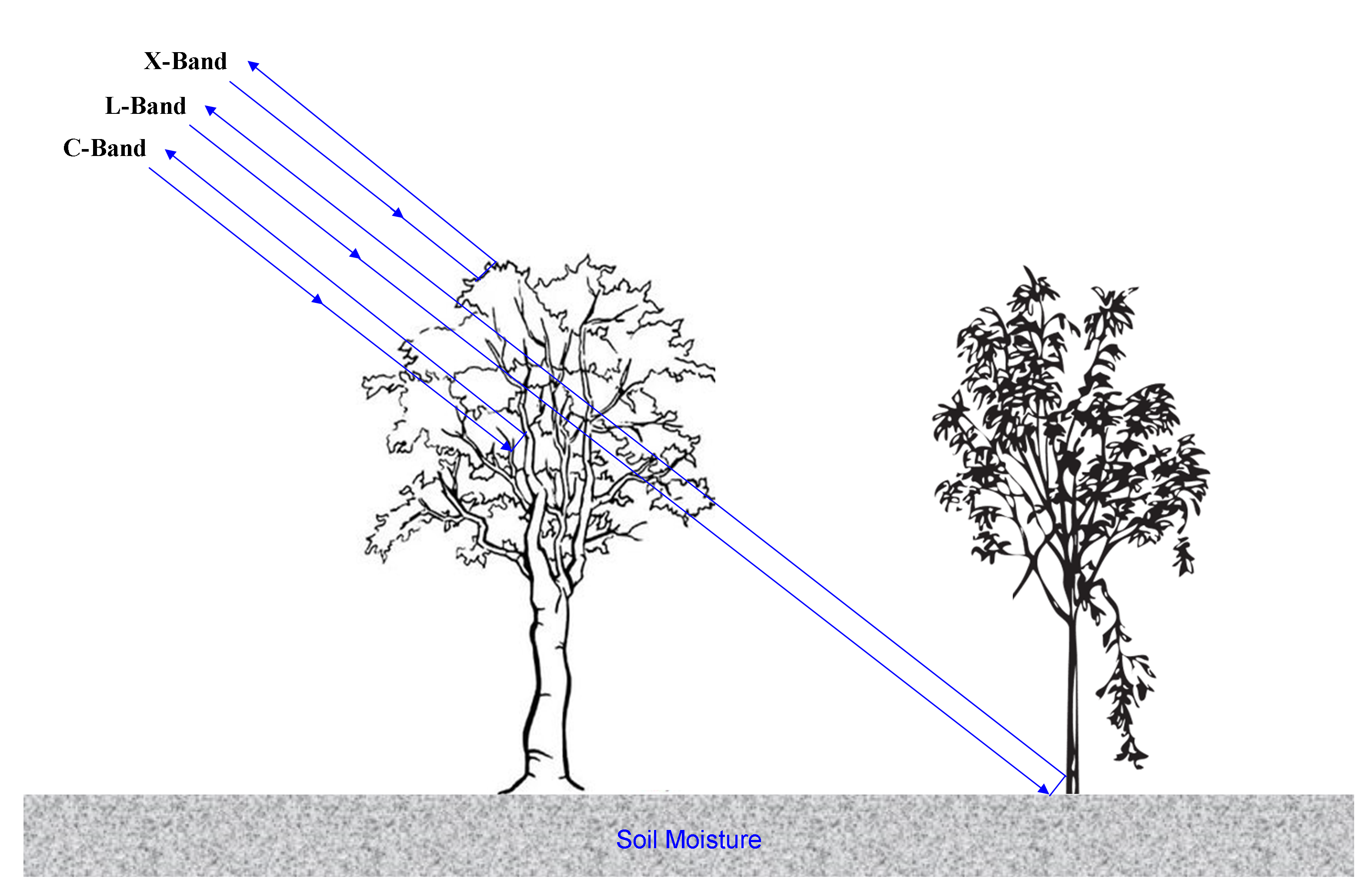
Spatial distribution of SM has been estimated using approach of Mittelbach and Seneviratne (2012) and spatial variance (\(\sigma ^{2} \left( t \right)\))  decomposed into its time-varying and time-invariant contributors using the modified equation (124):

 \(\sigma ^{2} \left( t \right) = \sigma ^{2} \left( \theta \left( n \right) \right) +2cov~ \left( \theta \left( n \right) A_{n,t} \right) + \sigma ^{2} \left( A_{n,t} \right)\)  (124)

where, \(\sigma ^{2} ( \theta ( n))\) is the variance of the temporal mean, \(cov~ \left( \theta \left( n \right) A_{n,t} \right)\) is the sum of the covariance between temporal mean and anomalies, and the variance of anomalies is \(\sigma ^{2} \left( A_{n,t} \right)\). Spatial standard deviation (Rötzer et al. 2015) of SM changes as a power of the extent scale (125) as:

\(\sigma ^{2} \left( t \right) =b*a^{ \mu }\)   (125)

where, \(a\) is the area of the respective extent scale, \(\mu \) is a fractal power and \(b\)  is a parameter.

Patel and Srivastava (2015) have compared SAR derived SM with AMSR-E-derived SM to estimate the bias (126) as:

\(Bias= \mu \left( SAR-derived~SM \right) - \mu \left( AMSR-E-derived~SM \right)\) after Patel and Srivastava (2015)    (126)

Estimated bias is depend on vegetation water content.

8 . CURRENT AND FUTURE DEVELOPMENTS

Space-borne active microwave remote sensing is an efficient technique to acquire knowledge of land surface soil moisture (SM). Several studies have reported comparable results of surface SM using space-borne scatterometer responses to backscattering from soil layer. However, detection and measuring of SM using these techniques require an appropriate filtering of data, site-specific calibration of surface roughness parameters, prior knowledge of the study area, specific research purpose, careful selection of model, different suitable datasets with appropriate time series, etc. Reported success studies are very site-, data- and situation-specific and show uncertainty of models in SM estimations therefore, insufficient to reach global conclusions and applications. Scientific challenge before the community is to develop or modify models and appropriate datasets for SM estimations with simplification and high precision with global applicability for complex bio-physical units. The field is new, active, attractive, challenging and interesting area of research for sustainable land and climate change management.

1. Active microwave sensors perform better than passive microwave sensors for estimations of near-surface SM (Wanders et al., 2012).
2. The Radars, SAR provides high-resolution SM data with poor temporal resolution (Das and Paul, 2015) and more sensitivity to surface roughness and vegetation scattering (Blumberg et al., 2002; Moran et al., 2004; Kurucu et al., 2009; Wang, 2009; Entekhabi et al., 2010). Therefore, needs scientific and technological improvements for operational use (Jeu et al., 2008).
3. PALSAR data has been reported as the most cost effective compared to ASAR versus RADARSAT at \(VV\) polarization (Sanli et al., 2008).
4. Fully polarimetric space-borne SAR sensors, (e.g., ALOSPALSAR, TerraSAR-X and Radarsat-2) with L-, X-, and C-bands are very promising sources for SM estimations (Barrett et al., 2009).
5. Short wavelengths are more sensitivity to soil roughness and vegetation (Paloscia et al., 2010; Blumberg et al., 2002; Das and Paul, 2015).
6. Cross-polarized data is useful for analyzing the contribution of vegetation in the total radar backscattering (Necsoiu et al., 2013). It is suggested for effective applicability of IEM  for SM retrievals (Baghdadi et al., 2006).
7. Co-polarization, \(VV\) channel of ASAR data is more affected by vegetation and less suitable for SM retrievals (Pasolli et al., 2014).
8. More studies should be conducted to include multi-polarization and multi-incidence angle radar configured data over deferent geo-physical conditions before recommendations for operational use (Said et al., 2012).
9. SAR unable to provide suitable datasets with appropriate time series (Barrett et al., 2009).
10. The radar signal are less sensitive to very wet soils (SM > 35 %) and difficult to accurately map of these soils (Verhoest et al., 2008). ASAR data have a limited capability to identify extreme moisture conditions (Pasolli et al., 2014).
11. Backscattering ratio like BR, NBMI are useful for generalizing the relationships between radar backscatter and VSM between 0 and 40%. However, empirical assessments are suggested prior to applications for over large areas (Shoshany et al., 2000).
12. SAR shows promising results of SM retrievals however, they give good results with particular range of incidence angle, to bare soil or grassland areas and can only penetrate the soil surface layer (Bertoldi et al., 2014) therefore, further research with more complex spatially-explicit models has been suggested (Santi et al., 2013).
13. Empirical models are useful to estimate the precise SM within the calibrated conditions (Baghdadi et al., 2006; Wang, 2009) therefore, further studies are recommended for modification in models for wide applicability (Al-Bakri et al., 2014).
14. Empirical models need field measurements for calibration and field measurements are not possible in cases of emergencies (Braun and Hochschild, 2017).
15. Radar backscatters are not only sensitive to soil dielectric constant but also geometric surface of the soil. These relationships have been analyzed in several studies however, the empirical models are very site specific and lack of full understanding of surface geometry for global applicability (Wagner et al., 2007).
16. Theoretical models require surface roughness data and measurements of surface roughness are very time-consuming (Kong and Dorling, 2008).
17. The roughness, vegetation, topography and SM effects on radar response can be separated using multi-frequency or -polarization measurements (Kong and Dorling, 2008).
18. De-polarization models are more sensitive to vegetation cover which disturbing accuracy of the SM (Gherboudj et al., 2011).
19. LAI and RVI are best descriptor to minimize the effect of vegetation on SM retrieval from SAR images using Water Cloud Model (Said et al., 2012; Yue et al., 2016).
20. Calibration based models are very sit-specific and not useful to extrapolate for different bio-physical units (Verhoest et al., 2008).
21. Surface roughness modelling is impractical due to heterogeneity between various fields (Srivastava et al., 2015)
22. Comprehensive assessment needs for analysis of roughness problems to avoid uncertainties of the SM retrievals (Verhoest et al., 2008).
23. The incorporation of topography effect in radar scattering models has been recommended for precise estimations of SM using radar data in hilly regions (Burgin et al., 2016).
24. EM models should be developed and validated for monitoring SM over frozen ground (Necsoiu et al., 2013).
25. Reported causes of uncertainties is SM estimations are incorrect weather forcing, model parameter uncertainty, and incorrect land surface model formulation (Pellarin et al., 2009). Therefore, they fail to provide results with good agreement with experimental observations (Das and Paul, 2015).
26. Results of SM retrieval models vary region to region and can’t be transfer to other regions and require testing different environmental conditions for wide applicability with optimal accuracy (Paloscia et al., 2010; Rötzer et al., 2015).
27. The land surface models are unable to reproduce the rapid dynamics of the near-surface SM at the local and regional scales (Pellarin et al., 2009).
28. Roughness and moisture inversion models are not valid for SM retrievals (Zribi et al., 2002).
29. SAR data acquired in wet season have shown poor relationship with SM (Sano et al., 1998).
30. Simulation of backscattering models depend on roughness description and not satisfactory (Zribi et al., 2002).
31. Linear models require calibration, neglecting roughness and suggested for SM modeling over large area (Zribi et al., 2002).
32. It is difficult to extent the modeling techniques for SM mapping over complex large agricultural area (Srivastava et al., 2015)
33. Well specified research objectives, prior knowledge about the major impact factors and conditions of the study area required for pricise estimations of SM (Barrett et al., 2009).
34. Many scholars have noted need of further research to develop a higher spatio-temporal-resolution for monitoring the surface elements at short-term and small spatial-scales like SM (Liu et al., 2017)
35. Upcoming research should be focused on intensive applications in humanitarian action, robust and automatic analysis with precise and reliable services, short response time for emergency scenarios, improvement in user’s accuracy for human applications, collaboration between scientists and users for minimizing limitations of applications, participation of users will specify their needs, contribute for calibration and validation to improve quality of products (Braun and Hochschild, 2017).

Tables

Figures

Conflict of Interest

Acknowledgements

Abbreviations

References