Keywords

MCDA , Multilayer , Gully Vulnerability Mapping , GIS , Basin characteristics , AHP

1 . INTRODUCTION

Land degradation and erosion have become an ever increasing occurrence as global populations rise and human activities geared towards satisfying social and economic demands. These activities may result in the exposure of land surfaces, thus increasing the vulnerability of land surfaces to water erosion. Water induced soil erosion has been considered as a major cause of loss of land across the global environment (UNCCD, 1994; Valentin et al., 2005; Dreibrodt et al., 2010; Handl, 2012; Ambalam, 2014). Emerging from the soil erosion research in the last few decades, is an attempt to develop different methods and techniques for effective testing and monitoring of soil erosion and gully occurrence (López-Vicente et al., 2013; Lal, 2017; Arabameri et al., 2018).

A gully may be defined as the expulsion of soils on drainage paths as a result of surface runoff. These soils are transported by the means of head ward or by slumping of the drainage banks (Pokhara, 2008; Araki, 2012; Casalí et al., 2015). It occurs as a concentrated movement of water along an eroded channel expunges soils and parent material that may have been too bulky to be destroyed by cultivation practices (Conoscenti et al., 2014; Casalí et al., 2015). Gullies appear as one of the most damaging and complex effects of water erosion. It is known to be the major source of sediment load deposition in a reservoir (Mohsen et al., 2018). In recent times, gully erosion has appeared to be responsible for a substantial loss of properties including; buildings, farm lands and other basic infrastructures (Ajaero et al., 2010). The economic worth of these properties is estimated to be well over a million dollars per annum (Ayele et al., 2015; Goudie, 2018; Medvedeva et al., 2018; Peterson et al., 2018).

Alatorre et al. (2012), Shit et al. (2015), and Wang et al. (2016) have documented some of the major expository environmental factors influencing gully development and dynamics. They are related to precipitation in the form of rainfall, soil, topography, soil moisture, soil erosivity factor, lithology and the prevalent land use land cover (LULC) types in a given area. Rainfall and elevation patterns are the most critical factors that influence surface runoff (Shi, et al., 2017; Xiong, et al., 2019; Pei et al., 2020). Rainfall provides the amount of energy required to transport generated sediments down slope; resulting in lateral and vertical erosion between the generated sediment load with the channel wall and bed. Post et al. (2017), Abdulazeez et al. (2018), Arabameri et al. (2018); Mahmud and Umaru (2018), and Frankl et al. (2019) have reported the effects of gully formation on the environment, LULC, properties and infrastructure, using ground measurements and space-based data. The finding points to a scientific approach for the integration of multiple datasets towards effective management of gully occurrence. In addition, Arabameri et al. (2018) discussed the approaches that can integrate multi-layer information of basin characteristics with high levels of accuracy, in relation to gully expansion and intensity. The stability of a gully depends on the stream erosive process; they include the eroded material from the upstream and any sediment that may grow from the head-cut and channel bottom. Gully occurrences are largely associated with a condition where geomorphic threshold is exceeded due to growth in the inflow of erosive water and sediment erosive capabilities (Huang et al., 2005; Kirkby and Bracken, 2009; Gao et al., 2010; Essien and Okon, 2011; Herzig et al., 2011).

In addition, the nature and distribution of soils and other subsurface materials, the ground steepness, and saturation levels are largely responsible for the circulation of underground hydrology, which provides a suitable drainage controlling factor regime of a location (Kakembo et al., 2009; Daggupati et al., 2013). These conditions are responsible for the regulation of gully morphology amidst the susceptibility of different soil horizons at varied erosive conditions (Conoscenti et al., 2014; Arabameri, et al., 2018). In assessing the contribution of gully occurrence to erosion in a tropical environment, the depth and width characteristics are critical parameters that determine the dynamics of erosion. The interception of a linear infrastructure such as roads and rail lines can form node points where overland flow converges and focuses on the downstream slope (Svoray and Markovitch, 2009; Svoray and Ben‐Said, 2010; Izham et al., 2011; Svoray et al., 2012; Torri and Poesen, 2014; Gudino‐Elizondo et al., 2018).

The heterogeneous attributes of gully instability have necessitated the need for modeling of its dynamism (Maquaire et al., 2003; Sidorchuk et al., 2003; Valentin et al., 2005). Studies that have explored this includes: the empirical models (Jetten et al., 2006; Conoscenti et al., 2014; Pourghasemi et al., 2017), the routine for linear gully erosion models (Kheir et al., 2007; Evans and Lindsay, 2010), and lastly gully morphometric analysis which largely utilizes surface drainage data (Gabet and Bookter, 2008; Jha and Kapat, 2009; Vachtman et al., 2013). The primitive assumption of the later model is based on the insitu based measurements, where different gully inventory data is generated and evaluated for quantification. The morphometric measurements are based on the use of drainage pattern information which utilizes the nature of sediment load characteristics. Drainage based models for gully related studies require quantitative evaluation of water volumes, passing through the drainage and the composition of the transport sediment load which can vary over time (Vaezi et al., 2017; Chang et al., 2018; Caracciolo, 2020). Detailed knowledge of these parameters can effectively reveal a great deal of information, regarding lateral and vertical erosion which influences gully dynamics. Although, these models have provided an effective frontier for the study of gully erosion, the use of empirical data synonymous to models are often grossly inadequate which affects model generalization. Similarly, the use of surface runoff and sediment load characteristics is often difficult to come by and some of the required data points are difficult to access. Evidence-based models still tend to possess uncertainties such as the potential of bias induced weight and the absence of a spatial scope of the area of interest. These uncertainties have the potential of significantly limiting their application, and in addition they justify the application of a geospatial model which will efficiently handle the local limitations, in the absence of model testing and performance. Lucà et al. (2011); Conoscenti et al. (2013); Conoscenti et al. (2014); Dube et al. (2014); Rahmati et al. (2016) and Zabihi et al. (2018) have presented a wide range of techniques including inferential statistics using bivariate data, that can effectively test the reliability of model parameters. In addition, the developed models allow for the regional analysis of gully trends and susceptibility using multilayer information; regarding the different parameters that may influence gully development, management and control. Although, these models were able to overcome the deficiencies associated with the physical model, and were able to provide a technique for quantitatively evaluating the correlation between gully formation parameters and its dynamics using multilayer information, data integration was not effectively provided.

The difficulties associated with the integration of multiple basin characteristics in the assessment of gully vulnerability informed the techniques that allowed for proportional distribution of parameter weight within a given catchment basin. Kavzoglu et al. (2014), Valjarević et al. (2015), Arabameri, et al. (2018), Arabameri et al. (2019), and Vijith and Dodge-Wan (2019) have implemented a GIS-based multi-criteria technique for gully morphometric analysis and assessment by assigning weights to different parameters using the AHP using Saaty (1980) scale. This scale has the advantage of effectively managing the assigned weights to parameters without bias. It determines the consistency ratio (CR) and consistency index (CI) by managing assigned weights through validation. In addition, multiple criteria can be effectively validated with a high degree of reliability and generalization. In terms of model testing, accuracy assessment can be conducted and when applied in modeling, sensitivity analysis can effectively be evaluated to ascertain the level and extent of model reliability. Recent advances in the use of AHP and MCDA based research has focused largely on the management of bias during weight assignment to a parameters. Dashti et al., (2013); Asakereh et al., (2014), Hadji et al., (2017) and Chabok, et al, (2020) employed fuzzy logic in the validation and justification of weight assignment, proving the viability of MCDA and AHP in the evaluation of weights among independent parameters considered to influence the dependent parameter under study.

It is against this background that the research explores the potentiality of remote sensing data, physical data, meteorological and pedological information along with other auxiliary data in modeling gully dynamics in Minna, Niger state. This study seeks to develop a MCDA and AHP technique for the integration of bivariate data sets as an accurate and easy to use in modeling. This will provide a logical rationale for the implementation of sustainable environmental management. The principle of MCDA and AHP provides an effect-based evaluation of all critical parameters that influences the gully instability. In addition, the approach provides a methodology of managing the multiple parameters, by reflecting the magnitude of each in the understanding of gully occurrence.

2 . STUDY AREA

Minna is located on 09º 33ʹ 00" to 9º 45′ 30″ N and 6º 27′ 00″ to 6″ 48′ 15″ E with a total area of 20.44 km² (Figure 1). The study area is circumscribed towards the East by Paida slope extending eastwards in the direction of Maitumbi. The vegetation comprises of open savanna and is very favorable for cultivation. The open savanna is strengthened by the Fadama resulting from the large waterways, alongside intermittent streams laden with thick riparian woodlands. The geography of the study area displays a variation in elevation rising gently from 153 to 436 m above sea level and a steep slopes within the borders East of the study area. The location is characterised by the wet and dry season. During the wet season, precipitation is experienced upto 2003 mm per annum within a period of six months of the average. The dry season is often characterized by an absence of precipitation, fast moving winds with characteristics of dryness and of North Easterlies Origin at the early onset of dryness. Temperature in the study area varies significantly in response to the season. The mean annual temperature is between 28 to 36^ºC. In terms of slope, the study area is dominated mainly by a gentle slopes.

Figure 1. Study area: Minna from Nigeria

3 . MATERIALS AND METHODS

3.1 Criterions

The flow chart (Figure 2) describes the procedure employed in the research data collection and, data sets used and the analysis techniques. Physical parameters in this study refer to: gully inventory data, elevation, rainfall, topography, drainage network data, soil and LULCT as it relates to socio-economic activities.

 

Figure 2. Methodology

 

3.1.1 Morphometric Characteristics

Gully erosion regimes and behavior occur in response to surface runoff, erodability of the surface/sub-surface cover, coupled with several geo-environmental factors associated with its development. The determination of these behavioral attributes along with other geo-environmental conditions is critical to reliability of any gully dynamic modeling analysis. This study therefore, explored the extensive field survey and other conditioning factors to enable the derivation of the criteria for modeling. To this end, gully points were identified using High Resolution Remote Sensing Imagery (HRRSI) of Minna acquired in 2016 with a spatial resolution of 5 m. Using image analysis techniques sequel to correction and ratification, the identified points were based on inference from the spectral characteristics of the features on the image. Total of 186 gully points was identified, out of which a ground trotting exercise was embarked on to identify the validity of the identified gully potential points, as well as generate gully inventory data. A Garmin Handheld Global Positioning System (GPS) was used in tracking and locating the identified points. A measuring tape was also used in determining the gully morphometric data (length, depth and width) after a series of correction of the tape calibration for accuracy. The generated information was coded and developed into a geo data base. Information related to topography was exploited from contour survey maps of Minna, Niger State on a scale of 1:250,000 and a Digital Elevation Model (DEM) of 20 by 20 cell sizes obtained from the Synthetic Aperture Radar, of the Shuttle Radar Topography Mission (SRTM). These were applied in the process of the extraction of slope degrees, elevation, drainage density and distance from infrastructure which were processed and produced into varieties of maps.

3.1.2 Soils

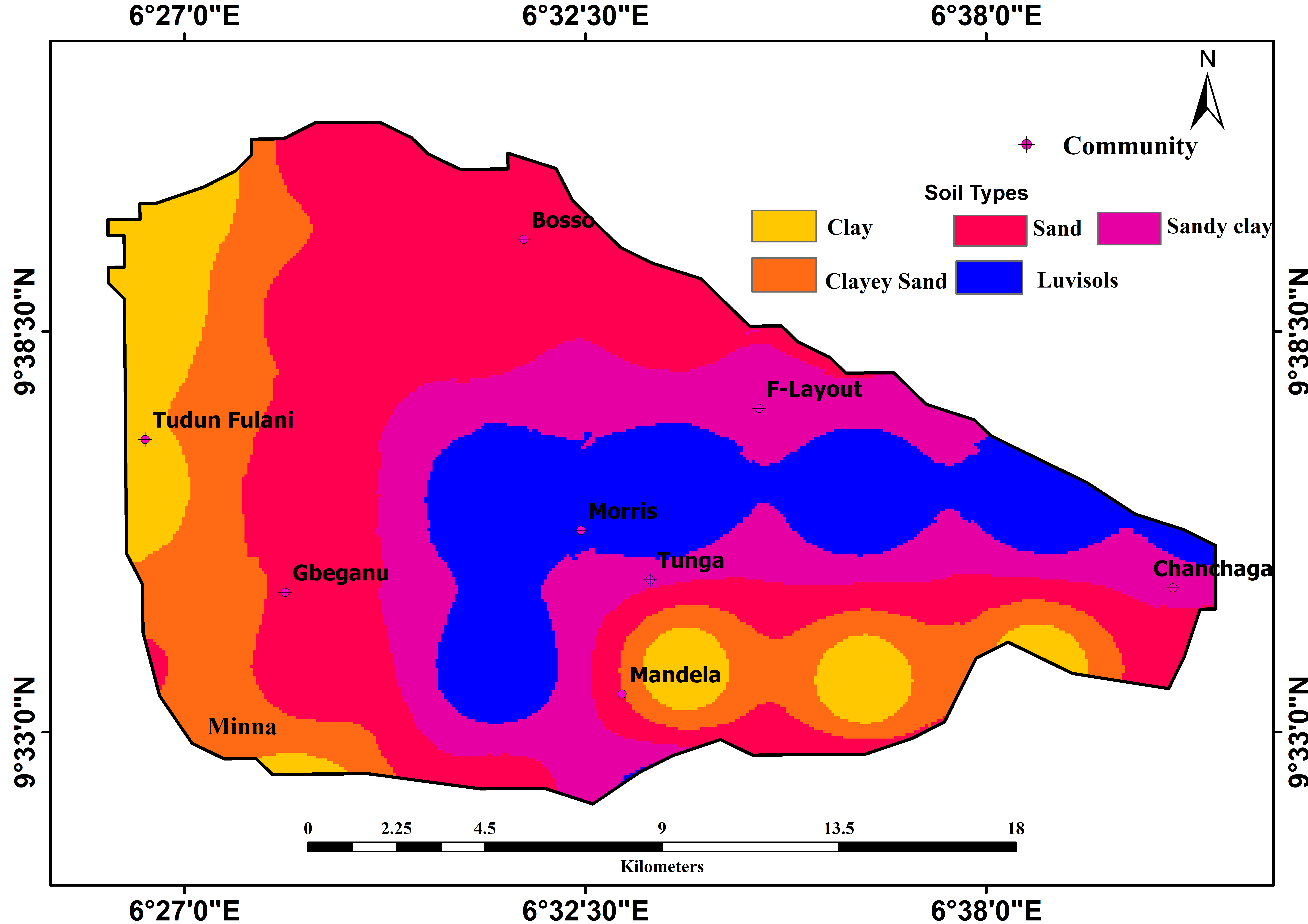
Soil is a critical parameter in the modeling of erosional driven hazards. These properties are associated with the morphological evolution of land features. According to Omid et al. (2016) gullies are dependent on the nature of the prevalent soils and lithology of an area. To explore this further, the soil map of Niger state was collected from the Faculty of Agriculture, Ibrahim Badamasi Babangida University Lapai, Niger State. ArcMap version 10.5 was used to extract the soil map of Minna, Niger State as presented (Figure 3). The processed soil data was validated using other existing pedology data sourced from the State Ministry of Agriculture and Rural Development, along with soil ground control points.

Figure 3(a). Gully length

Figure 3(c). Gully depth

Figure 3(d). Elevation

Figure 3(e). Slope

Figure 3(f). Drainage density

3.1.3 Land Use Land Cover (LULC)

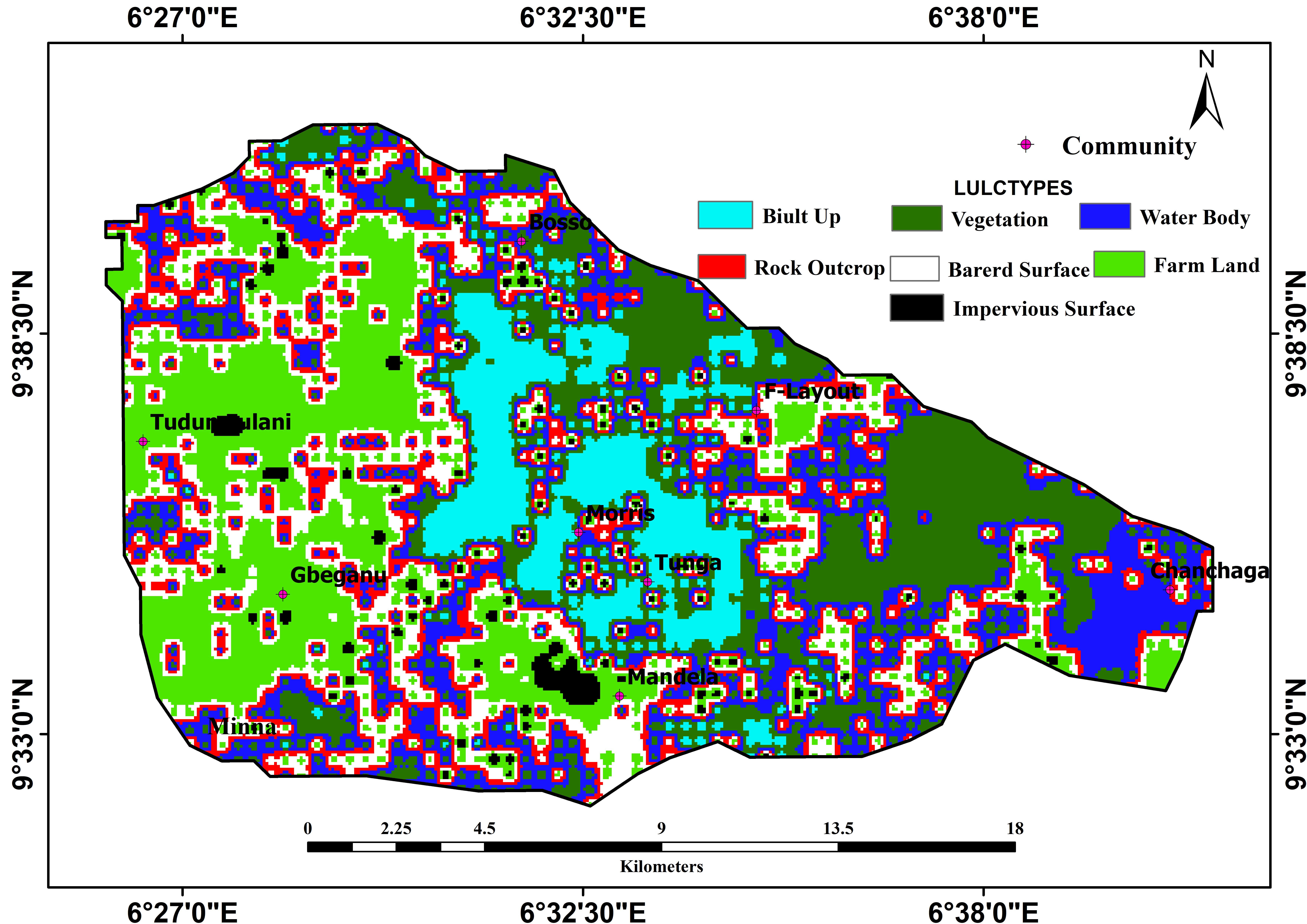
LULC and their management are key components of the hydrological conditioning process of a given location. It is also known to impact on the geomorphological structure instability to gully occurrences (Omid et al., 2016). In general, bare or poorly vegetated surfaces when accompanied by substantial variation in elevation and precipitation are highly vulnerable to erosion. In contrast, densely vegetated surfaces with the same lithological characteristics have vegetation retarding the action of surface flow. This relationship sequence indicates that a negative to low correlation may exist between a densely vegetated surface and erosion, while a positive correlation exists between bared and poorly vegetated surfaces to erosion (Lucà et al., 2011; Sougnez et al., 2011). The acquired satellite data used in this study are presented in Table 1. They are Landsat-7 Enhanced Thematic Mapper Plus (ETM+) and Landsat-8 Operational Land Imager/Thermal Infrared Sensor (OLI)/TIRS images, in C1 level-1. The satellite data was collected for years of 2017 and 2018 in band 7 and 11, respectively.

The processed images were subjected to radiometric and geometric correction to minimize cloud, smoke and dust haze that cause misclassification. The corrected images were then classified using supervised classifications. The result revealed seven (7) major kinds of LULC (Figure 3) in the study area as: built up, vegetation, farmland, water body, outcrop, bare and impervious surfaces. Based on this classification, substantial parts of farm lands tend to be highly gully vulnerable areas, while the built up areas which were the most dominant land use type possessed moderate gully points. Preliminary change detection matrix of the LULC changes is in agreement with the findings of Bashir et al, 2018. They show an increase in urbanization and agricultural land use in the study area; while both activities are found to be encroaching into natural vegetation and some isolated forests.

 

Figure 3(g). LULC

 

Figure 3(h). Soil types

3.1.4 Topography

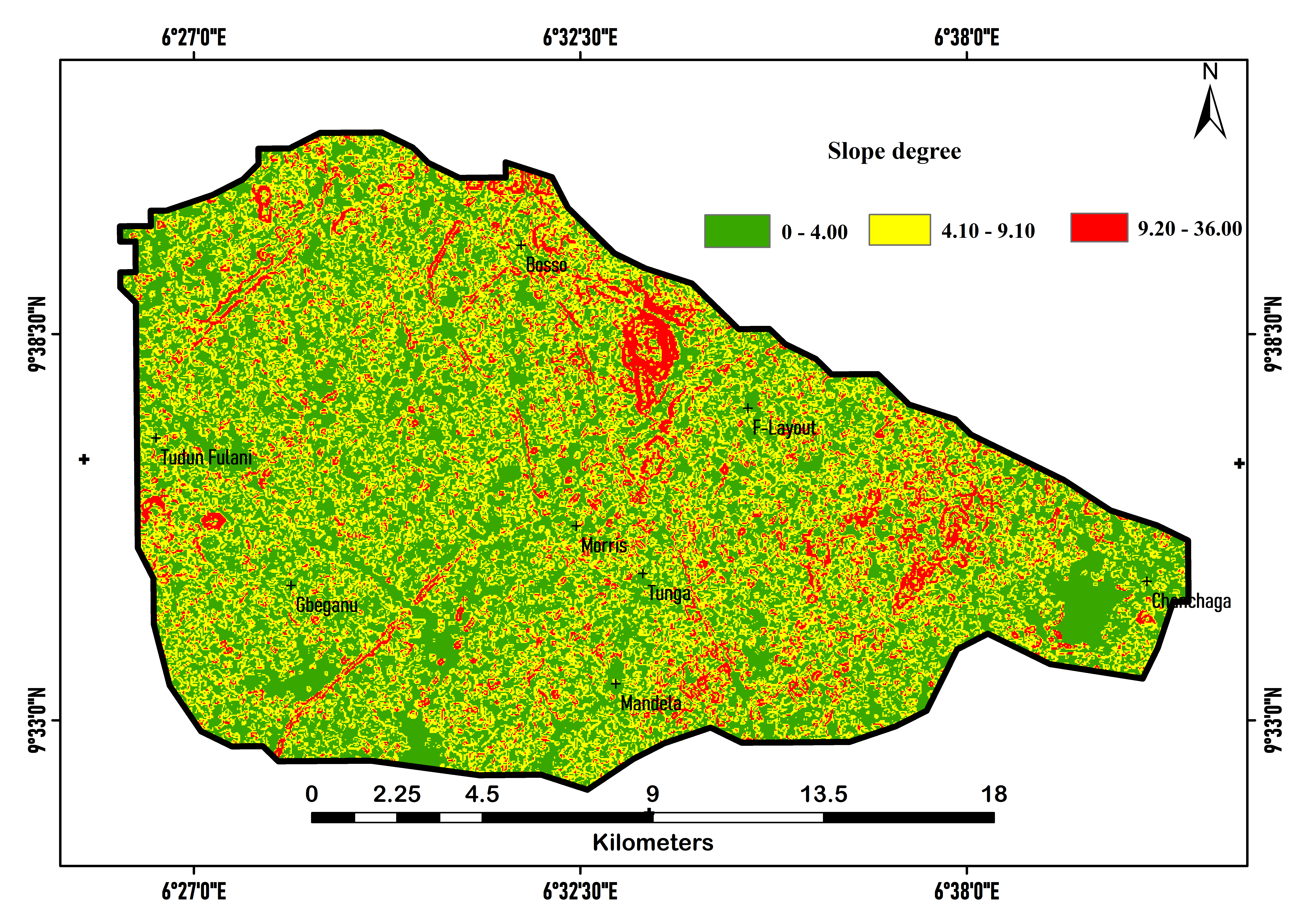
Topographical variables are driving parameters of gully erosion; they enhance the development of fissures; which could be used to envisage gully sidewall instability (Shit et al., 2015). Topographic factors refer to the product of slope length and steepness gradient. Slope refers to the distance from the originating point of overland flow to the point where gradient decline substantially retards erosion and increases deposition (Wischmeier and Smith, 1978). In addition, slope was considered in this study to allow for the inference of soil loss volume from a given length of slope over land of a known elevation. For this analysis, a 10 m Digital Elevation Model (DEM) obtained from the Shuttle Radar Topographic Mission (SRTM) was used to derive slope data. The state ministry of lands and housing provided the topographical map of the study area; and this was used to extract the contour information which has great potential in understanding terrain condition. The derived slope distribution information was reclassified into four classes for weighting and rating based on MCDA and AHP.

 

3.1.5 Drainage System

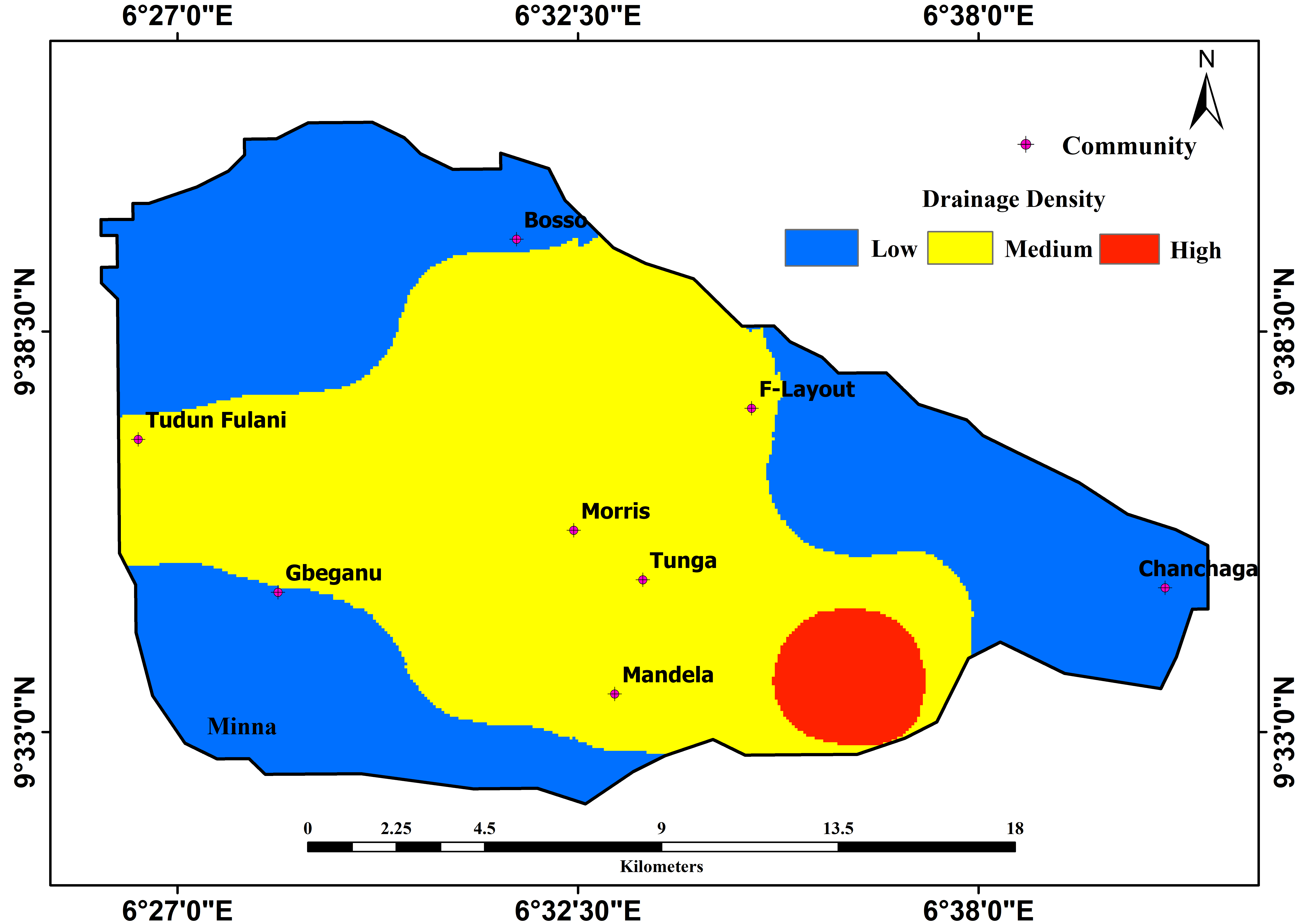
The drainage information used in this study was generated using GIS-based watershed analysis techniques. The study area was delineated and drainage networks were extracted using two major data sets: The DEM and Landsat 7 ETM. The data was subjected to analysis using HEC-GeoHMS tool and the delineated drainages were dissolved into a single data set. A drainage density network analysis was derived from equation 1. Each drainage path was considered and reconditioned into a known cell size within a given grid. The center of the grid approach has the advantage of ease of tracing stream erosion capabilities and thus, enables the linking of erosive power to a cell within the area (Baker et al., 2018; Warren et al., 2019; Garlin et al., 2019). Although the work of Mohsen et al. (2018) indicated the possibilities of using pixels rather than center of a grid in evidential layers, this approach becomes highly degraded due to the inability of the approach to manage slight variation in information flow between two cells. In addition, while the evidential base is capable of managing boundary issues in data flow, the pixel approach makes ambiguous generalizations across all pixels within the area of interest.

Drainage density \(\rho = {∑l\over A}\)                                 (1)

Where,   \(l\)  = total length of stream in (km), and A = cross sectional area (km²)

3.1.6 Universal Soil Loss Equation (USLE)

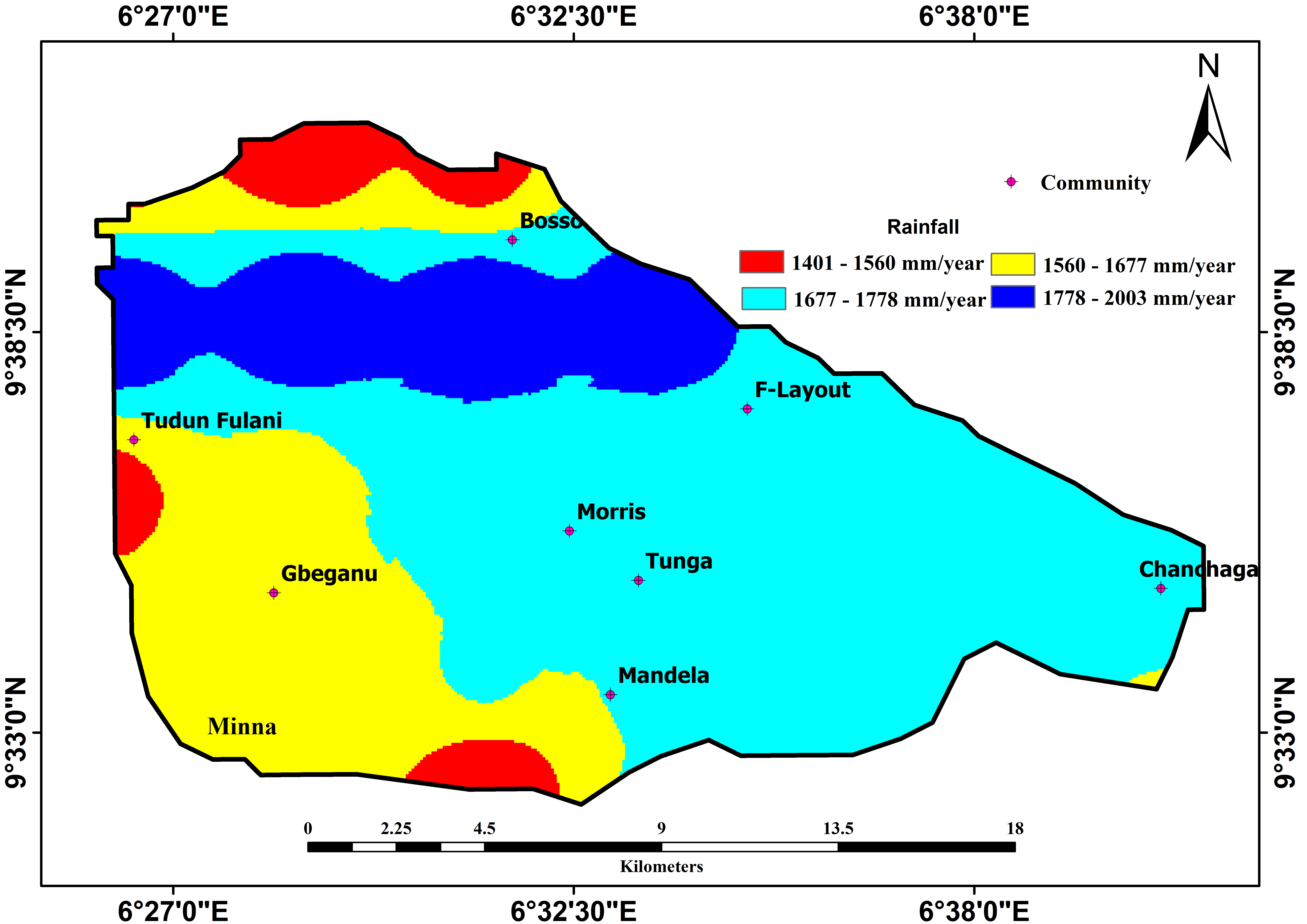
The precipitation data used in this work comprises of rainfall data sets which were obtained from three Nigerian Meteorological Agency (NIMET) stations viz.: Minna airport, Bida and Abuja. Other rainfall data used to supplement the NIMET data were obtained from (1) The Department of Geography, Ibrahim Badamasi Babangida University Lapai weather station. (2) The Agricultural Development Program Observatory Station. (3) The Niger State Ministry of Water Resources Observatory. Furthermore, due to the scanty nature of the obtained rainfall data, remotely sensed data from the National Oceanic and Atmospheric Administration (NOAA) was processed for a 5 year period. The mean annual rainfall for the period under review was then integrated into the grids, which was converted into rainfall density maps using attribute tools in the GIS environment.

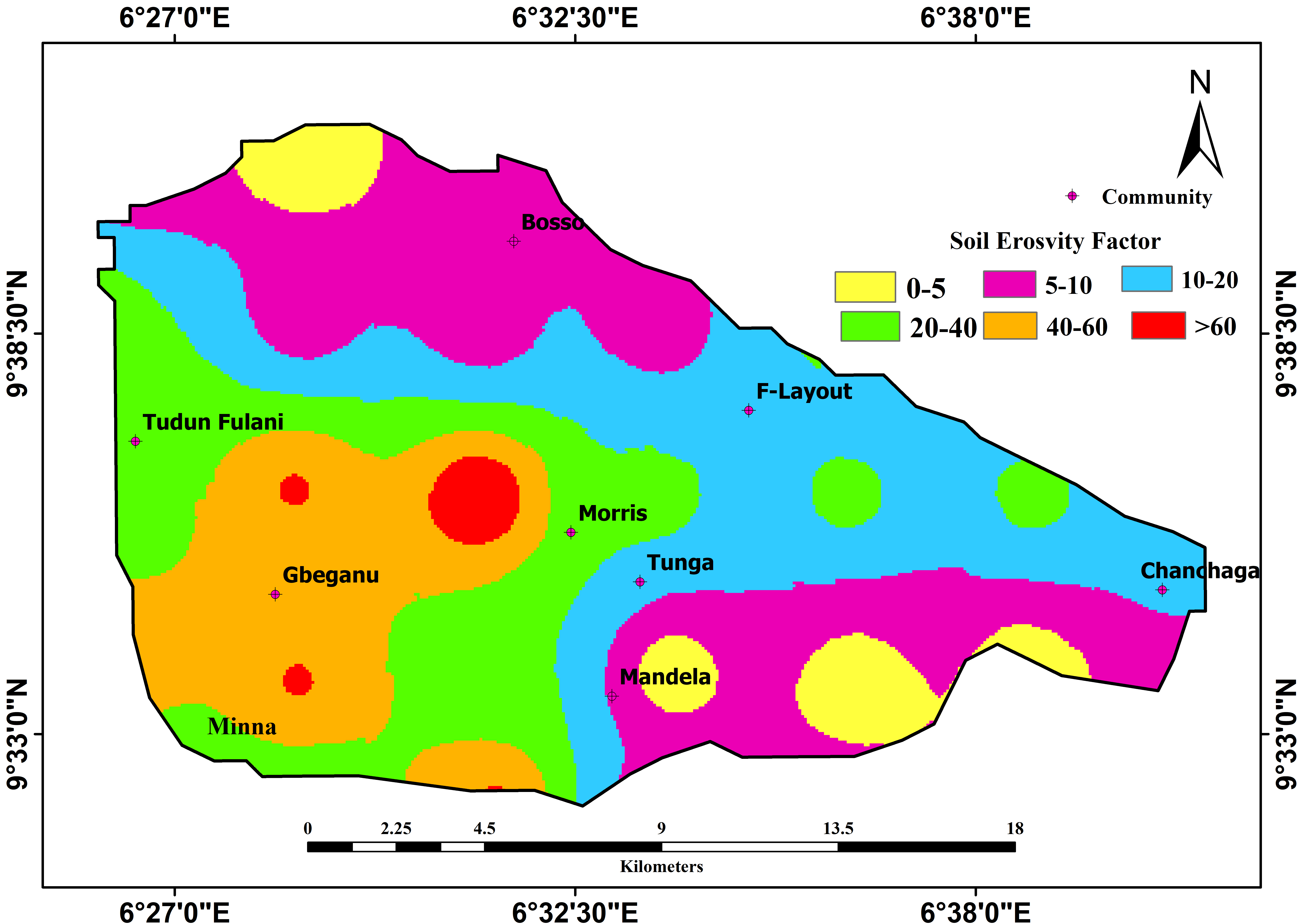
The soil information was used with rainfall data for the estimation of the rainfall erosive factor for the USLE in equation 2 to produce a map of erosive factor in Figure 3.

\(EI_{lx}=(KE×I_x )/100\)        (2)

Where, KE  = Kinetic energy of rainfall is expressed as \(KE=210.3+89 log_I\) , I= Rainfall volume in (cm³), I_x= Maximum volume of the rainfall event and x= Rainfall duration in minutes.

 

Figure 3(i). Rainfall distribution

 

Figure 3(j). Soil erosivity factor

 

Figure 3(k). Slope aspects

 

3.1.7 Topographic Wetness Index (TWI) and Stream Power Index (SPI)

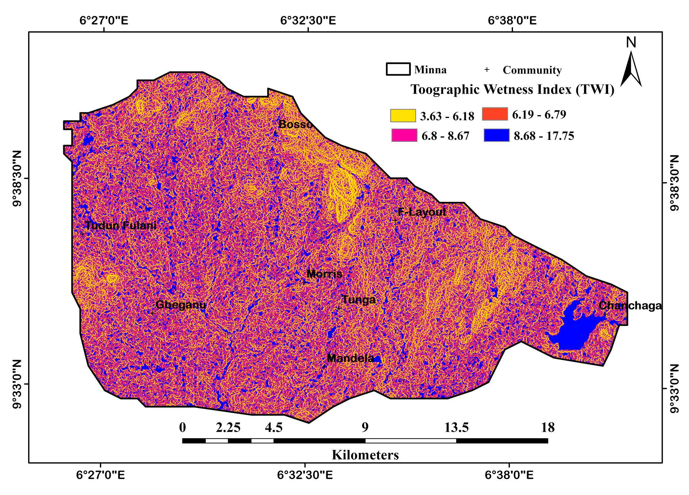
TWI is the spatial distribution showing the zone of saturation and the points of surface runoff generation. Utilization of TWI and SPI provide a viable indicator to understand areas of ephemeral gullies in a watershed. Thus, an area with larger upslope drainage and a shallow slope will produce higher TWI values. This is indicative of a more likely tendency for runoff. TWI value distribution can be used to identify the relative runoff potential zones and catchment (Ågren et al., 2014; Koriche and Rientjes, 2016; Raduła et al., 2018). This model performs optimally when integrated with soil maps to overcome the deficiency of low performance over poorly drained soils (Kakembo et al., 2009; Daggupati et al., 2013). The TWI of the study area was computed using equation 3 and the result generated is presented in Figure 3. The result reveals varying degrees of wetness across the study area with the largest proportion dominated by a wetness index of 6.80 to 17.56. The low index value was prevalent in some isolated elevated areas and among the exposed rock outcrops in the study area indicating low wetness.

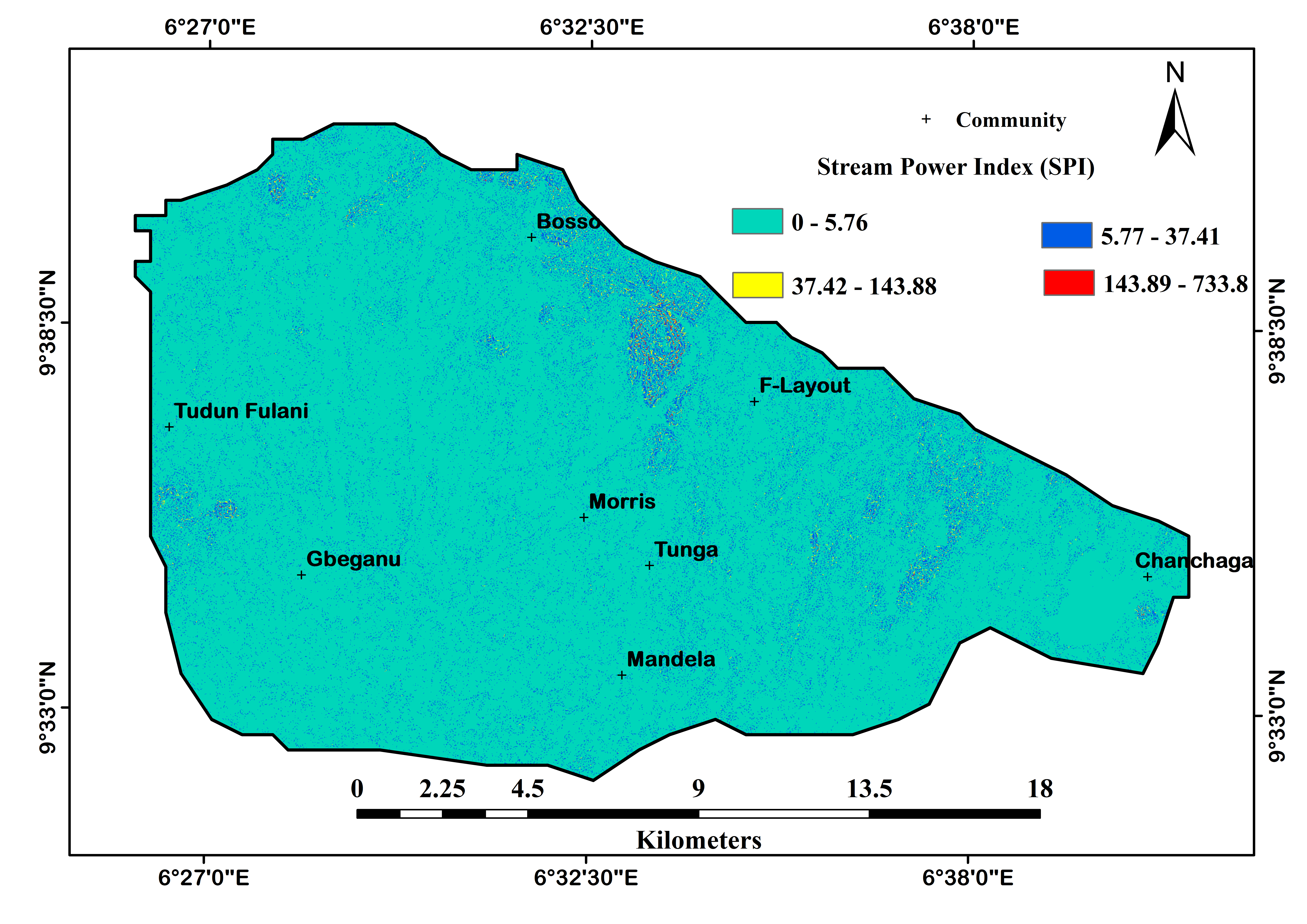
Stream Power Index (SPI) on the other hand, measures the erosive power of a surface runoff based on the hypothesis that the discharge rate is proportionate to the basin. SPI provides an insight regarding net erosion in a catchment basin and the peripheral convexity with net deposition in locations of profile concavity (Pourghasemi et al., 2013). It is the major erosion dominating factor in varying slope areas and a hypothesis for the indication of available potential energy to retain sediments (Dube et al., 2014). This study therefore implemented GIS based determination of SPI using the ASTERDEM (Advanced Space-borne Thermal Emission and Reflection Radiometer Digital Elevation Map) of 30 m as found in equation 4. A cell size of 0.001 and a pixel of 30 were used based on Moore et al. (1991) approach. The result obtained was effectively mapped into different SPI values of the study area as seen shown in Figure 3.

\(TWI = {Inα \over Tanβ+c}\)                                        (3)

where, α= Cumulative upslope drainage area per unit contour length, β= Surface slope or gradient of the area and c = Cell size (0.001).

\(SPI=α×Tanβ\)                    (4)

 

Figure 3(l). Stream power index

 

Figure 3(m). Topographic wetness index

 

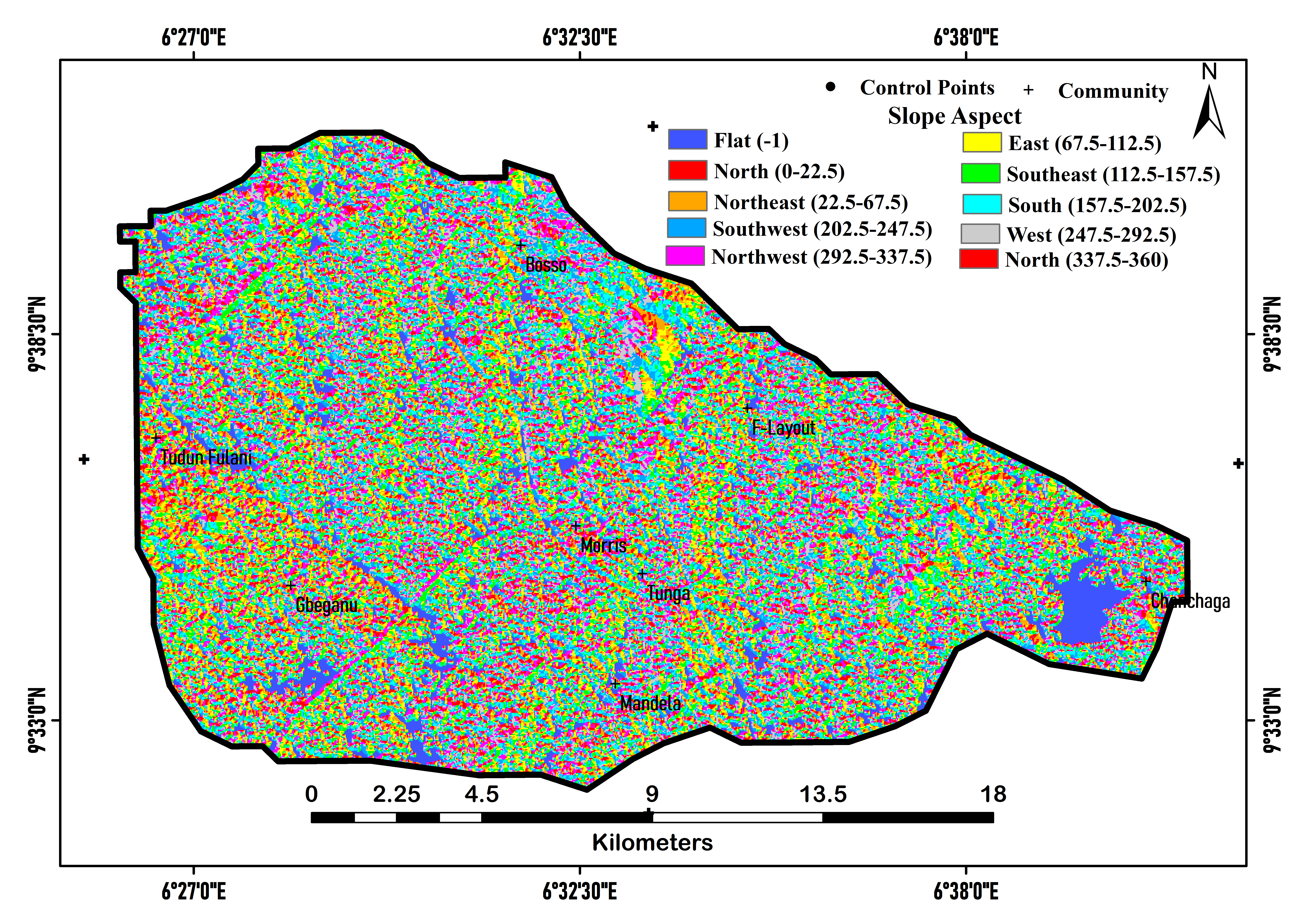
1.1.4 Slope Aspect

The slope aspect map in this study was produced to demonstrate the relationship between gully occurrence and the slope orientation within the study location. Nine (9) thematic layers were derived from the slope aspect as shown in figure 3. About 9 classes correspond to: Flat (-1), North (337.5-360)º, North West (292.5-337.5)º, North East (22.5-67.5)º, South (157.5-202.5)º, South West (202.5-247.5)º, South East (112.5-157.5)º, West (247.5-292.5)º and East (67.5-112.5)º.

3.2 MCDA Weight Determination Using AHP

AHP as developed by Saaty (1980) was used to determine the weight of each factor. The relative weight of the pair wise comparison valued on scales 1-9 is shown in Table 2 and this is used to determine the scores. These scores are assigned based on ranking of contribution to the gully vulnerability index. Due to the subjective nature of criteria weights judgments, there exists a high potentiality of bias resulting in some degree of inconsistency in the assigned weights. Hence, the need for the revalidation of judgments by evaluating the logical consistency of the pair wise comparison matrix (equation 5). Normalized pair wise evaluation matrices of the allotted weights to the specific features were used to derive the Eigen vector as shown in Table 2. Matlab (2010) was used to deduce the Eigen vector values (equation 6) for each of the map themes. The relative importance of the factors under study was shown in the pair wise comparison.

 

\( \begin{bmatrix} 1 & x12 & x13 & \dots & x_{1n} \\[0.3em] \frac{1}{x_{21}} & 1 & \frac{1}{x_{23}} & \dots & x_{2n} \\[0.3em] \frac{1}{x_{31}} & \frac{1}{x_{32}} &1 & \dots & x_{2n} \\[0.3em] \vdots & \vdots & \vdots & \dots & \vdots \\[0.3em] \frac{1}{x_{n1}} & \frac{1}{x_{n2}} & \frac{1}{x_{n3}} & \dots & 1 \\[0.3em] \end{bmatrix} \begin{bmatrix} W_1 \\[0.3em] W_2 \\[0.3em] W_3 \\[0.3em] \vdots \\[0.3em] W_n \\[0.3em] \end{bmatrix}\)

 

and the Eigen value was obtained as follows:

\(λ_{max}= \frac{1}{n} ∑_{(i=1)}^n((∑_{(i=1)}^n \ row \ entry \ of AW)/(i_{th} entry \ of \ row)) \)  (6)

The consistency index (CI) refers to the measure of consistency. This was derived using the equation (7) (Saaty, 1980).

\(CI = {ƛ{max}-n \over n-1}\)           (7)

Where, n= Number of factors, \(ƛ{max}\)  = Eigen value.

Therefore, if the CI value is less than 0.1, the judgments are said to be consistent and there will be no need for re-evaluation. Thus, the result obtained from this step was used since they were consistent.

The consistency ratio (CR) was determined using the relation:

\(CR= {CI \over RI}\)                                  (8)

Where, CI represents the consistency index, RI represents the random consistency index with a value of 0.58, for n = 3 (Saaty, 1980).

Each of the parameters were weighted and scored using the rating 1-6, accordingly. The rating R was assigned and validated using expert vetting according to the order of priority of influence on gully events and dynamics.

 

Table 2. Saaty scale of weight assignment

Less important			Equally important				More important
Extremely	Very strongly	Strongly	Moderately	Equal importance	Moderately	Strongly	Very strongly	Extremely
1/9	1/7	1/5	1/3	1	3	5	7	9

 

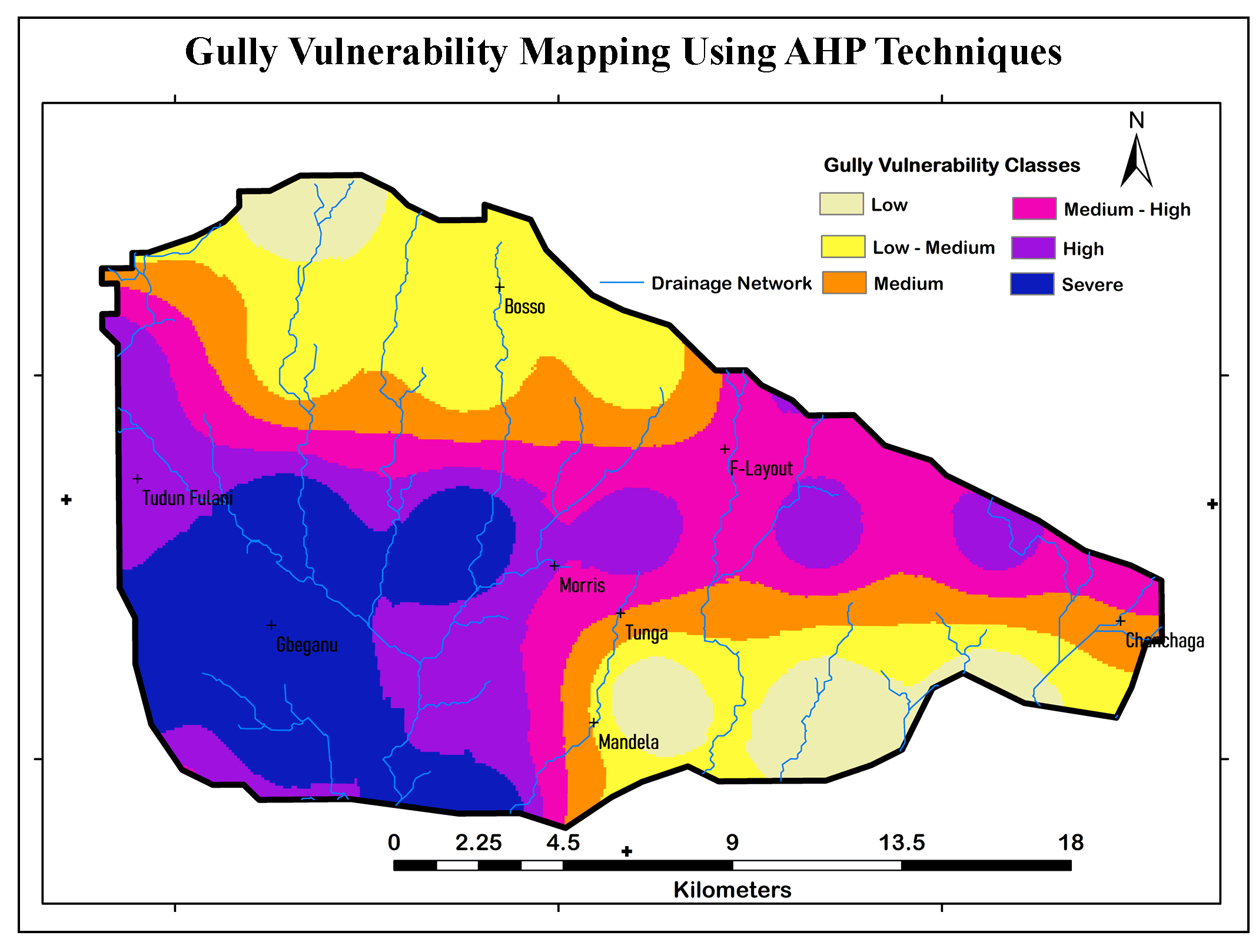
3.3 Estimation of Gully Vulnerability Index

The final map was developed using:

\(GVI=∑W_i R_i \)         (9)

Where, W_i refers to the weight of the gully in parameter i and R_i refers to the score rating of parameter i.

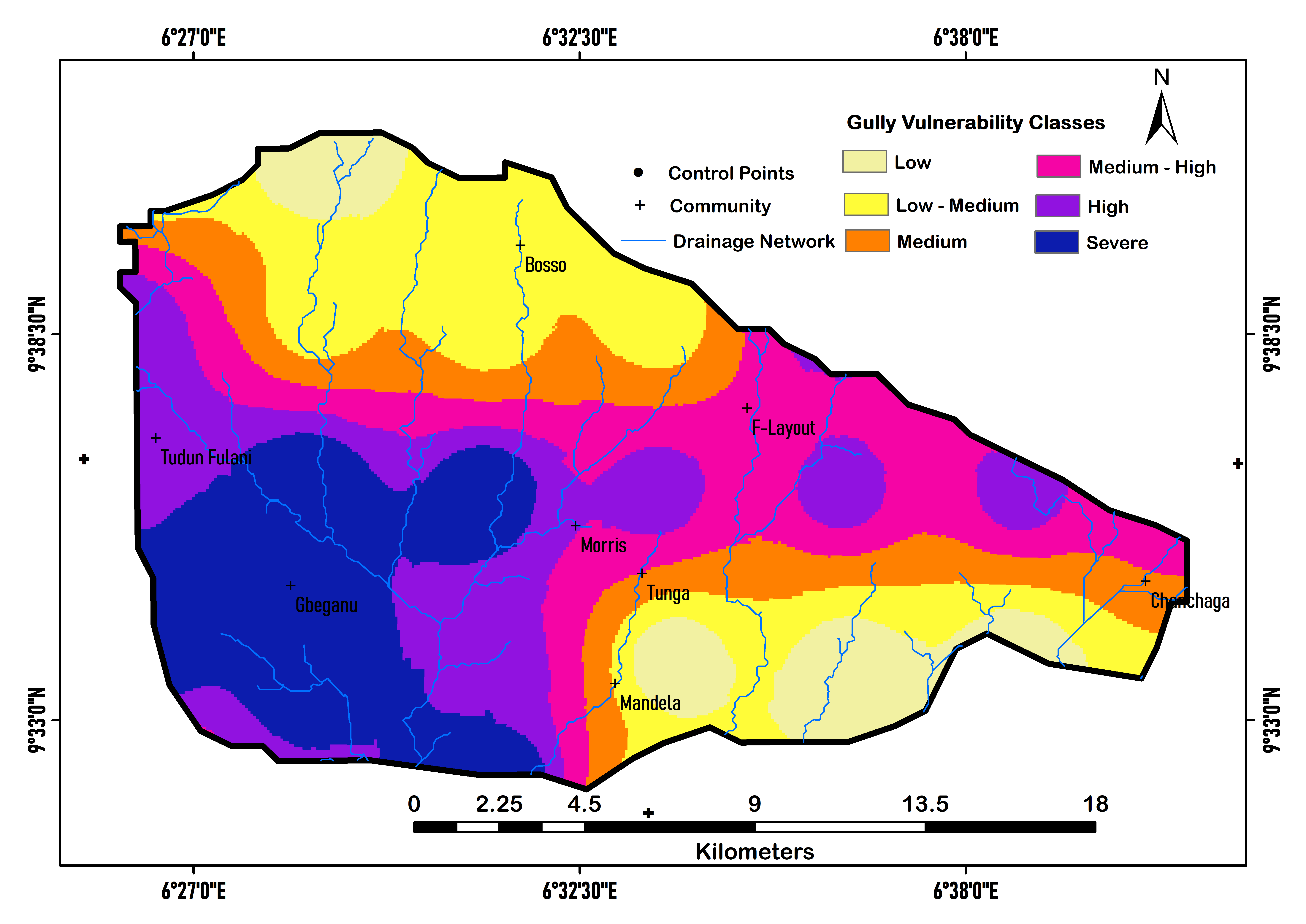
The estimation of the Gully Vulnerability Index (GVI) was developed using a weighted linear combination in equation 9. The normalized weighting of each of the selected criteria and the potentiality parameters relative to each of the selected criteria, was then calculated to obtain the total weights of the different factors (Figure 3) using weighted linear combination approach in equation 10 and presented in Table 3.

\(GV=E_{NW} E_i+S_NW S_i +RF_{NW} RF_i+SL_{NW} SL_i+LULC_{NW} LULC_i+DD_{NW} DD_i+GC_{NW} GC_I+SA_{NW} SA_i+SPI_{NW} SPI_i+EF_{NW} EF_i +TWI_{NW} TWI_i\) (10)

where, GV is Gully Vulnerability, E is Elevation, S is soil, RF is Rainfall, SL is slope, LULCT is the Land Use Land Cover Type, DD is the Drainage Density, GC is the Gully Characteristics, SA is the Slope Aspect, SPI is the Stream Power Index, EF is the Erosivity Factor, TWI is the Topographic Wetness Index, NW is the Normalized Weight and i is the weight of individual factor.

 

Table 3. Criterions and weights

Criterions	Sub-criterions	PIGOD	Rating	NW (%)
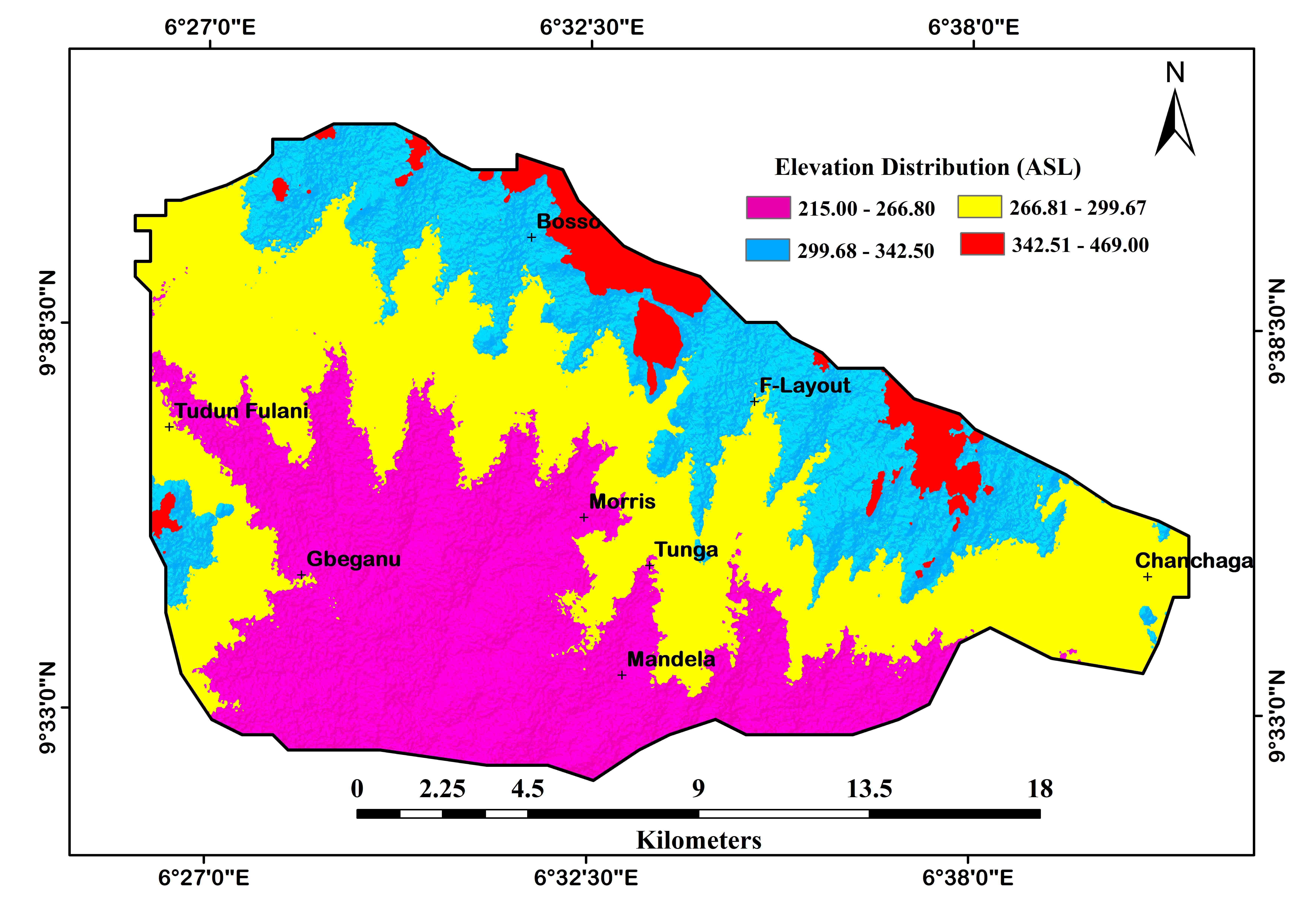
Elevation (MSL)	215.00-266.80	Low	1	7.16
	266.81-299.67	Medium	2
	299.68-342.50	Medium-High	3
	342.51-469.00	High	4
Soil	Clay	Very low	1	10.12
	Clayey Sand	Low	1
	Sand	High	4
	Sandy clay	Medium	5
	Luvisols	High	6
Rainfall (mm)	1401-1560	Low-Medium	1	8.30
	1560-1677	Medium	2
	1677-1778	Medium-High	3
	1778-2003	High	4
Slope (Degree)	0.00-04.00	Relatively flat (Very high)	5	8.56
	4.10-9.10	Gentle slope (low)	1
	9.20-36.00	High slope (medium)	1
LULCT	Built-up	Low	4	10.12
	Bared surface	Medium	5
	Farm land	Medium to high	6
	Rocky outcrop	Very low	1
	Vegetation	Low	2
	Water body	Low to Medium	3
Drainage Density	Low	Moderate	3	9.31
	Medium	Medium-High	2
	High	High	5
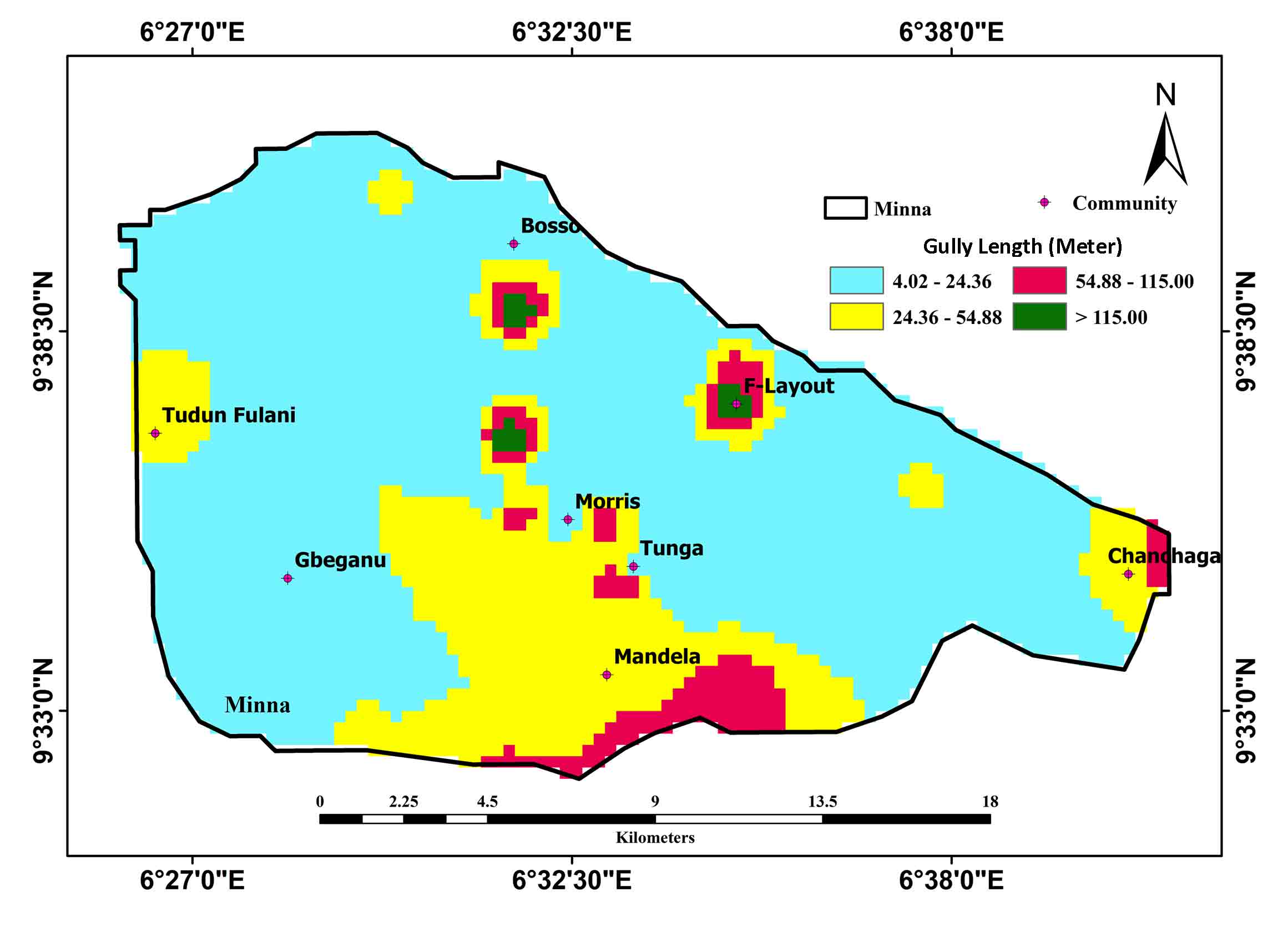
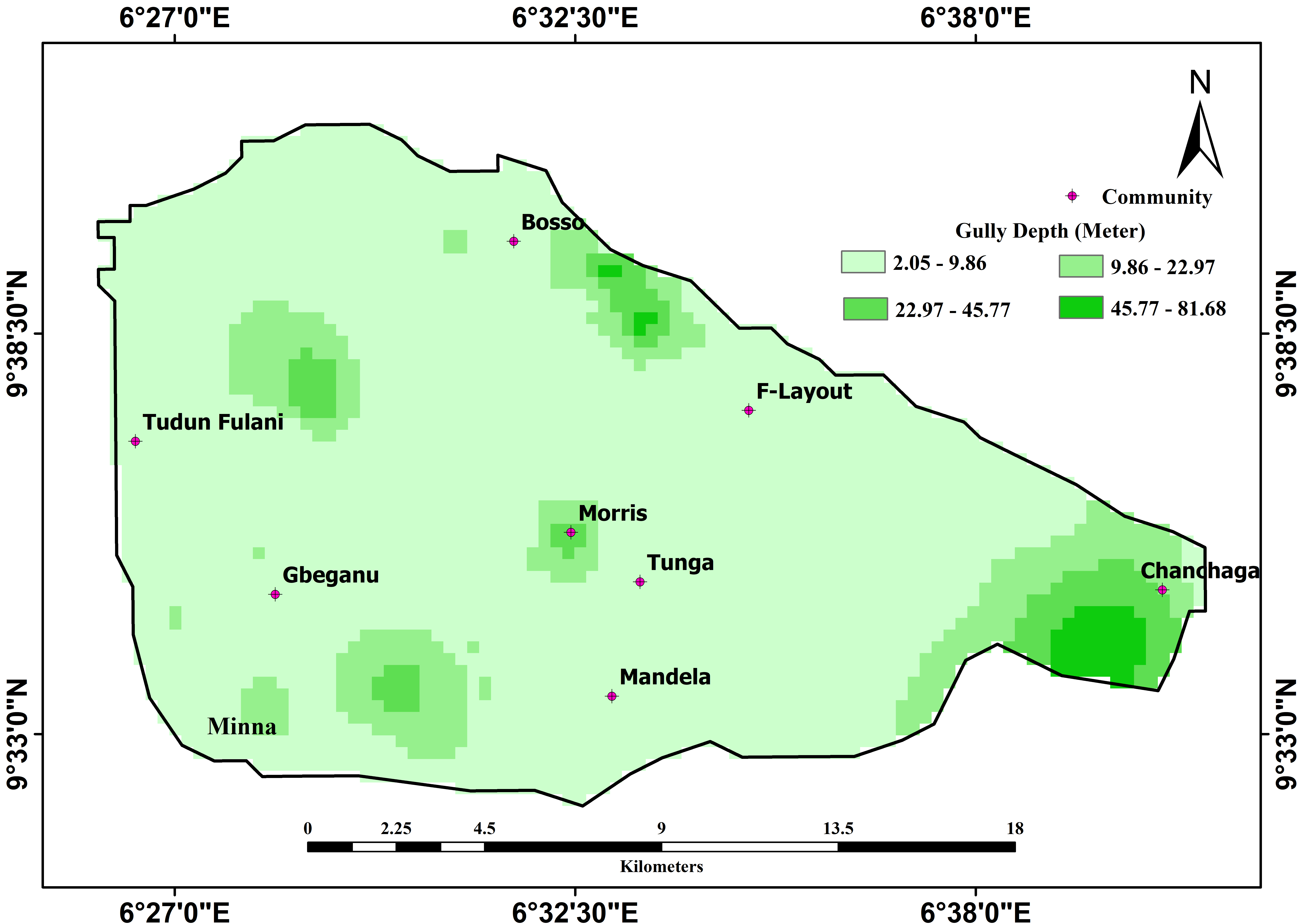
Gully Morphology (m)	Length	Medium	2	9.86
	Width	Medium - High	3
	Depth	High	4
Stream Power Index	0-5.78	Low	1	5.62
	5.79-37.42	Medium	3
	37.42-143.88	Medium-High	2
	143.88-733.80	High	4
Topographic Wetness Index	3.63-6.18	Low	1	6.01
	6.18-6.79	Low-Medium	2
	6.79-8.67	Medium-High	3
	8.67-17.76	High	4
Soil Erosivity Factor	0-5	Slight	1	7.79
	5-10	Moderate	2
	10-20	High	3
	20-40	Very high	4
	40-60	Severe	5
	>60	Very severe	6
Slope Aspect (degrees)	Flat	Negligible	1	3.15
	Northeast	Low	2
	Southeast	Low	2
	Southwest	Low	2
	Northwest	Medium	3
	North	High	4
	South	Low	2
	West	Low	2
	East	Medium	3

 

4 . RESULTS AND DISCUSSIONS

4.1 Criteria Conditioning

The gully dynamic factors and criteria rating of different classes show the importance of the different classes of the eleven factors. It can be observed from Table 3, that the minimum elevation has a value of 215 m from ASL with the lowest weight of 1. The maximum elevation distribution in the study area was 469 m with the highest weight of 4. Inference from these ratings indicates a strong positive correlation between elevation values and surface erosion. This phenomenon when related to gully occurrence will increase as a result of an increment in elevation and decline in response to a reduction in elevation. The nature of sub-surface lithology/soil is critical to the formation of gully conditions which is often initiated by sheet erosion. The presence of luvisols is a major lithology that is highly susceptible to gully occurrences. Thus, luvisols soil type was scored the highest weight of 6 and sandy clay had a score weight of 4. The most stable soil type that is least susceptible to gully occurrence is clay. Clayey soils have tighter pore spaces that make them resistant to lateral collapse and they are redundant to corrosion, due to movement of lateral particles. Artificially, natural mineral can be combined with organic substances for soil stabilization and enhanced physical and mechanical properties (Gholamiderami et al., 2020). Precipitation inform of rainfall is a major factor and the most active agent of soil erosion in the tropical region (Mancino et al., 2016; Gaubi et al., 2017). It becomes more active when accompanied by highly unstable soil and rapidly changing elevation. Soil types are key determinants of gully conditioning; as they provide erosive surfaces and topographic wetness factors which are necessary for lateral erosion. Slope classes of 9.20-36.00 degrees have the highest weight of 5 and the lowest value of 1. Slope values of 9.20 to 36 degrees, indicate that an increase in slope gradient to a certain value will increase the chances of gully occurrence; and upon reaching a peak value, decreases. The gully points in the study area appear as a linear feature adjoining many of the drainages, except for some few isolated cases around the developed or built-up areas. The gully morphometric parameter of the highest weight (5) is the width. A gully width is likely to expand rapidly thus, destroying any structure along its path and result in increased damage. The capability of LU types in influencing the erosion process is more significant on bare and sparsely vegetated surfaces thus, experiencing rapid erosion, as compared to densely vegetated areas with reduced infiltration and low erosion occurrences (Lucà et al., 2011). Farmland in LULCT was scored 6 and indicative of the maximum weight of criteria in this group. Farmlands are often associated with most favorable conditions of soil degradation due to the destruction of soil particles which make it more vulnerable to erosion.

A high-density (length per unit square area) class was weighted as score 5; marking the highest amongst weights in this category. Higher drainage densities were linked with more vulnerability to gully erosion due to the creation of a favorable wetness necessary for the formation of underground drainages, and the provision of strong erosive (both lateral and horizontal) capability of the adjourning contributions. In SPI, the highest weight of 4 was assigned to the maximum index of 143.88-733.80, representing a peak region of runoff into drainages. The SPI of drainage indicates it erosive power, this is a requisite condition for the formation of gullies especially in a high slope degree with poor soil structure and precipitation. It is expected that the higher the SPI, the more rapid the gully formation will be, especially when the gullies are adjunct to drainages as evident in the study area. In the study area, a TWI of class >8.67 has the highest score of 4, demonstrating a greater likelihood of gully incidence within the study area. In general, a higher TWI is an indication of a higher infiltration rate (Mousavi et al., 2017). This also has potential of facilitating the formation of piping and roof collapse (Mohsen et al., 2018) as a result of a close depression, sink holes, blind gullies. In the TWI scenario, the relationship between gully occurrence, and slopes of >36 degrees, soil and SPI of >140 largely reflect a strong positive magnitude of susceptibility in the study area. In addition, an elevation along with the TWI at a reliable class can also create an enabling environment for a rapid expansion in gully width, especially when these gullies are adjunct to an existing network of streams. In this study, the classes of Soil Erosive Power (SEP) varies from slightly above 0 to a class of 60. The highest criteria weight of sixty indicates a high potentiality of gully widening as the SEP value increases. Lucà et al. (2011); Ganasri and Ramesh (2016) and Gaubi et al. (2017) observed a similar relationship between the severity of a gully occurrence in length, width and depth as SEP increases. Usually, the intensity of gully destruction is largely due to its ability to widen as a result of wind and other forms of erosion such as sheet and rill. Their development may create a sub-surface gully which might sprout up to the surface; consequent to the creation of a large void below the structure or along its path especially in karst regions. Slope aspect is a description of slope inclination orientation. It influences rainfalls, wind Coriolis effects and surface exposure to agents of denudation (Yalcin and Bulut, 2007; and Wang et al., 2015). The slope aspects of the North and North-West were rated as 4 and 3, while the remainder were rated 2; with an exception one which was considered negligible and rated 1. In the study area, the nature of the surfaces along with the soil and climatologically variables make it suitable for the dominance of North and North West; as the slope aspect with the highest erosive power.

4.2 Gully Vulnerability Mapping

The implemented method provides us with a technique to generate a gully susceptibility rate on a spatial scale in Minna, Niger State Nigeria. The intricate relationship among gully influencing factors and environmental attributes were adequately accessed using the MCDA and AHP technique by evaluating the different criteria. The consistency ratio and the gully vulnerability index were used to validate the inferential weights assigned to different maps. The spatial distribution of gullies was produced using a substantial number of input variables. For enhanced visual interpretation of the classified gully vulnerability classes, the data was reclassified into a unique thematic map layer using ARCGIS 10.5. Each of the thematic layers was grouped into a class of six representing low, low-medium, medium, medium-high, high and severe vulnerability as depicted in Figure 4.

The low and low to medium vulnerability areas extends from Bosso community to some parts of Gbeganu area of Minna. This region is mostly confined to developed areas. These areas are often characterized by low vegetation, poor water infiltration and low soil erosive factor due to the predominance of impervious surfaces which according to Patil (2018) it significantly retard soil degradation. In addition, the prevalence of clay and clayey sandy soil is most likely to be responsible for the low gully events in the area, due to tighter pore spaces between soil particles which can influence permeability and the subsequent erosion potential of an area (Marot et al., 2016 and Sajedi‐Hosseini et al., 2018). The major gully driving factor of the medium vulnerability zone is the nature of the soil which has direct correlation with the soil erosivity factor and slope (Conoscenti et al., 2014 and Zabihi et al., 2019). This result is in conformity with the soil, rainfall and erosion relationship documented in the work of Kirkby and Bracken, 2009; Conoscenti et al., 2014; Aminu and Jaiyeoba, 2016 and Teng et al., 2016. Slope orientation, soil and land surface conditions are intricate but interrelated factors influencing gully development especially in the context of lateral erosion and energy required to transport the generated sediment load along the gully path. The amount and rate of erosion is inversely proportional to gravity which is driven by slope. A higher slope value accompanied by luvisols is highly vulnerable to erosion due to the low particle cohesion. Slopes provide the maximum gravitational force required to transport sediment load either in suspension or solution along the gully banks by changing from potential energy to kinetic energy.

Medium to high gully vulnerability regions majorly correspond with locations that are well-planned layouts characterized by either poor drainage design or complete absence of drainages. The poor drainage condition accompanied by poor soil particle cohesion provides suitable surfaces for maximum erosion since runoff from buildings are not properly coordinated and controlled along in a designed channel for urban storm water management (Izham et al., 2011). Further, examination of LULCT by this study, revealed dominance of farmland and some isolated cases of built-up areas especially behind army barracks Minna and Mandela compared to the city center. The destruction of the soil structure and texture associated with the clearing of vegetation cover, and poor agrarian practices (Souchere et al., 2003 and Gordon et al., 2008), might have create a conducive condition for the development of gully erosion which often begins in form of sheet or rill erosion; and finally captures the available drainage network in the area. In addition, the constant exposure of the soil to the direct impact of rainfall can further exacerbate the process of soil erosion. The process of erosion and transportation will further result in the widening of gullies, when the floor of the created gully canal collapses. The dominance of lateral erosion and poor soil particle cohesion is largely responsible for the expansion of the gully depth and creating instability in its dynamics.

4.3 Gully Distribution and Vulnerability

The spatial analysis of the output performed in this study, shows a varying magnitude of vulnerability of gullies across the study area as presented in Table 4. The result shows 8.67% of the study area showing low vulnerability, low to medium vulnerability (21.25%), medium vulnerability (13.68%), and medium to high vulnerability (19.47%), high vulnerability (18.06%), and severe vulnerability (18.88%), respectively. The overall analysis shows the dominance of low-medium gully vulnerability area of up to 21.25%%. The result of this study by implication, suggests that a substantial level of gully erosion covers the study area, which if not checked might hamper infrastructural development and human settlement in the study area. The narrow margin between the high and severe vulnerability of 18.06% and 18.88% is a clear indication of a similarity in gully occurrence conditions. This condition might have arisen from the homogeneity in precipitation which provides a similar surface runoff denudation across the similar soil formations.

Figure 4. Gully vulnerability

4.4 Predictive Accuracy and Performance of the Model

In this study, a visual predictive check approach was employed in assessing the accuracy of the developed model’s predictive capability. To this end, a total of 60 training samples representing 33% of 180 points were selected for validation. The results obtained are presented in Table 3. The result shows that out of the total of 13 control points where training samples were selected, only three (3) representing 15.38% failed to compared to the obtained model vulnerability prediction results. In addition, ten (10) representing 84.62% were consistent with the map prediction. The high success rate of the predictive capability of the model is an indication of the excellent capability of the developed model in assessing the gully vulnerability in the study area. The accuracy of 84.62% of the predictive capability of the model revealed that GIS-Based MCDA and AHP has an excellent performance value and thus, suitable for gully erosion vulnerability mapping. Further statistical evaluation of the model performance accuracy (Table 4) from a regression plot graph (Figure 5), shows a high R-square value indicating that, the predicted map and training sample used in developing the model are well fitted. This further indicates that the employed MCDA and AHP demonstrate a high efficacy in gully prediction by integrating a multilayer data set.

Figure 5. Ground checked and modeled vulnerability

5 . CONCLUSIONS

This study adds to the academic literature which supports the validity of employing the MCDA and AHP approaches in the understanding of gully occurrence and vulnerability. It further demonstrates the efficacy of evaluating multiple criteria influences (by assigning weights based on ranked importance) on gully development The findings show an accuracy of 96% (Figure 5), thereby demonstrating the viability of this approach in the integration of physical, lithological and precipitation data, along with drainage characteristics in the understanding of gully vulnerability classes. Even though the low to medium gully vulnerability class (21.25%) was dominant in the study area, it is also important to note that the severe vulnerability gully class covers a substantial area of 18.88%. This has affected the buffer zones in the study area and could create risks to urban growth.

The integration of the MCDA and the AHP into GIS workflow provides an effective approach critical to minimizing the limitations associated with gully occurrence analysis, using a singular basin characteristic; as evidenced in the existing erosion studies. The findings of this study provide an effective model for estimating gully vulnerability; which is critical to the understanding of soil erosion. The results obtained will be equally important to the fields of civil/water engineering, urban planning and government agencies such as the environmental protection agency. This will be pertinent in determining gully risk zones, circumspect urban development, tracking and proper infrastructure construction plans for long-term gully disaster mitigation. The methods and techniques employed in this study can be applied in regions with similar physical, lithology, climate and hydrogeological conditions.

6 . FUNDING AGENCY

This research is funded by Tertiary Education Trust Fund (TET Fund) as Institutional Based Research Grant (IBR) 2017.

Tables

Figures

Conflict of Interest

Acknowledgements

Abbreviations

References