Three tube wells were sampled and positioned along each transect at regular intervals making a total of 18 wells.
The ultimate aim of the study is to establish relationship between groundwater yield and river flow.
2-way ANOVA at 5% level of significance showed no significant difference in the groundwater yield.
Average yield of wells for evening hours recorded a higher yield of 3.3 L/s (55.93%).
The study can be replicated in other sedimentary formation areas to validate.
Abstract
This paper proposed a model explaining variation of shallow groundwater yield and dynamic level with respect to river location in the floodplain of Hadejia, along Hadejia River Basin of Jigawa State, Northwestern Nigeria. To achieve the aim, six transects were established within one km2 of floodplain and were oriented perpendicular to the river channel. Three tube wells were sampled and positioned along each transect at regular intervals making a total of 18 wells. Pumping test, which was repeated four times at 15 minutes interval in both morning and evening hours was used to measure groundwater yield. Multivariate statistical tools such as analysis of variance, Pearson product moment correlation, and cluster analysis were used, respectively, to test the research hypothesis and to classify sampling points into similar groups based on groundwater yield. Results show that the average yield of wells for evening hours recorded a higher yield of 3.3 L/s (55.93%) than the yield in the morning hours of 2.6 L/s (44.07%). Further, the 2-way ANOVA at 5% level of significance showed no significant difference in the groundwater yield related to relative location of wells in morning (p value, 0.30>0.05) and evening (p value, 0.21>0.05) hours. The results of ANOVA revealed no statistically significant difference between the points. It suggests that the adopted model can be applied in other similar sedimentary basins with a view to validating it. A decision support system is recommended among the strategies to improve groundwater resources management in the area.
Water is one of the environmental resources that make life possible as well as providing the quality of life (Patel et al., 2016). Water is used for a number of diversified human activities, principally the drinking and agricultural use (Olofin, 2011 and 2016). For this reason and other vital importance, water has been captured in the agenda, 1, 2, 3 of the Sustainable Development Goals (MDG, 2006). Reliance on groundwater for daily usage accounts for the one third of world population (Kura et al., 2016; Shin et al., 2020). Surface water scarcity resulting from poor rainfall regime leads to high dependency on groundwater in many parts of Sahelian regions (Kumar et al., 2007). Dependency on groundwater is more evident in Sub-Saharan regions where a significant number of populations resort to groundwater use (Chidya et al., 2016). Despite the fact that only 28% of the total fresh water represents groundwater resources in Nigeria, however, the combined effect of rapid population growth, unpredicted climate variability and the subsequent surface water inadequacy made the teaming population (more than 85%) to have 100% reliance on groundwater since 2001 (Xu and Usher, 2006; Akujieze et al., 2003). In Northern part of Kano region, surface water is too inadequate due to the geological formation and the semi-arid nature of climate. Subsequently, groundwater resource is the only reliable source of fresh water for both domestic and agricultural uses (Tukur et al., 2018).
In Northwestern part of Nigeria, the semi-arid nature of the climate do not favor rainfall agriculture, therefore irrigated agriculture is the dominant socio-economic activity (Ajon et al., 2014; Umar et al., 2019a) utilizing groundwater resources mostly from shallow aquifers along the river basin (Mays, 2009; UNESCO, 2007; Tukur et al., 2018). This has resulted in intensive cultivation and the subsequent over exploitation of groundwater because the water is occupied in shallow aquifer which is close to the surface (<10m). Findings of previous researches revealed an increase of more than 100% utilization of shallow groundwater in the floodplain (Iliya et al., 2011). Therefore, irrigation water is primarily tapped from the only and the available shallow groundwater and has become the last alternative for the inhabitants of the area. Consequently, groundwater in the shallow aquifer is said to be vulnerable to degradation and pollution because of over exploitation and utilization.
Although there are many studies on groundwater condition along Hadejia river basin (Thompson and Polet, 2000; Sobowale et al., 2010; Ifabiyi and Ojoye, 2013; Nabegu, 2013; Tukur et al., 2018; Umar et al., 2019a; Umar et al., 2019b; Sule et al., 2020), but they were limited to groundwater quality, vulnerability and rainfall run-off perspectives, with not much attention on establishing relationship between groundwater yield and dynamic level in relation to distance with the nearby river. The impact of river water on shallow groundwater yield has an important implication on the ecological functions of riparian areas and associated irrigated watersheds (floodplains). Therefore, understanding this scenario is important for water resources management in the floodplains, especially of the semi-arid regions where river serves as the principal source of water recharge to such floodplains (Gharbia et al., 2020). On this background, this paper modeled the impact of river water on shallow groundwater yield and dynamic level. Specifically, this model was achieved by addressing this question: Is there a systematic change in groundwater yield and dynamic level related to wells positions relative to river?. The model was applied in morning and evening hours during the dry season in the study locations with a view to identifying if there could be diurnal variation in the model output. It is hope that the method and the outcome of the model used in this study will be used in another similar study area with a view to validating the result or otherwise.
2 . STUDY AREA
2.1 Geography
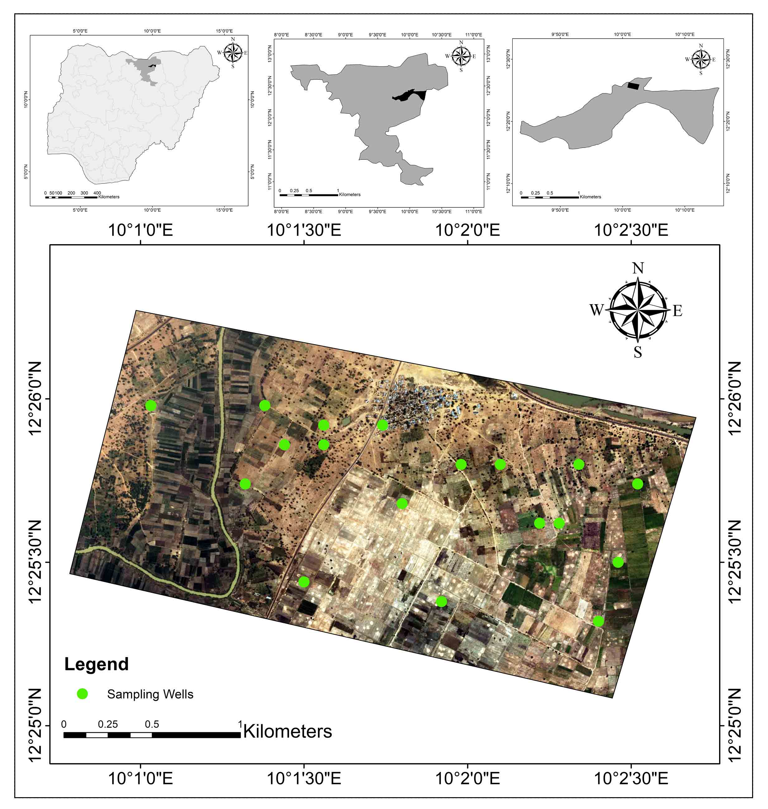
Hadejia is positioned precisely from 12º 25ʹ 10" to 12º 26ʹ 15" N latitude and 10º 0ʹ 0" to 10º 2ʹ 35" E longitude (Graba et al., 2016) which constituted part of Northwestern Nigeria. The study area falls within the sedimentary basin located along the Hadejia river basin. As described by Olofin (2014) (Figure 1), rainfall in the study location is characterized by spatiotemporal irregularities with a maximum of 600 mm/year. The rainiest months are June, July, August and September, other months being the dry season. The average temperature for each month of the year is about 27.1 ºC. The warmest period of the year is from April to July, when the maximum temperature recorded is 36.7 ºC. The lowest temperature is normally recorded during the coolest period between December and January (Tukur et al., 2018). Sampling wells location within the study area is depicted in figure 1.
Figure 1. Study area with distribution of sampling wells
2.2 Geology and Hydrogeology
Chad sedimentary formation is the dominant geological formation of the area characterized by sand sediments which mostly unconsolidated and porous allowing high infiltration capacity. The nature of geological structure allows substantial storage of water in both deep and shallow aquifers. The deep aquifers which are the two top ones and the shallow aquifers found in floodplains along the river basin. Both deep and shallow aquifers serve as the primary sources of fresh water. For this reason, hundreds of tub wells were built in floodplain for over three decades thereby utilizing the shallow groundwater for both domestic and agricultural use, principally the irrigation agriculture. For this reason, agricultural activities have been intensified thereby cultivating crops in all year round.
2.3 Soil and Land Use
Two major soil types are found in the study area namely; zonal (ferruginous soil) and intra-zonal soil. The ferruginous soil type is the matured soil and covers the largest part of the area. The intra-zonal soil type on the other hand is hydromorphic soils popularly known as floodplain. Wetland is one of the unique land uses in the study area and also one of the unique environmental resources supporting the ecological and hydrological functions as well as the socio-economic activities. With the presence of wetland in the area, grazing areas has become more productive even during the dry period of the year. Similarly, wetland in the area supports diversification of agricultural activities thereby enhancing productivity and social life.
2.4 Population and Socioeconomic Activities
Hadejia constituted almost 30% of the state’s teaming population. The dominant population consists largely of farmers. Agriculture, principally irrigated agriculture is the dominant socioeconomic activities in the area. Agricultural production especially the field crops and vegetable crops have substantially increased after the commencement of Hadejia Irrigation Scheme (Figure 1). This was achieved by harnessing the abundantly groundwater resource occupied in shallow aquifers through building of tube wells, open wells and digging of deep boreholes. This is because the water is close to the surface (<10 m) and the technique is simple and cheap for the farmers. Field crops (cotton, date palm, wheat, rice, maize, soybeans, onion, Irish potatoes, sweet potatoes, tomatoes, pepe, cherie, garen eggs, green beans, cucumber, okro groundnut, etc.), fruit crops such as sugarcane cowpea, corn, citrus, watermelon, etc. and vegetables (cavage, salat) are cultivated in the floodplain utilizing groundwater from shallow wells.
3 . MATERIALS AND METHODS
3.1 Field Measurements
Field measurement was achieved by establishing transects running in perpendicular direction to the river direction starting from points near river, middle field and end field points away from the main river. On each transect, 3 wells were selected representing near river, middle field and end field sampling points. The study adopted and used pumping test technique because it is reliable and most commonly used (Streett, 2011). A water pumping generator was used at a constant rate to pump water from the tube well’s aquifers at regular time interval within a day (early morning hours when the irrigation activities have commenced, peak irrigation hours at noon and evening hours). This was adopted to ensure a true estimation and maximum sustainable yield of the aquifer. In each tube well, a bucket of uniform capacity (15 L) and stop watch, respectively, were used to measure the volume of water pumped from the aquifer and the actual time at which the bucket is filled with water from the beginning of pumping. At each monitoring hour (morning and evening), the measurement was repeated 4 times at 15 minutes interval when the level of groundwater from the aquifer is said to be at dynamic (pumping) level. In each sampling point, the water pumping generator was used at a constant rate with a view to have a true variation of the aquifer’s sustainable yield. Each well was geo-referenced using a Germin Global Positioning System (GPS) model 72H by taking its coordinates. Furthermore, the name of the owner of each tube well was collected and an identity number was given to each tube well for easy identification during the main field activities.
3.2 Multivariate Statistical Analysis
Statistical computations provide a descriptive framework and explanations of spatial relationships, spatial differences, and spatial similarities between individual and group of variables through various statistical models (Suleiman et al., 2020). Various statistical models such as descriptive statistics, correlation and regression modeling, differences and variations models including multiple linear regressions, principal component and factor analysis, discriminate analysis, cluster analysis structural equation modeling artificial intelligence, artificial neural network (ANN) and fuzzy logic are used in addressing groundwater issues (Gaya et al., 2020). The combined use of these statistical techniques provides a holistic and comprehensive analysis of water samples by understanding the differences, relationships and variations scenarios both spatially and temporally (Al-Mukhtar and Al-Yaseen, 2019). The result outcome of the combined models is more reliable and perfect (Isikanye et al., 2018).
In this study, the hypothesis was tested using ANOVA and Pearson product moment correlation. Two-way Analysis of Variance (ANOVA) between locations and time was conducted to test the research hypothesis stating groundwater yield between morning and evening hours have no significant difference. There is no significance difference in the yield of wells between morning and evening hours. Normality test was performed on the data and found no suitable for parametric statistical test.
CA is one of the data reduction techniques that reduces and classifies data into homogenous groups popularly known as cluster. This is achieved by grouping similar and dissimilar variables in a homogenous group based on their similarities in behavior (Tukur et al., 2018). In this research, cluster analysis was applied to the groundwater yield and dynamic level with a view to grouping sampling points based on their similarities so as to reduce the number of sampling points in the future study. The reduction in the sampling points will be more economical without losing any significance of the outcome. Groundwater yield and dynamic level varies in spatial and time dimensions. 2-way ANOVA was applied to the spatial and diurnal variation of groundwater yield and dynamic level at the sampling site. Two-way ANOVA is one of the parametric statistical models that test and explains the statistical differences in data that is normally distributed (Narany et al., 2014). Two-way ANOVA was used to understand and provide the justification variables that cause the spatial and diurnal differences in groundwater yield and dynamic level. For modeling the spatial variations, 18 wells were sampled. The diurnal variation was the morning and evening hours. Correlation test was also used to test the hypothesis of the relationship between groundwater yield and dynamic level in the study locations. Five percent (5%) level of significance was used to test all the formulated hypotheses. In other words, acceptance or rejection of the hypothesis was done at 95% confidence level.
3.3 Geospatial Analysis
Geographic Information System (GIS) is considered as the essential and valuable tool in groundwater studies globally (Abdullahi and Pradhana, 2018). The application of GIS in groundwater studies can be seen in so many aspects. GIS is used in identifying and mapping areas of contaminated plumes within an aquifer (Narany et al., 2018) and delineate and map out suitable zones for utilization (Adhikary et al., 2015). Moreover, GIS is useful in providing information on the groundwater quality condition which can be used for the water management and sustainable programs (Neshat et al., 2013; Narany et al., 2014; Narany et al., 2018). In addition to these, GIS can identify and provide useful information on the potential groundwater recharge areas. Having computed the groundwater yield and dynamic level, GIS-based software was used to generate map showing the spatial variation of both groundwater yield and dynamic level from the sampling wells. This was achieved by using geostatistical analysis through krigging approach by considering near observations with similar pattern and behavior (Narany et al., 2018).
4 . RESULTS
4.1 Diurnal Variation of Groundwater Yield
Result obtained from pumping tests for diurnal variation of groundwater (Table 1) shows the minimum and maximum well yield as well as their average yield for both morning and evening hours. Well yield during morning hours ranges between 1.9 L/s (minimum) to 3.4 L/s (maximum). This could be attributed to the positions of tube wells with respect to river location, depth, etc. indicating that the depth and closeness of tube wells to the river do influence the yield capacity. Evening hours also recorded a similar variation of 3.3 L/s average yield. This shows that, the aquifer have a wide variation in their yield capacity both in morning and evening hours, respectively accounting for 44.07and 55.93 % of the total yield in the day.
Table 1. Diurnal variation in groundwater yield
Time
Diurnal variation (L/s)
Minimum
Maximum
Average
%
Morning
1.9
3.4
2.6
44.07
Evening
2.3
4.0
3.3
55.93
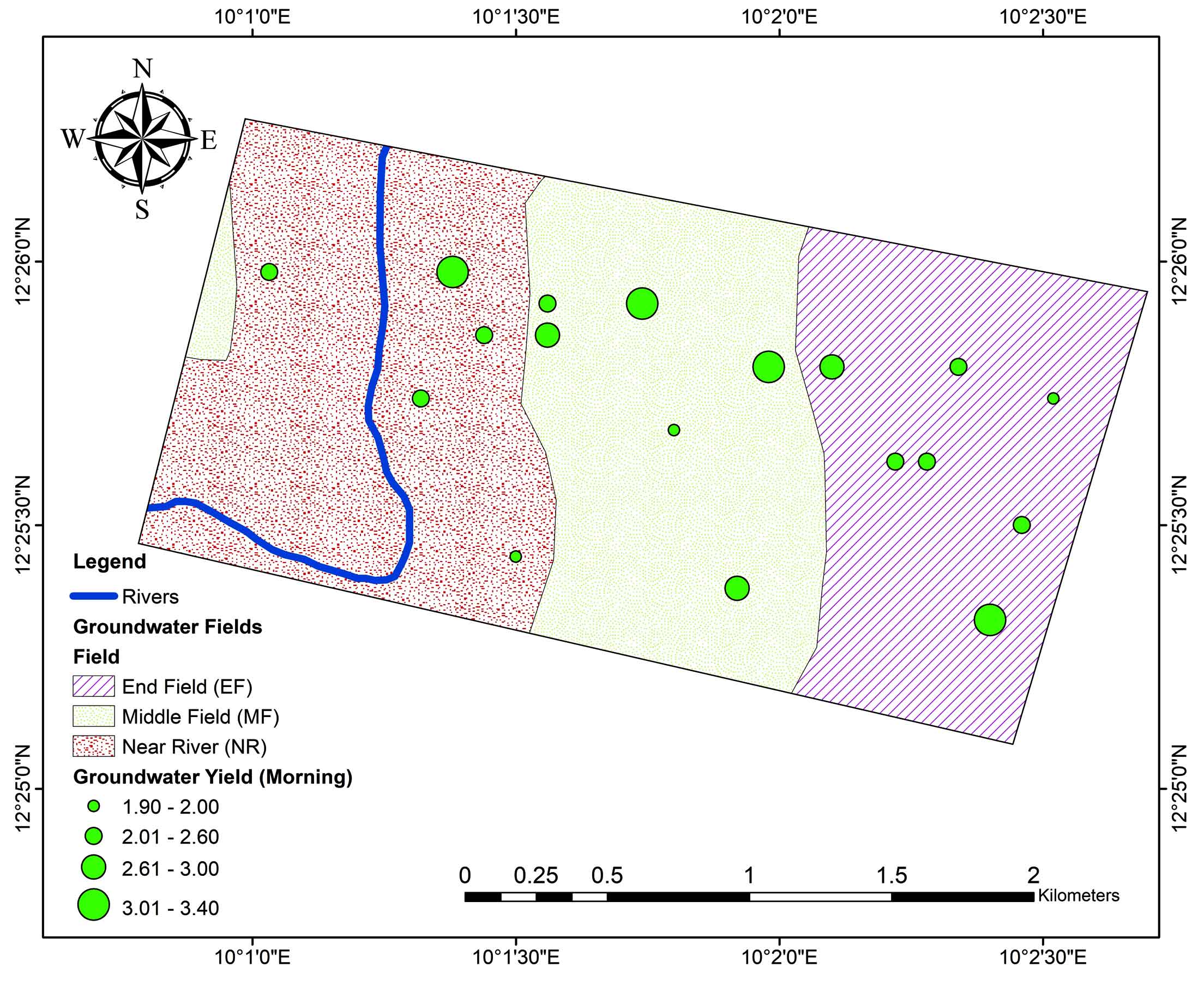
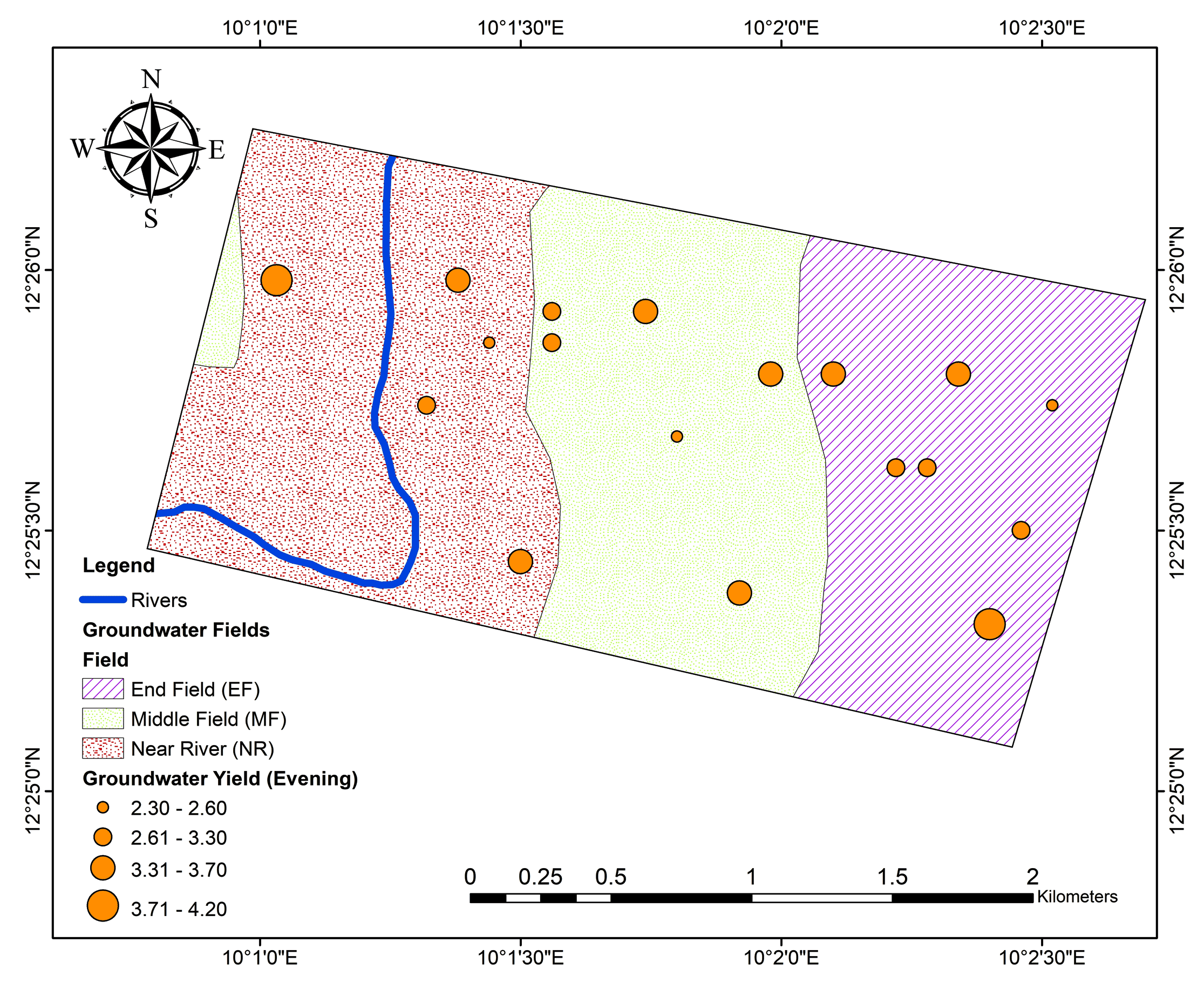
Generally, yield of wells in morning hours is lower (44.07%) than the yield of well in the evening period (55.93%) (Figure 2 and 3). Thus, there is a difference in the yield of wells between morning and evening hours. In the morning period, farmers apply water to their crops at different hours in order to make the soil wet adequately to enable crops have enough moisture. In addition to this, herdsmen always make use of groundwater from shallow aquifers in floodplain during their grazing activities for watering their animals. Interview with the well owners, revealed that the yield of some tube wells in floodplain increases with the increase in pumping. In other words, the more time taken for pumping water during the day time, the higher is the yield of the well. For this reasons, yield in morning hours is generally lower that the yield in evening hours.
Yield of wells showed no significant diurnal difference (p value, 0.00<0.05) as revealed by two-way ANOVA test conducted. In conclusion, groundwater average yield in the floodplain is still under the acceptable standard for irrigation (2.5 L/s).
Figure 2. Spatial distribution of groundwater yield: Morning hours
Figure 3. Spatial distribution of groundwater yield: Evening hours
4.2 Variation of Groundwater Yield
Impact of surface water (like the one in river) on groundwater yield is a critical issue in irrigated watershed of semi-arid regions (Helmus et al., 2009). In view of this, spatial variation of groundwater yield was modeled with a view to know whether the river has an influence on the yield of tube wells. This was achieved by sampling tube wells position with respect to distance away from river. Thus, tube wells positions within 30 to 40 meters, 500 and 1000 m away from river was named Near River (NR), Middle Field (MF) and End Field, respectively. Yield of tube wells in each field was measured both in morning and evening hours throughout the field wok activities.
Table 2 shows the spatial variation of groundwater yield for both morning and evening hours. Yield of tube wells near river and middle field recorded a similar minimum (2.5 L/s) and maximum yield (3.4 L/s), respectively, with a mean value of 2.83 and 2.90 L/s, each accounting for 36% of the total yield. The yield of tube wells in the end field positions recorded the minimum average yield of 2.23L/s, accounting for 28% of the total yield. The same model was repeated in the evening hours of irrigation activities with a view to finding out if there could be a difference from the model result of morning hours. This is because of results in table 2 shows that the yields of wells recorded in the evening hours were found to be higher than the yields recorded in the morning hours. Table 3 shows the output of the model for the yields in the evening hours. Output of the model revealed somewhat similar well yield variation as obtained in the morning hours across near field, middle field and end field positions. In other words, wells positioned in the near and middle field were found to have the highest average yield capacity (36%), followed by end field wells (28%). The result, subjected to 2-way analysis of variation, showed no significant difference in the groundwater yield related to wells positions relative to river location (p-value, 0.30 > 0.05) in morning hours.. Thus, wells positions relative to river location have no significant impact on the yield of these wells.
Table 2. Variation in groundwater yield
Well No.
Well positions
Diurnal yield (L/s)
Morning hours
Evening hours
1
Near river
2.5
4.0
4
3.0
3.3
7
2.6
2.9
10
2.9
3.5
13
3.4
4.2
16
2.6
3.6
2
Middle field
3.4
3.7
5
3.3
3.5
8
2.0
3.6
11
2.5
3.0
14
2.7
3.6
17
3.3
3.7
3
End field
2.4
3.3
6
2.3
2.5
9
1.9
2.3
12
2.4
3.2
15
2.4
2.9
18
2.0
2.6
Min.
1.9
2.3
Max.
3.4
4.0
\(\bar{X}\)
2.6
3.3
Generally, tube wells positioned in the near and middle field were found to have highest yield capacity (36%) followed by the tube wells in the end field recording the lowest yield capacity (28%).The 2-Way ANOVA at 5% level of significance showed no significant difference in the groundwater yield related to wells positions relative to river location showed no statistical significance difference as revealed by 2-way ANOVA test (p-value, 0.21 > 0.05) in evening hours. This means that, the study is 95% confident in accepting the null hypothesis. The fact that the result of ANOVA revealed no statistically significant difference between points suggests that the adopted model can be applied in other similar sedimentary basins with a view to validating it.
4.3 Cluster Analysis of Groundwater Yield
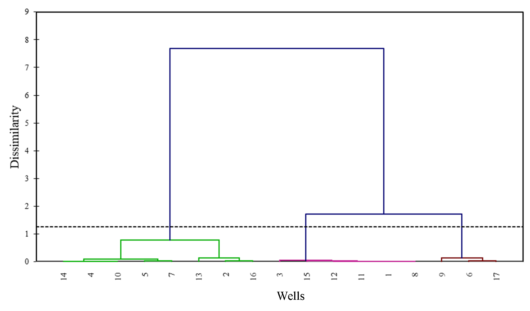
The result rendered a dendrogram as shown in figure 4, grouping all the 18 sampled wells into four statistically significant clusters: Cluster 1 (well 4, 5, 7, 10 and 14), cluster 2 (well 2, 13 and 16), cluster 3 (well 3, 12 and 15) and cluster 4 (well 1, 6, 8, 9, 11, and 17). The dendrogram grouped all wells positioned in near river and end field in cluster 1. Similarly, wells in cluster 3 are all positioned in end field of the river. This suggests that wells grouped in one single cluster have similar yield capacity. Therefore, instead of monitoring groundwater yield from all the 18 wells, only four sites would be selected in future spatial sampling without affecting the result adversely. In other words, instead of selecting all the wells belonging to one cluster, only one well from each cluster would be selected.
Figure 4. Dendrogram clustering similar and dissimilar sampling wells for groundwater yield
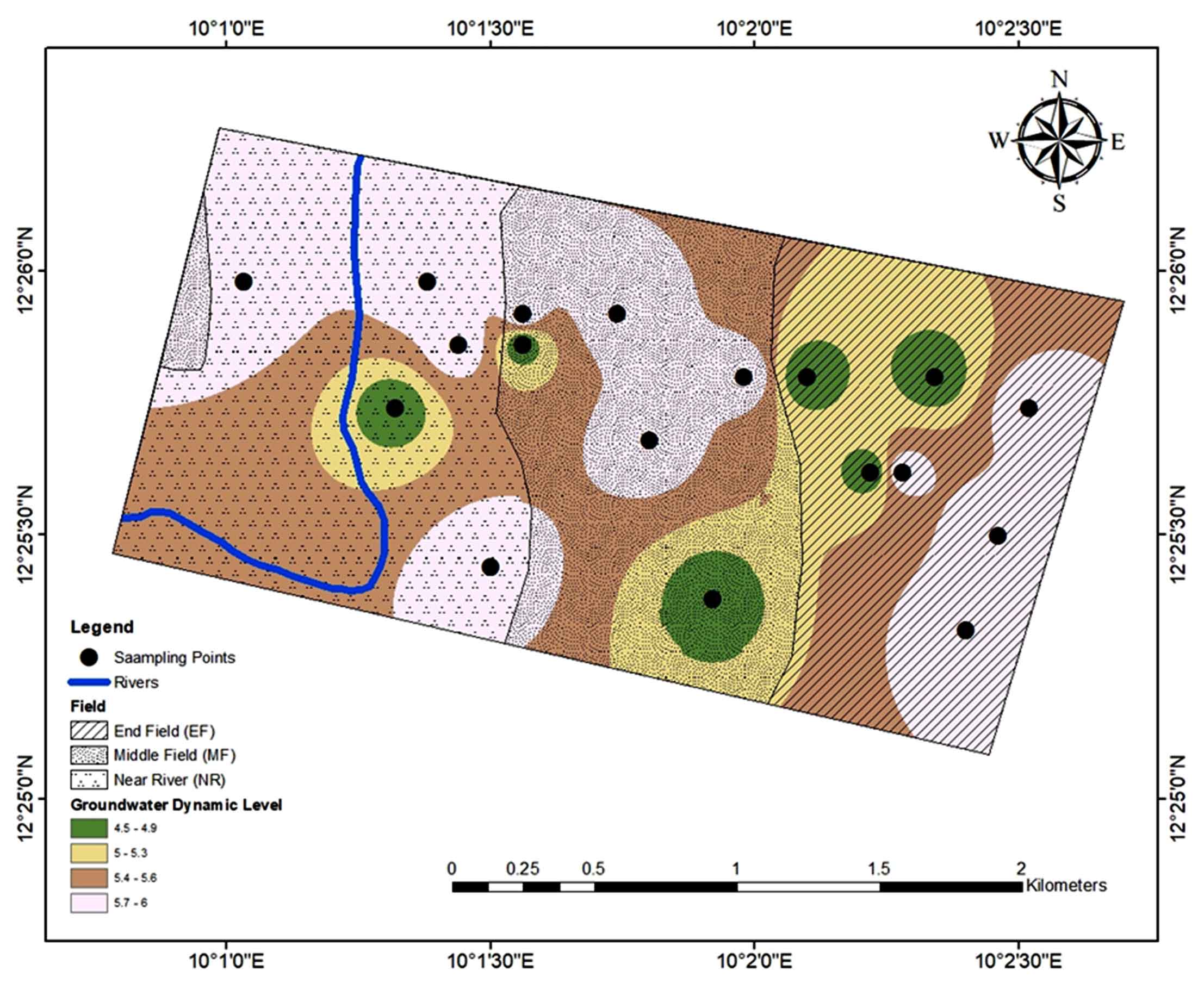
4.4 Variation in Groundwater Dynamic Level
Dynamic level of groundwater was determined in the field for the following reasons: to ensure a true estimation and maximum sustainable yield of the aquifer; to find out where the groundwater level varies with respect to distance away from river; and to know whether groundwater level has a relationship with the yield. Table 3 shows the spatial variation of the groundwater dynamic level in the study area. Model output shows that, groundwater dynamic level varies from 4.5 to 6 meters, with an average level of 5.0, 5.5 and 6.0 meters in the wells positioned near river, middle field and end field, respectively. Thus, the dynamic level of groundwater in the wells varies with the positions of the wells relative to the river such that those in the end field recording the maximum (Figure 5). This indicates that the level of groundwater lowers with distance away from the river in the area. The dynamic water levels in wells positioned in the end field have higher depths of about 36.4% more than those in the middle field (33.3%) and near river (30.3%), unlike in the case of yield capacity of wells located in the near field recorded the highest yield capacity.
Table 3. Variation in groundwater levels
Well No.
Well Positions
Dynamic Water Level (m)
1
Near River
6
4
4.5
7
4.5
10
4.5
13
6
16
4.5
2
Middle Field
6
5
6
8
6
11
4.5
14
4.5
17
6
3
End Field
6
6
6
9
6
12
6
15
6
18
6
Min.
4.5
Max.
7.5
\(\bar{X}\)
5.5
Groundwater dynamic level with respect to river location shows no significant spatial difference (p-value 0.842 > 0.05) as revealed by 2-Way ANOVA test. Pearson product moment correlation test at 5 % level of significant was used to test the relationship between groundwater yield and dynamic level. The result revealed that there is significant relationship between groundwater dynamic level and yield (p-value, 0.045 < 0.05). In other words, groundwater dynamic level has good relationship with the yield in the floodplain of Hadejia.
Figure 5. Spatial variation of groundwater levels
5 . CONCLUSIONS
A combination of painstaking measurements and multivariate statistical modelling was used to develop a model explaining the relationship between groundwater yield and the dynamic level of water in a nearby river. Although average yield of groundwater in the morning hours is lower (44.07%) than in the evening period (55.93%), but they falls under the acceptable standard for irrigation based on FAO (1998). Model outputs of 2-Way ANOVA shows no significance spatial difference (p-value, 0.21 > 0.05) in the yield of wells with respect to river location. However, the diurnal difference in the yield of wells shows statistical significant difference (p value 0.00 < 0.05, suggesting the impact of time differences on groundwater yield. Relationship between groundwater yield and dynamic level was to be significant (p-value, 0.045 < 0.05). Furthermore, since this study is a sort of a pioneering research of its kind, it is recommended that the study should be replicated in other parts of the study area as well as other sedimentary structures in similar environments to validate the findings of this study.
6 . FUNDING AGENCY
Authors sincerely thank ‘Tertiary Education Trust Fund’ for sponsoring the whole PhD work during year 2016-2018 of which this paper was developed.
Tables
Figures
Conflict of Interest
The authors do not have any conflicts of interest.
Acknowledgements
We sincerely thank Mr. Suleiman Damban of the Department of Geology, Hadejia River Basin Development Authority, Kano, Nigeria for his guidance on measuring groundwater yield. We also thank Muhammad Abdulkadir and Muhammad Ibrahim Fantai for their assistance during field work measurements. We acknowledged the contribution of Mr. A.W. Tende of the Department of Geology, Kano University of Science and Technology, Wudil, Nigeria for GIS analysis made in this study. Lastly we thank Emeritus Professor E. A. Olofin for vetting the manuscript.
Abbreviations
ANOVA: Analysis of Variance; CA: Cluster Analysis; GIS: Geographic Information System; MDG: Millennium Development Goals; UNESCO: United Nations Educational; Scientific and Cultural Organization.
Iliya, M. A., Muhammad-Baba T. M ., and Oppon-Kumi, A., 2011. Climate change, land degradation, forced migration and farmers- pastoralists conflicts in the Sokoto-rima basin in north-western Nigeria: observation and extrapolations. First National Conference on Climate Change, 24th May, 2011, Bayero University Kano, Nigeria
Mays, L. W., 2009. Integrated urban water management: Arid and semi-arid regions, Tylor and Fransis Group plc: Leiden, The Netherlands, UNESCO Publishing, Paris, France, 1-73.
Olofin, E. A., 2011. Geographical hydrology lecture note series, Department of geography, Bayero University, Kano, 3-4.
25.
Olofin, E. A., 2014. Location, relief and landform. In (Ed.) Tanko and Momale, Kano: Environment, society and development, Adonis and Abbey, London and Abuja, 1-11
26.
Olofin, E. A., 2016. Water resources planning and management: lecture notes on WMA501: Water resources planning and management, Department of Water resources management and agro-meteorology, Federal University of Oye-Ekiti, Ikole Campus, Nigeria, 4-12.
Umar, D. A., Ramli, M. F., Aris, A. Z. and Zaudi, M. A., 2019a. Hydrological response of semi-arid river catchment to rainfall and temperature fluctuations. Pertanika Journal of Science and Technology, 27(4), 2333- 2349.


 ,
Maharazu A Yusuf 1
,
Maharazu A Yusuf 1