1 . INTRODUCTION
The developmental process has much impact on the urbanization which has been little understood. World’s urbanization has been increased from 30 to 50% between 1950 and 2010. During 2010, the urban population of the earth touched the mark of 350 million which intersect the 50% smudge. Developing countries in Asia and Africa do not show any insignia of lower down and sustained growth is evident (Duong, 2014; Herold et al., 2002). Developed countries concentrated with 78% of the urban population where the figure turns into 52% for the developing countries. Urban centers having more than 0.1 million population are facing tremendous pressure of population influx compare to previous decades (McDonnell et al., 2008; Nageswararao and Narendra, 2006). In Asia, 30% of urban area possessed with 60% of urbanites with 42.2% urbanization rate in 2010.
Spatiotemporal influence of emerging large cities in connectivity, trade and utility services and amenities aspect pull rural population a movement towards urban areas in a haphazard manner or in a planned way (Hester et al., 2008; Long et al., 2007). This rapid growth and population concentration resulted in the horizontal expansion of urban space within its limit in great extent and the phenomenon of such growth is commonly reflected as urban sprawl (Li, 2009; Martin, 2003; Liu et al., 2014). Nature of spatial transformation within a particular timeframe echoes the nature of urban growth process (Bhatta et al., 2010; Huang et al., 2007).
Therefore, it can be argued that urban growth and sprawling can be considered as spatiotemporal process of an area. Appraisal on the spatial and temporal context directed to conclude that so many scholars have observed this system as a complex process (Kim and Batty, 2011; Sudhira et al., 2004; Cheng and Master, 2003; Weerakoon, 2017).
Advancement in remote sensing and GIS with the integration of land science provided a great podium to perform and scrutinize the changing nature of the landscape in spatial and temporal dimension (Estoque et al., 2014; Gutman et al., 2004; Turner et al., 2007). Inspect about the driving factors associated with landscape change with descriptive statistics are noteworthy when size and speed of changing land use are concern (Hersperger et al., 2010; Plexida et al. 2014). With such consideration, assessment of spatial and temporal urban growth will be helpful (Long et al., 2007; He et al. 2013; Estoque et al., 2014). In the study of landscape ecology, urban gradient has been often used to characterize the spatial and temporal extent of urban transformation (Luck and Wu, 2002; Estoque and Murayama, 2012; Estoque et al., 2014). Several researchers pay their attention in landscape spatial metrics to characterize the landscape assembles and spatiotemporal design of urban setting (Estoque and Murayama, 2016; Aguilera et al., 2011; Wu et al., 2011). Based on fractal geometry and information theory, urban spatial metrics has been developed for the study of urban spatial structures and spatiotemporal pattern of urban land transformation in a very effective manner (Mandelbrot, 1989; Estoque and Murayama, 2015; Agrilera et al., 2011; Wu, 2011; Plexida et al., 2014).
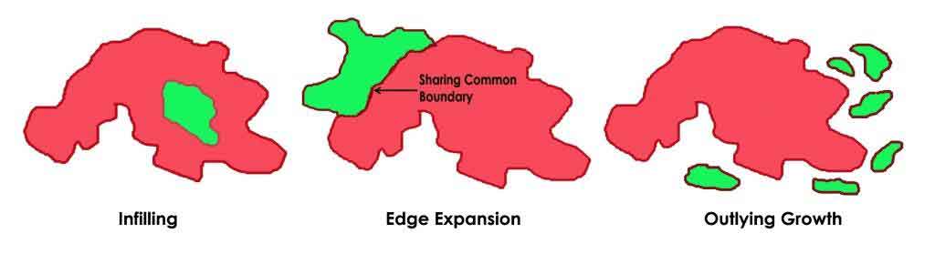
Many researchers pointed out the phenomena of urban sprawling and haphazard growth in developing countries found tremendous during last few decades and the tendencies of dispersed expansion impede a serious problem for the modernization and wellbeing of the society (Rahaman, et al., 2011; Ramachandra et al., 2012). Presently, the measurement of urban sprawl is one of the burning topic of investigation. Remote sensing data and GIS techniques can apply for the study of urban sprawl in combine. (Dietzel et al., 2005; Dewan and Yamaguchi, 2009; Herold et al., 2002). Before the application of RS and GIS on sprawl quantification, the researchers must know the typology of urban expansions which is basically three types in nature (Li, 2001; Li and Reynolds, 1993; Hester et al., 2008). Urban expansion happens either with the same population density, or reduced density or increased density. New developments through the infill process or redevelopment of the existing built-up area make a change of urban density (Weerakoon, 2017; Kamini et al., 2006; Herold et al., 2005) and recognized three types of urban growth pattern which have been termed as: infilling, edge expansion and outlying growth. Earlier three major forms of urban growth pattern have been addressed by Harvey and Clark (1965) as low-density continuous growth, ribbon development and leapfrog development. As there was no quantification done by Harvey and Clark, it was really tough to separate low-density continuous growth from ribbon development or leapfrog development. Liu et al. (2010) have noted three growth types in urban growth monitoring, namely infilling, edge expansion and impulsive growth using Landscape Expansion Index (LEI). The LEI value ranges from 0-100. 1-50 LEI represents infill growth where 50-100 represents the edge expansion. Outlying growth or spontaneous growth can be found when LEI is zero. LEI ranges from 0 to 1, where ‘0’ represents spontaneous growth, 0-0.5 signifies the edge expansion and above 0.5 representing the infill growth pattern. This approach has been found on Hanoi, Vietnam where Nong et al. (2014) measured the spatiotemporal urban growth patterns.
Recognition on the typologies of urban growth can be measured through LEI but the expressive picture may be the limitations until this result put forward along urban-rural gradient using buffer analysis. Landscape pattern in the urban regions usually changes through the process of haphazard urban growth. In this period, heterogeneity of the land has been found in decreasing nature with increasing landscape fragmentation with an increasing number of smaller patches. Such changes in an urban area can be identified using spatial metrics and categories the complex landscape structure into a simple and identifiable pattern (Ji et al., 2006; Jenerette and Potere, 2010). In natural vegetation, landscape and spatial metrics have been used frequently (Gustafan, 1998; Hargis et al., 1998; McGarigal et al., 2002; O’neill et al., 1998). Application to the field of research outside the landscape ecology and across different kind of environments, this approach is suitable for urban areas which are more generally termed as ‘spatial metrics’. Different indices (on the basis of patch and pixel) such as size, shape, edge, diversity can be assessed using the spatial matrix for an urban area (Gustafan, 1998; Martin, 2003). Several researchers have been categorized and developed a significant set of urban metrics to study the important aspects of urban landscape pattern (Cushman et al., 2008; Ritters et al., 1995). After an intense literature survey, eight spatial metrics have been selected to study the urban landscape fragmentation.
During the past two decades (i.e. 1996-2006 and 2006-2016), Howrah Municipal Corporation (HMC), India has experienced an enormous growth of the urban population. During 1980s, HMC undergone various developmental stage and then Howrah municipality has been transformed as HMC. After 1984, the rapid growth of urban population took place due to its industrial competitiveness, network facility and nearness of Kolkata city. During 2001-2011, the concentration of census towns (basically small size urban centers) in Haora district accounted nearly 10% of State’s census town which presents a clear picture of the spontaneous growth of urban area not only from farm to non-farm transformation but also due to migration from rural to an urban area. This argument has also been validated from 2011 census data where the rural population growth has shown a negative growth pattern. Present study analyses the urban growth pattern and urban form of HMC, India. The primary objective of the study is to assess the varying speed of urban built-up growth during 1996-2016. After assessing the above mentioned objective, growth types in urban-rural gradient and spatiotemporal analysis of urban growth patterns has been quantified using spatial metrics for HMC and its surroundings during 1996-2016.
2 . STUDY AREA
Howrah is a commercial and industrial city of West Bengal, India developed alongside its twin city Kolkata. HMC is the headquarters of Haora district and positioned on the western bank of River Hugli. Presently the city gains more importance as a principal administrative unit - State Secretariat ‘NABANNA’ is located within the city’s jurisdiction. It is the third largest city of West Bengal after Kolkata and Asansol. Howrah is famous for busiest train terminal and this city also having Santraganchi and Shalimar train terminals. This city connects with Kolkata with several bridges, e.g. Vidyasagar Bridge, Howrah Bridge, Bally Bridge within a short span of time. Though the district of Haora has a long history of urbanization, Howrah and Bally were the only two urban centers till the independence of India. But after 1947, the pace of urban expansion was reasonably faster and as a result, Haora district achieved 53 towns in 2001. During 2001-2011, the unprecedented growth of census towns (nearly 25% urban centers of the district total) makes the researchers more interested in study the urban pattern of the district.
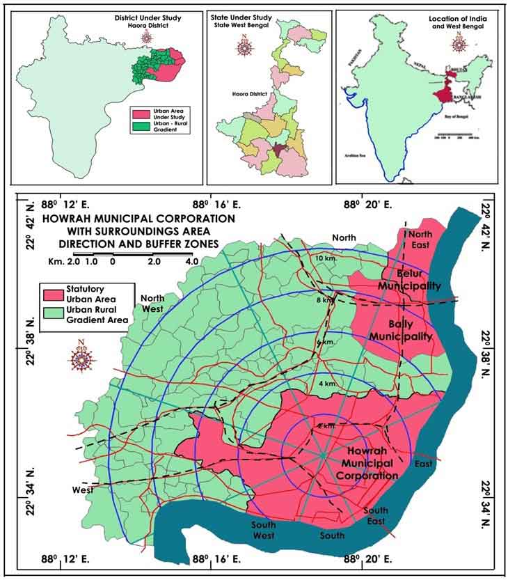
The study focuses on HMC and its surrounding area (Figure 1). Howrah municipality was established in 1862 with an area of 50sq.km. Howrah municipality became HMC in 1984 with 50 wards distributed among 7 borough offices for the operation of daily work. HMC extends from 88°12ʹ16ʺ E. to 88°21ʹ36ʺ E. longitude and from 22°33ʹ30ʺ N. to 22°41ʹ08ʺ N. latitude with approximately 51.74 sq.km area with 10,77,075 population with a sex ratio of 919 in its civic boundary.
The working structure and composition are very high in this municipality because a huge migration from rural to urban took place constantly (Census of India, 2011). Within its 15 km buffer, HMC experience nearly 30 census towns among 72 numbers (nearly 10% of State’s Census Town) concentrated in the district during 2001-2011. The reasons behind the selection of HMC as units of research in respect of urban growth are basically threefold in nature as:
- The district has experienced a huge number of census towns during 2001-2011 (5% share to state).
- As Howrah city is known as ‘Sheffield of India’ for its industrial dominance, this urban agglomeration has lopsided pattern of urban growth. As a result, the expansion of the city might follow the sporadic pattern of urban growth which influences sprawling pattern: infilling, edge expansion and spontaneous growth.
As through railway and road network accessibility, it is very near to Kolkata, which is state capital and most important industrial, commercial, administrative, education and health hub. Nearness of Kolkata makes an urban shadow to Howrah and its surroundings which make more prospective for urban growth.
4 . METHODS
4.1 Built-up Growth Index
The Enhanced Built-up and Bareness Index (EBBI) is based on the indexing of remote sensing data which is a combined effect of Near Infra-Red, Short Wave Infra-Red and Thermal Infra-Red (0.83μm, 1.65 μm and 11.45 μm, respectively) of Landsat image. Herold et al. (2004) analyzed built-up reflectance posing higher values due to having longer sensor wavelengths. NIR and SWIR band show high spectral values of built-up (i.e. urban, concrete roof, roads, walkway, flyover etc.) and bands give an inverse reflectance ratio to vegetation and water bodies. For mapping the built-up areas, TIR channel is one of the effective channels (Weng, 2008) which confirm 10-12 degrees lower than the built-up environment. To achieve a higher degree of built-up effect, an improved mathematical operation has been followed (Rahman et al., 2012). To find out the EBBI, the following formula has been used which is applicable for Landsat 5 and Landsat 8:
\(EBBI = {Band \ 5- Band \ 4 \over 10 \sqrt{Band \ 5 + Band \ 4}}\) (1)
As this analysis has focused only on urban change, landscape heterogeneity was simplified and three basic maps have been developed: i) built-up (urban footprint) that exist before 1995, ii) urban change during 1995- 2005 and iii) urban change during 2005-2015 and here other land cover classes such as water bodies, green belt and open space have been ignored. The overall methodological pattern of the study is shown through a flow diagram (Figure 2).
Table 3. Results of Enhanced Built-up and Bareness Index (BEEI) with Accuracy
| Sensor |
Years |
Classified Image |
Overall accuracy |
Kappa Statistics |
| Landsat TM |
1996 |
Enhanced Built-up and Bareness Index (BEEI) |
92.13% |
0.931 |
| Landsat ETM |
2006 |
Enhanced Built-up and Bareness Index (BEEI) |
93.87% |
0.907 |
| Landsat ETM+ |
2016 |
Enhanced Built-up and Bareness Index (BEEI) |
95.31% |
0.942 |
4.2 Typology of Urban Growth along Urban-Rural Gradient
The basic three pattern of urban growth has been quantifying using Landscape Expansion Index (LEI) (Figure 3). It is basically the ratio of earlier urban footprint to newly grown urban patches. When spatiotemporal urban growth pattern is a concern, LEI is an important methodology to analyses the landscape change. The LEI has been calculated using the formula (equation (2)) as derived by Liu et al. (2010):
\(LEI = LC/ p\) (2)
where, LEI = Landscape Expansion Index, LC = length of common boundary and p = perimeter of the newly developed built-up area.
Area-Weighted Mean Expansion Index (AWMEI) (equation (3)) has been calculated to understand the virtual control of different urban arrangements in the spatial or temporal frame.
\(AWMEI= ∑^n_{(i-1)} LEI_i \times ({a_i \over A}) \) (3)
where, \(LEI_i\) is the outcome of Landscape Expansion Index for the patch which have formed newly, i.e. ‘I’, ‘\(a_i\)’ is the new patch area and ‘A’ is the total area of grown patches formed newly.
When AWMEI is found with higher results it imply the compact pattern of urban form and lower the results agrees to occurrence of leapfrogging or spontaneous growth (Liu et al., 2010; Dietzel et al., 2005). After having the result of LEI and AWMEI, buffer gradient analysis has been done (Table 2). Five buffer zones having 2km interval from the core of HMC in eight directions has been developed to study the urban-rural gradient. Within each buffer of each direction landscape expansion categories and spatial metrics has been analyzed in the next part to understand the changing characteristics along the urban-rural gradient.
4.3 Quantifying Spatial/ Landscape Metrics
Landscape spatial metrics or indices are the representation of quantitative indices to portray the structures and pattern of urban growth (McGarigal and Marks, 1995). Here, some of the indices have been used which have explicit meanings in relation to behaviour of urban patches i.e. dispersal or amalgamation (Lei and Wu, 2004; Seto and Fragkias, 2005). In this study, changing urban pattern has been analyzed using a set of selected landscape metrics. The landscape metrics has been quantified with open source software using FRAGSTAT version 4.3 (Mcgarigal et al. 2002). Selected metrics (Table 2) have been considered using \(30 \times 30 m\) cell neighbourhood rule in FRAGSTAT software for each level classification map and then the results have been evaluated.
4.4 Selected Landscape Metrics for Urban Pattern Analysis
4.4.1 Class Area (CA)
Class area is the spontaneous metrics castoff to analyze the arrangement of urban growth in the frame of spatial metrics. Sometimes it is recognized as total area covered by a land cover class in hectares (McGarigal and Marks, 1995). ‘CA’ value ranges always greater than ‘0’ and extent up to without limit. Class area and the total area will be the same value during the complete landscape comprises in a single patch as a compact urban unit.
4.4.2 Number of Patches (NP)
Number of patches determines the discontinuity of discrete growth in the urban setting. Number of patches grows in a huge number during the rapid urban growth which is basically located around the nuclei. NP is a sign of the landscape diversity and its richness. The number of patches measures urban expansion when the landscape gets more fragmented and heterogeneous. ‘NP’ value ranges always greater than 1 and extends up to without limit. When the urban setting contains with single patch, NP becomes ‘1’.
4.4.3 Patch Density (PD)
Landscape fragmentation can also be measure by using patch density (PD) which directly indicates the distribution and density of patches of a land cover class within a specified area. Patch density is also a good indicator for landscape fragmentation. When the number of minor patches intensifies without significant growth in urban setting, PD values increases. This show a more varied and scrappy urban growth pattern. However, when the number of patches and total landscape area increases in proportionate manner, there will be no significant change in PD will be evident in urban setting. Value of patch density lies always greater than ‘0’ and extent without limit.
4.4.4 Edge Density (ED)
Edge density measures the edge length of urban patches which is another important indicator of urban expansion level. It is figure out by divide the length of the urban boundary and total urban-scape. When the edge extent of specific land cover class (urban area) increases, fragmentation nature within the urban landscape also increases (Figure 3). Here the smallest mapping unit is the pixel. An increment in NP can certainly lead to an increase in edge density (ED). Value of edge density (ED) lies always greater than ‘0’ and extent without limit.
4.4.5 Largest Patch Index (LPI)
Largest patch index (LPI) is a measure of ratio lying between ‘0’ to ‘100’ and expressed in percentage. LPI is the ratio between largest urban patch and the total area in urban setting (Herold et al., 2002). LPI approaches towards ‘0’ when largest patch of the conforming patch type becomes increasingly smaller and LPI approaches found ‘100’. This index is a measure of discrete core to a dominant core.
4.4.6 Area Weighted Mean Patch Fractal Dimension (AWMPFD)
Area Weighted Mean Patch Fractal Dimension (AWMPFD) is the average value of fractal extents of the urban patches with a larger path. Metric value of AWMPFD lies within 1 and 2. Additionally, AWMPFD matches the average patch fractal dimension (FRACT) lies in the landscape, weighted by patch area.
4.4.7 Contagion (CONTAG)
Probability of neighborhood pixels of the same class can be measure by Contagion (CONTAG) as describes by O’Neill (1998). This index determines the aggregation or clumpiness of landscape. In other words, contagion is the measure of adjacency. In case of large patches within the landscape, high value with contagious patches has been evident. The lower value of contagion indicates the fragmented patches in an urban setting. The result of CONTAG lies within 0 and 100%.
4.4.8 Shannon’s Diversity Index (SHDI)
Variety of urban patches and its relative abundance in a landscape can be represented using Shannon’s entropy which is a quantitative measure. SHDI value ranges not less than 0 to without any limit. In urban planning quantification analysis of the richness in patch diversity are the key facets for landscape study.
5 . RESULTS
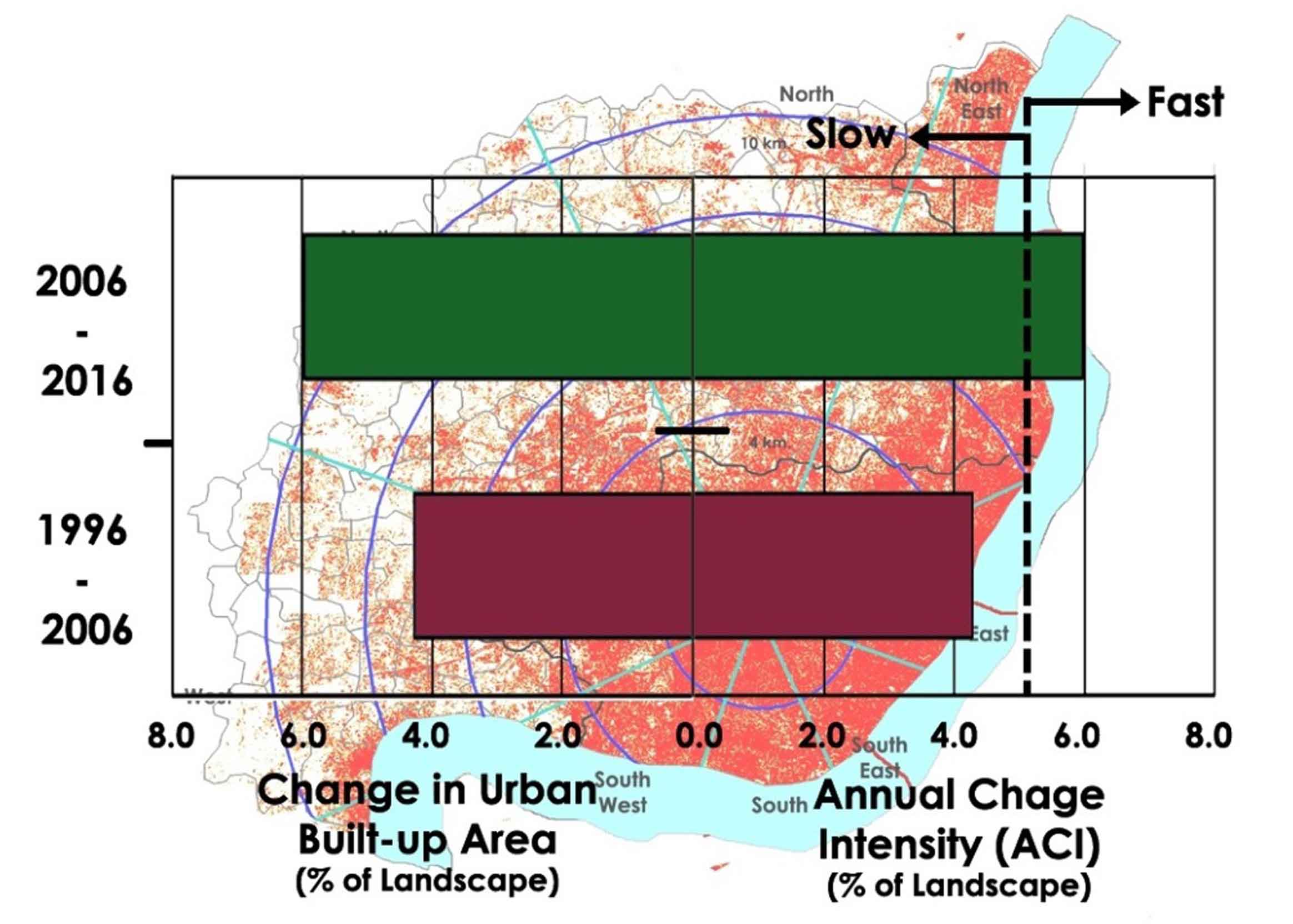
5.1 Varying Speed of Urban Built-Up Growth during 1996 - 2016
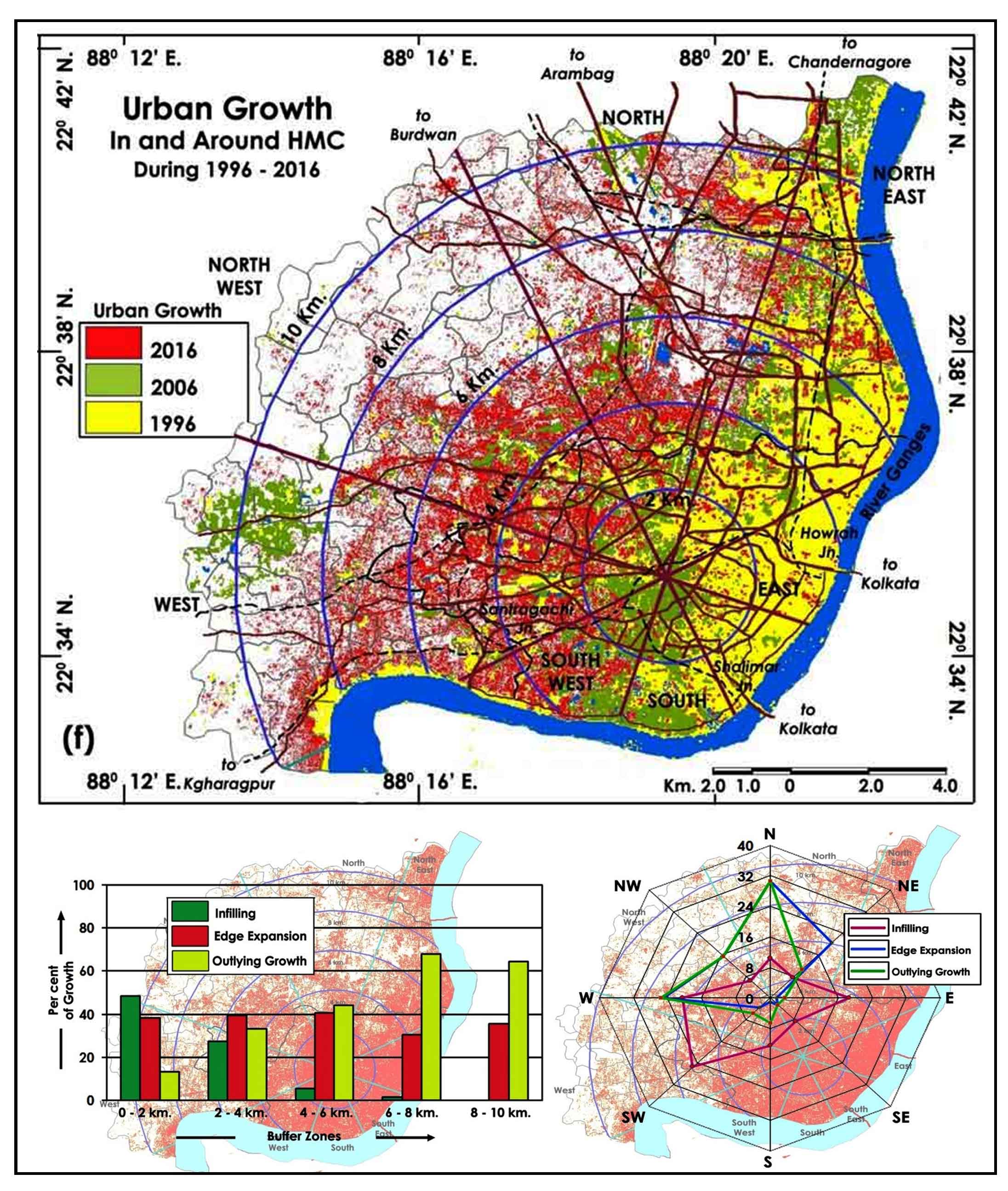
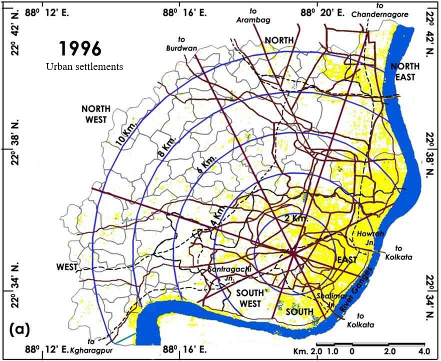
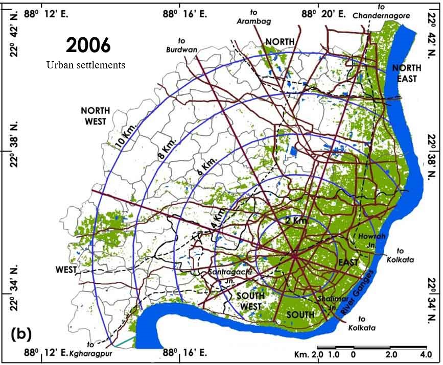
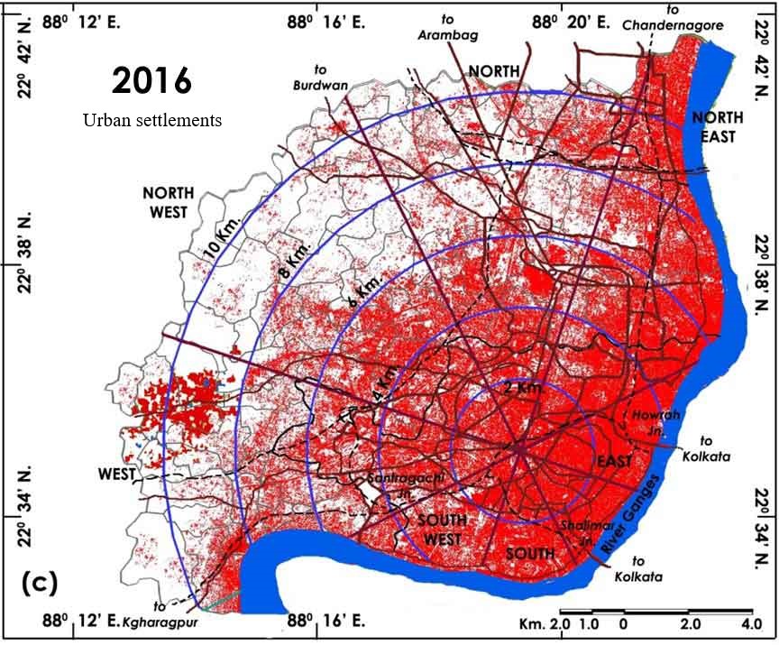
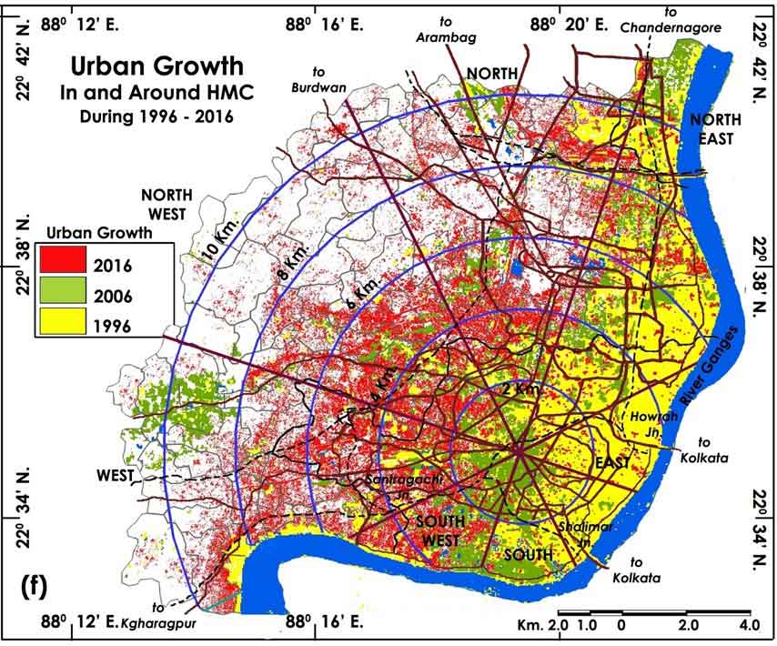
The classified EBBI map of Howrah and its 10km surroundings (from city core) of the years of 1996, 2006 and 2016 has been shown in Figure 4 (a-f) and comparative growth of built-up in Figure 5. The achieved overall classification accuracies were 92.13%, 93.87% and 95.31% and overall kappa statistics were 0.931, 0.907 and 0.942, respectively for the classification of 1996, 2006 and 2016 temporal span. Present study on Howrah and its surroundings has successfully achieved overall kappa statistics at about 92% and hence the analysis is accepted (Lea and Curtis, 2010). The classified Enhanced Built-up and Bareness Index has been summarized in Table 3.
The proposed method as defined by Rahman et al. (2011), Enhanced Built-up and Bareness Index (BEEI) has been found most accurate to extract the built-up environment of the study area. The composition of marked statistics has been marked as a growth pattern for a span of 20 years. The increase of built-up area during 2006-2016 has been found significantly to the other date (i.e. 1996-2006). The statistics for the year 1996 shows city area to spread over 4025 hectares which were increased to 5748 hectares in 2006 and 9189 hectares in 2016. The result demonstrates that HMC and surrounding areas gaining approximately 128.30% in the past 20 years (i.e. 1996-2006) at a rate of 258 hectares per year. The increase of built-up area during 1996-2016 spread over the North, West and Northwest directions, mainly. This growth pattern shows the fragmented and linear expansion along the outer peripheral portion of the study area whereas infilling pattern has found as a dominant pattern in the city core. The results from EBBI have been further analyzed using of gradient approach and spatial metrics for the better understanding the form of built-up growth.
5.2 Growth Types in Urban-Rural Gradient during 1996-2016
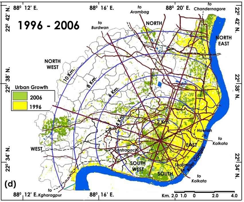
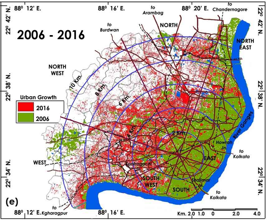
LEI in the study ranges from 0 to 1 and the urban growth types acknowledged as follows: LEI> 0.5 represents infill growth, LEI< 0.5 represent edge expansion and LEI equals to zero is termed as spontaneous growth. Figure 4 a-f shows three classified images for HMC and its surrounding areas (1996, 2006 and 2016) and detected built-up class (i.e. gaining the built-up or transformation of non-built-up to built-up environment). In the year 1996, the HMA’s built-up land was 4025 hectares which was increased into 5748 hectares in 2006 and 9189 hectares in 2016. This result shows that HMC and surrounding areas gaining approximately 128.30% in the past 20 years (i.e. 1996-2006) at a rate of 2.58 sq.km. per year. It is noteworthy that in 1996, urban built-up accounted for only 5.13% of the entire landscape, while in 2006 it was 7.33% and in 2016 turn into 11.72% of the total area. The landscape expansion index calculated different expansion types during 1996-2016 of HMC and its surroundings (Table 4). These types of urban growth has been termed as infilling, edge expansion and outlying growth. After categorizing the urban growth from Figure 4 a-f, it was further studied with LEI to determine the types of urban growth took place in HMC and its buffer area up to 10km (peri-urban-rural zone) calculated land extent in pixel and per cents are shown in Table 4.
Table 4. Types of urban growth
|
Typologies
|
1996-2006
|
2006-2016
|
|
Pixels
|
%
|
Pixels
|
%
|
|
Infilling
|
11,788
|
7.45
|
12,582
|
5.25
|
|
Edge expansion
|
62,745
|
39.65
|
87,238
|
36.40
|
|
Outlying growth
|
85,292
|
53.90
|
139,847
|
58.35
|
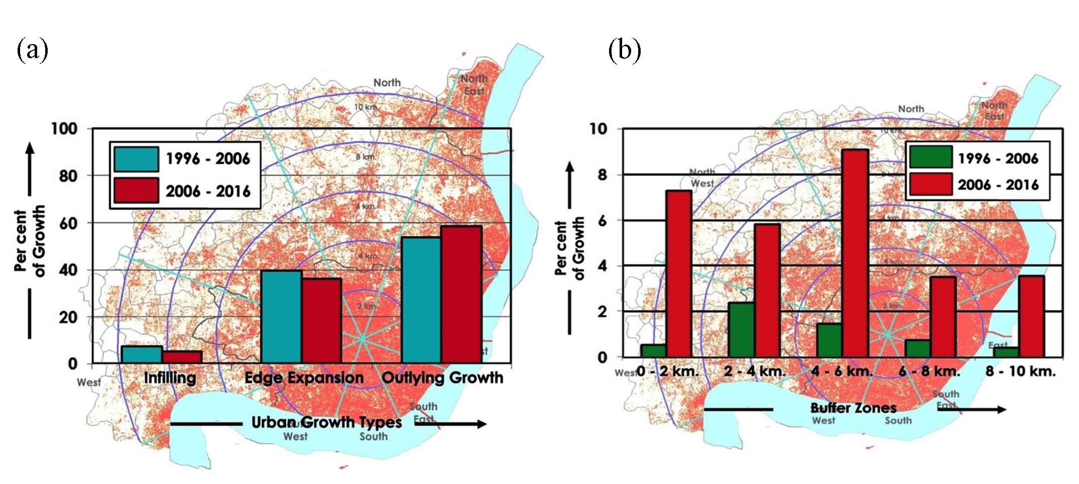
Throughout the 20 years (1996-2016) of study, outlying growth has been considered as primary growth type. During 1996-2006, infill growth has shown an insignificant percentage of 7.45 while outlying growth accounted for 53.90% (Table 4). During 1996-2016, infill growth never has shown any momentous surge. However, edge expansion accounted for such significant growth but less as it was during 1996-2006. During these two periods, the outlying growth increased by nearly 5% (from 53.9% to 58.35%). Figure 6a exemplifies the percentages of different urban growth during these two study periods. As revealed in Figure 6a, the main urban growth type during the entire study periods was outlying growth though it has been accounted for 53.9% during 1996-2006 and increased to 58.35% during 2006-2016. Infill growth has been decreased from 7.45 to 5.25%. According to Figure 7a, outlying growth and edge expansion in and HMC along SE railway and the main arterial road took place in a rapid manner. As the stimulus of three diverse types of urban growth proportionate with distance from the core of Howrah city, it is necessary to compute the usefulness of these growth types from the city core to different distance and directions. In first, the urban change during 1996-2016 in the HMC and its 10km buffer determine a gradual change of 4025 hectares to 9189 hectares which corresponds to 5.13% to 11.72% of total area. Built-up growth rate (annually) for five buffer zones during the study period has also been calculated which shows the dissimilar growth trend during two study periods (Table 5) and tends to fluctuate reliant on the distance from HMC core.
Table 5. Urban growth rate in buffer zones
|
Temporal span
|
Buffer zones
|
|
Up to 2km.
|
2-4km.
|
4-6km.
|
6-8km.
|
8-10km.
|
|
1996-2006
|
0.53
|
2.39
|
1.46
|
0.72
|
0.42
|
|
2006-2016
|
7.29
|
5.83
|
9.09
|
3.52
|
3.55
|
According to the Table 6, the average annual growth rate within the 2km buffer did not show any noteworthy change during 1996-2006 which 0.53% but during 2006-2016 it was jumped up to 7.29%. During 1996-2006, the average annual growth rates were 2.39, 1.46, 0.72 and 0.42%, respectively for different buffer (Figure 6b). During 2006-2016 similar pattern of growth has been experienced by all buffer zones except 4-6km buffer. Within 4-6km buffer the average annual growth rate was 9.09%. During 2006-2016, average annual growth rate was much higher to the previous study period and this figure directly indicates the nature of haphazard growth or booming of small size urban centers (CT’s according to Census of India) in and around HMC (Table 5). In this state, three types of urban growth within the buffer zones and different direction has to study for better understanding of growth pattern.
Table 6. Urban growth types
|
Typologies of urban growth (%)
|
Buffer zones
|
|
Up to 2 km.
|
2-4 km.
|
4-6 km.
|
6-8 km.
|
8-10 km.
|
|
Infilling
|
48.50
|
27.25
|
5.25
|
1.30
|
---
|
|
Edge expansion
|
38.25
|
39.60
|
40.50
|
30.50
|
35.50
|
|
Outlying growth
|
13.25
|
33.15
|
44.25
|
68.20
|
64.50
|
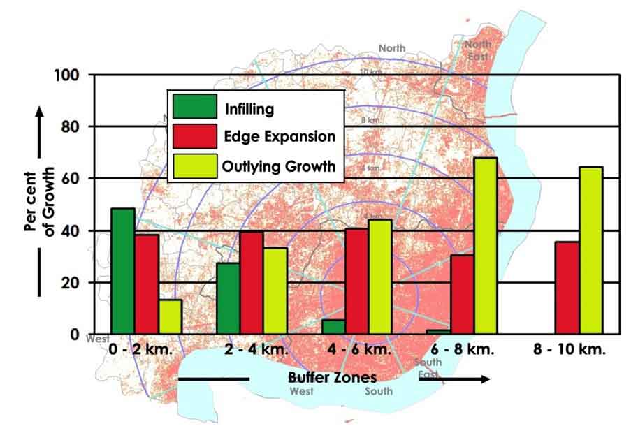
From Figure 7a, nearly 50% of urban growth in 2km buffer zone has identified as infilling type during 1996-2006 which was decreased sharply up to 8km buffer zone. No infilling has been found in 8-10km buffer. Edge expansion growth shows a steady growth along different buffer zones at an average of 36.87% to total growth. The outlying growth pattern was accounted for only 13.25% within 2km buffer but sharply increase along different buffer zone (Table 6). 6-8km and 8-10km buffer zone shows a spontaneous growth which implies a huge migration of rural population in the peri-urban portion of HMC. To study the pattern of such urban-rural gradient, directional analysis of growth pattern would be more helpful to throw light gradient driver variables, e.g. a) distance to major roads, b) distance from schools, c) distance to growth nodes, d) distance to urban civic amenities, etc.
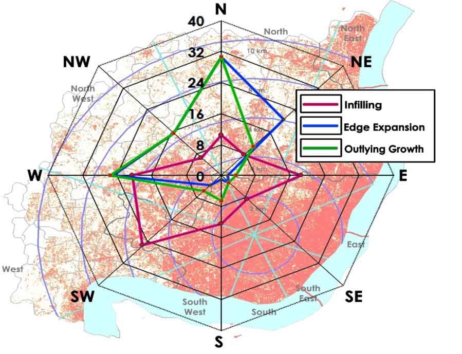
To comprehend the changed behaviour of growth types in urban setting with respect to directions from the urban core, eight directions have been created to identify the growth types (Figure 7b). During the study period (i.e. 1996-2016), infilling growth has been observed more than 20% in Southwest and West directions. East zone also accounts 18.5% of growth which was basically within the limit of HMC boundary as river Ganges make the eastern limit of HMC. Other five directions have not accounted for any significant growth in respect of infilling pattern. Edge expansion has not been found pointedly in North, Northeast, West and Northwest direction (Table 7). North, Northeast, Northwest directions lie within Bally municipality and HMC which attract such kind of growth pattern. Outlying growth also shows the same pattern of urban growth following the edge expansion type. From the directional analysis, it is very clear that the emergence of census towns (CT’s) have to make a contribution for such kind of outlying growth in the above-mentioned direction. Maximum outlying growth in the urban built-up area has been found in North and West direction at 30.5% and 25.5%, respectively.
Table 7. Urban growth types in different directions
|
Typologies of urban growth (%)
|
Directions
|
|
N
|
NE
|
E
|
SE
|
S
|
SW
|
W
|
NW
|
|
Infilling
|
10.50
|
7.50
|
18.50
|
8.50
|
12.50
|
25.50
|
20.50
|
6.50
|
|
Edge expansion
|
30.50
|
20.50
|
1.50
|
2.50
|
1.00
|
3.50
|
25.00
|
15.50
|
|
Outlying growth
|
30.50
|
10.50
|
3.50
|
2.50
|
6.50
|
5.50
|
25.50
|
15.50
|
5.3 Spatiotemporal Growth Pattern using Spatial Metrics
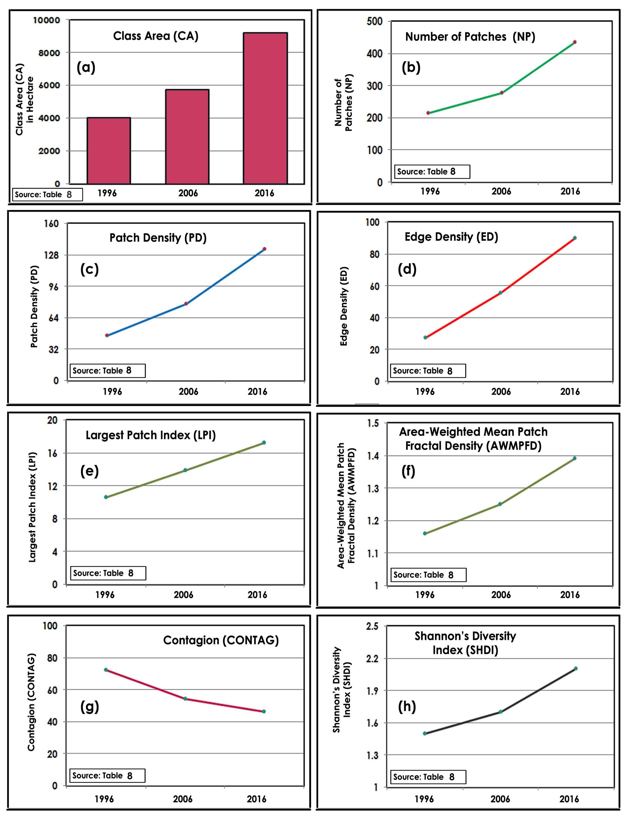
Spatial metrics is a very powerful tool to describe urban built-up quantitatively and compare the results using multi-date thematic maps. Eight often used spatial metrics have been selected on the basis of literature reviewed for the synoptic analysis of built-up dynamics over the space of HMC and its surroundings during 1996-2016 (Table 8, 9 and 10).
Table 8. Urban spatial metrics during 1996 - 2016
|
Temporal span
|
Urban spatial metrics
|
|
CA
|
NP
|
PD
|
ED
|
LPI
|
AWMPFD
|
CONTAG
|
SHDI
|
|
1996
|
4025
|
215
|
46
|
27.5
|
10.6
|
1.16
|
72.38
|
1.5
|
|
2006
|
5748
|
278
|
78
|
55.5
|
13.9
|
1.25
|
54.29
|
1.7
|
|
2016
|
9189
|
435
|
134
|
89.7
|
17.2
|
1.39
|
46.25
|
2.1
|
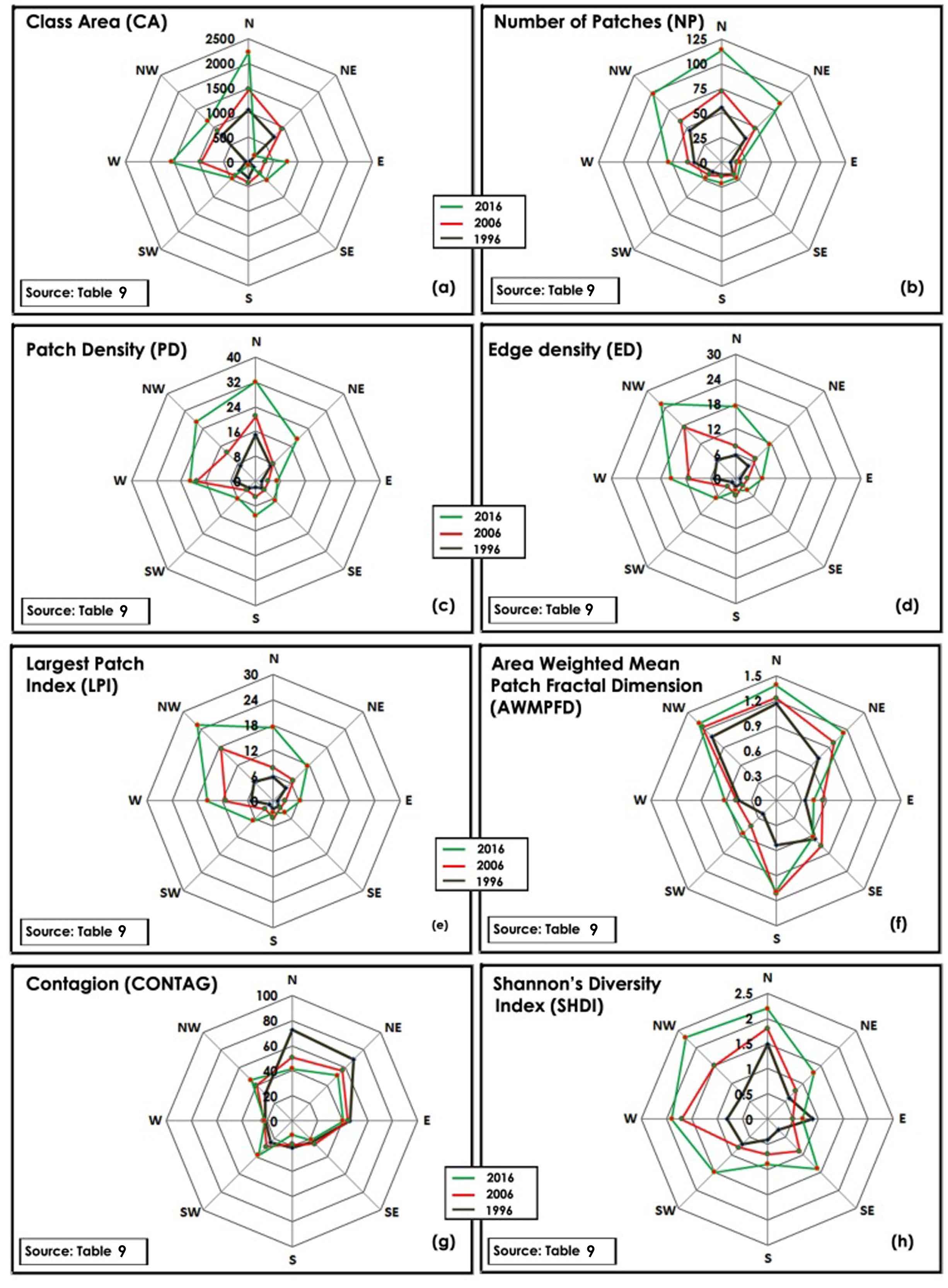
Table 9: Class and landscape level spatial metrics along different directions during 1996-2016
|
Directions
|
CA
|
NP
|
PD
|
ED
|
|
1996
|
2006
|
2016
|
1996
|
2006
|
2016
|
1996
|
2006
|
2016
|
1996
|
2006
|
2016
|
|
N
|
1065
|
1467
|
2234
|
56
|
72
|
114
|
15
|
21
|
32
|
5.6
|
7.9
|
17.4
|
|
NE
|
725
|
954
|
178
|
34
|
48
|
84
|
7
|
8
|
19
|
4.3
|
6.8
|
11.5
|
|
E
|
22
|
339
|
785
|
9
|
15
|
19
|
2
|
4
|
7
|
1.1
|
2.8
|
6.4
|
|
SE
|
138
|
324
|
525
|
17
|
18
|
22
|
3
|
4
|
9
|
1.7
|
2.4
|
3.9
|
|
S
|
325
|
422
|
67
|
12
|
14
|
21
|
2
|
5
|
11
|
1.9
|
4.1
|
2.8
|
|
SW
|
255
|
392
|
465
|
13
|
18
|
23
|
3
|
4
|
8
|
1.2
|
2.7
|
6.7
|
|
W
|
53
|
965
|
1565
|
28
|
34
|
54
|
7
|
19
|
21
|
5.2
|
11.3
|
15.6
|
|
NW
|
767
|
885
|
1165
|
46
|
59
|
98
|
7
|
13
|
27
|
6.5
|
17.5
|
25.4
|
| |
LPI
|
AWMPFD
|
CONTAG
|
SHDI
|
|
N
|
10.6
|
13.9
|
14.7
|
1.16
|
1.23
|
1.39
|
72.38
|
50.55
|
41.65
|
1.5
|
1.8
|
2.2
|
|
NE
|
7.3
|
4.2
|
3.9
|
0.72
|
0.98
|
1.15
|
68.98
|
56.87
|
50.98
|
0.6
|
0.8
|
1.3
|
|
E
|
1.5
|
2.4
|
2.7
|
0.35
|
0.56
|
0.45
|
45.67
|
44.32
|
40.35
|
0.9
|
0.5
|
0.7
|
|
SE
|
2.3
|
2.6
|
2.1
|
0.65
|
0.77
|
0.62
|
23.45
|
25.67
|
21.23
|
0.3
|
0.9
|
1.4
|
|
S
|
4.3
|
3.8
|
2.8
|
0.54
|
1.12
|
1.09
|
21.67
|
18.76
|
11.23
|
0.4
|
0.7
|
0.9
|
|
SW
|
2.9
|
3.2
|
4.4
|
0.23
|
0.43
|
0.56
|
23.67
|
28.85
|
38.29
|
0.7
|
0.8
|
1.5
|
|
W
|
3.2
|
4.6
|
7.9
|
0.45
|
0.48
|
0.62
|
21.34
|
22.56
|
21.85
|
0.8
|
1.7
|
1.9
|
|
NW
|
5.7
|
11.7
|
17.2
|
1.09
|
1.25
|
1.31
|
30.56
|
40.29
|
46.25
|
0.7
|
1.5
|
2.3
|
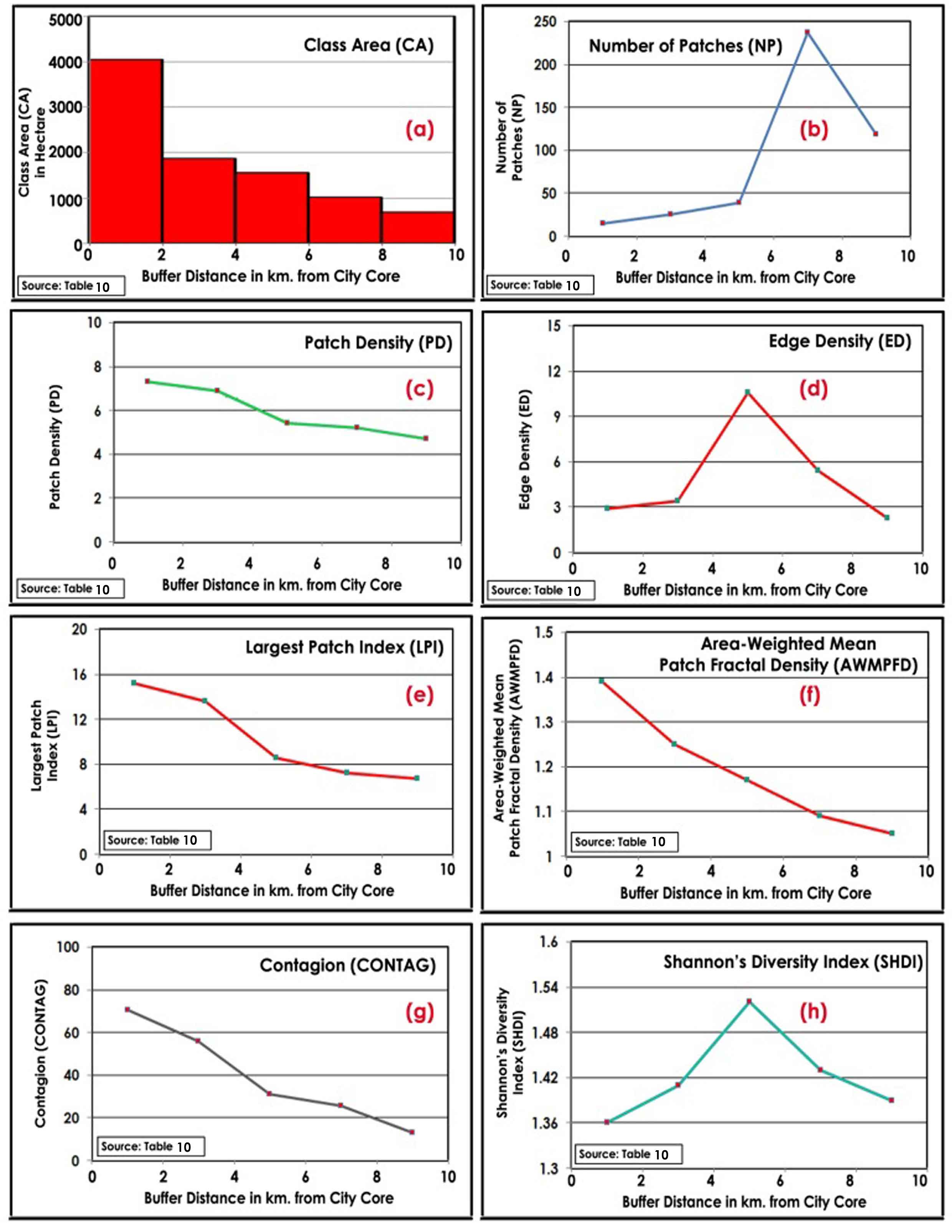
Table 10. Urban spatial metrics along different buffer zones during 1996 - 2016
|
Spatial metrics
|
Buffer zones
|
|
Up to 2km.
|
2-4km.
|
4-6km.
|
6-8km.
|
8-10km.
|
|
CA
|
4050
|
1870
|
1560
|
1020
|
691
|
|
NP
|
15
|
25
|
39
|
237
|
119
|
|
PD
|
7.3
|
6.9
|
5.4
|
5.2
|
4.7
|
|
ED
|
2.9
|
3.4
|
10.6
|
5.4
|
2.3
|
|
LPI
|
15.2
|
13.6
|
8.6
|
7.2
|
6.7
|
|
AWMPFD
|
1.39
|
1.25
|
1.17
|
1.09
|
1.05
|
|
CONTAG
|
70.4
|
55.7
|
30.9
|
25.6
|
13.2
|
|
SHDI
|
1.36
|
1.41
|
1.52
|
1.43
|
1.39
|
5.3.1 Class Area (CA)
Table 9 shows the result of class area (CA) has developed from 4025 hectares in 1996 to 5748 hectares in 2006 and to 9189 in 2016 (Figure 8a). In the second phase of the study period (i.e. 2006-2016) urban built-up has been estimated in highest rate which was nearly 60% (59.86 %) within 10 years. This specifies much speedy urban growth has been taking place during 2006-2016 in respect of 1996-2006. Growth of class area (CA) mostly found in the North, Northeast, west and Southwest directions during the last phase (Figure 9a). If the urban gradient is considered, within 2 and 8km buffer, class area (CA) has concentrated nearly 48%. Within 2-4 and 4-6km buffer most census towns (CTs) has emerged during 2001-2011 census periods which make an important characteristic to such kind of spatial metric (Figure 10a).
5.3.2 Number of Patches (NP)
The upsurge of number patches (NP) in HMC and its surrounding urban setting indicate rapid growth of urban built-up and the level of fragmentation in the built-up environment throughout the study period in different directions. The higher degree of NP shows the landscape fragmentation and lower values indicate the compact growth in the study region. Though during the study period mixed and split pattern urban growth process has taken place, and the substantial transformation has been perceived during 2006-2016 (Figure 8b). However bi-modal peak has been detected in North and Northwest directions (Figure 9b). In the case of NP analysis done through the urban gradient, the values increased very sharply as buffer distance increases. The significant inclination of the curve (Figure 10b) has been observed with 6-8km buffer which shows a clear indication of the growth of census towns (CTs) following outlying growth pattern. Patches at the city core of HMC tried to combine into a single clumped principal patch but the fragmentation is clear on the outer gradient.
5.3.3 Patch Density (PD)
Fragmentation category has been studied by applying another indication, i.e. patch density (PD). Increasing nature in built-up land use class shows the higher PD which is corroborated with fragmentation in an urban landscape setting (Figure 8c). During the second phase of the study, it has been observed that as the patch density increase sharply in North, Northeast and Northwestern direction where class area makes a high positive growth. This phenomenon has been detected through the gradient of two graphs (Figure 9c). On the other hand, decreasing nature of patch densities in East, Southeast, Southwest and South indicate some patches located in close immediacy to the city core following consistent urban fabric. The consequence has also been obvious with the growing LPI and signifies the arrangement amongst the urban spatial metrics (Figure 10c).
5.3.4 Edge Density (ED)
Another indicator to study the expansion of urban built-up area is the reckoning of edge density (ED). It is an indicator of the edge of the urban patches. As the land fragmentation increases the edge density increases simultaneously in a proportionate manner. During the study period (1996-2016) edge density has increased up to 89.7 in 2016 from 27.5 in 1996 which mark an imprint that the landscape fragmentation is increasing during the study period (Figure 8d). Most edge density has been found prominent within 4-6km buffer with 10.6 values (Table 9). If the urban-rural direction is concerned, Northwest (25.4), North (17.4) and West (15.4) making major attribution to the edge density showing the high spontaneous growth or outlying pattern of urban growth type (Figure 9d).
5.3.5 Largest Patch Index (LPI)
Largest Patch Index (LPI) has been figured out to epitomize the proportion of the landscape that comprises the prevalent patch in the study area. Intrinsically, the foremost or largest patch in the landscape backing to be the urban core has mature over the study period within 2km buffer. As the buffer distance has increased, the value of LPI shown a decreasing trend which proves the infilling and edge expansion nature of urban growth in 0-4km buffer from city core. This gradual expansion of the urban core towards North and Northeast might have change HMC into an agglomeration growth with Bally municipality located in the North in future (Figure 9e). Declining trends of LPI in the outer buffer (Figure 10e) in different directions express the expansion of urban built-up in scattering and fragmented manner.
5.3.6 Area-Weighted Mean Patch Fractal Density (AWMPFD)
Urban patch shape complexity has been shown using Area-Weighted Mean Patch Fractal Density (AWMPFD) which actually shows how the patch perimeter increases in patch area within the study period. In 1996, AWMPFD was 1.16 which designates a unit increase in patch area, up to 16% and by 39% perimeter increase in 2016. During 1996-2016, increasing nature of AWMPFD might be due to fragmented growth and emergence of new towns in and around HMC (Figure 8f). In East, South and Southeast directions value of AWMPFD has decreased during 1996-2016 implies the stabilized growth and connect up of the built-up area around the city core mark a simple and steady urban form (Figure 9f). When looking at the highest value of AWMPFD (1.39 in North direction), it implies that during the study period, the geometry and morphology of urban patches receiving more complexity (Figure 10f).
5.3.7 Contagion (CONTAG)
CONTAG specifies the level of built-up fragmentation with the reducing value while an increase measures the degree of the clumpiness of built-up patches. From the Table 9 and Table 10, it has been observed that the value of CONTAG is decreasing in the buffer area (4-10km) but has become low towards city (Figure 10g) core which implies the clumpiness towards the urban core. In North, Northeast, South and Southeast the values of CONTAG has been found an increasing trends whereas in the outer buffer of West, Northwest and Southwest, CONTAG has been found in low (Figure 9g) values indicating fragmented growth pattern.
5.3. Shannon’s Diversity Index (SHDI)
The diversity of landscape characterized by Shannon’s Diversity Index (SHDI) implies varieties in landscape types, shape and number of patches with their inlay pattern. A ridge of SHDI is clearly found within 4-8km buffer zone (1.52 with maximum value) and fallen towards 10km buffer zone (Figure 10h). SHDI increased in different directions along with patch density nearly in a proportionate way which shows the complexity of composition and configuration of urban built-up landscape. The decreasing number of SHDI implies the built-up characteristics were more similar with the neighboring patches under the condition of urban growth and hence the landscape character became simple. All the results from Table 9 shows that the urban fragmentation mainly occurring in three directions among the eight directions within the study periods.


 ,
Sanjit Kundu 2
,
Sanjit Kundu 2
 ,
Subrata Haldar 2
,
Subrata Haldar 2