Keywords

Damanganga Basin , Flood Frequency , Gumbel Extreme Value type I , Log Pearson Type III

1 . INTRODUCTION

An analysis of flood magnitude and frequency is a crucial aspect in the studies of hydro-meteorology, flood geomorphology, flood hydrology, and civil engineering (Makkonen and Tikanmäki, 2019). Therefore, it is essential to select an appropriate probability distribution method for the investigation of magnitude and frequency of floods while evaluating the design flood with return period before the construction dams and bridges (Chow et al., 1988; Hosking and Wallis, 1997). A design flood is the estimated peak discharge at a given site on a river adopted for the design of a structure (Prasad and Subramanya, 1986). However, there is not a single universally recognized magnitude-frequency probability distribution method (Law and Tasker, 2003). As a result, choice of the appropriate magnitude-frequency probability distribution method from numerous methods (Gumbel Extreme Value type I (GEVI), Log Pearson type III (LP-III), Generalized Extreme Value (GEV), Log-Normal (LN), etc.)) is crucial and challenging task of hydrologist and civil engineers.

The U.S. Water Resources Council (USWRC, 1967; 1976; 1981) had suggested that LP-III is the best method for the analysis of magnitude-frequency of floods. However, the GEVI probability distribution method has been applied and recommended by several scholars for predicting flood magnitude and its return period (Gumbel, 1958; Todorovic, 1978; Watt et al., 1989). Besides, numerous studies also focused on the application of the LP-III technique for probability estimation of the magnitude and recurrence interval in the different hydroclimatic environment (Matalas and Wallis, 1973; Phien and Jivajirajah, 1984; Griffis and Stendinger, 2009; Myronidis and Ivanova, 2020). Further, Srikanthan and McMahon (1981) applied the LP-III distribution to the annual maximum discharges of the river in Australia. 

According to Merz and Blöschl (2008b) and Elleder (2010) accuracy of a hydraulic probability distribution technique is based on the accuracy and length of the available data. However, a continuous Annual Maximum Series (AMS) data of 30 years can be an acceptable period for Flood Frequency Analysis (FFA) (Garde, 1998). In recent times, numerous researchers have applied GEVI and LP-III probability distribution techniques for the FFA of Indian rivers (Jha and Bairagya, 2011; Patil, 2017; Hire and Patil, 2018; Pawar and Hire, 2019; Pawar, 2019; Bhat et al., 2019; Pawar et al., 2020; Samantaray and Sahoo, 2020; Sheikh et al., 2020). Nevertheless, identification of the best-fit probability distribution method is the prime concern in the FFA by applying tests of goodness-of-fit (GoF) (Haddad and Rahman, 2011). As the Damanganga Basin receives heavy spells of rainfall throughout the southwest monsoon season that causes floods in the basin, an attempt has been made to compare and select the best-fit probability distribution for magnitude-frequency analysis between GEVI and LP-III by using GoF tests. Accordingly, discharges for various recurrence intervals (Q₂, Q₅, Q₁₀, Q₂₅, Q₅₀, Q₁₀₀, and Q₂₀₀ years) were estimated and the return period for recorded high magnitude discharges at every site in the Damanganga Basin during the gauge period was determined by the best-fit flood frequency probability distribution techniques.

2 . STUDY AREA

The Damanganga River is one of the inter-state west-flowing rivers in western India. It has source at an elevation of 950 m in the Western Ghat near Ambegaon in Dindori tehsil of the Nashik district (Figure 1). The river flows for a length of 140 km in the west and joins the Arabian Sea (near Daman) in the south of the Gujarat State. The Damanganga Basin extends over parts of Maharashtra, Gujarat, Union Territory of Dadra and Nagar Haveli, and Daman. The total area of the basin is 2300 km² comprises 59% area of the Nashik (Maharashtra), 21% area of the Valsad (Gujarat), and 20% area of the Union Territories of the Dadara and Nagar Haveli as well as Daman. The Wagh River is the main tributary of the Damanganga River that flows for a length of 54 km and joins the Damanganga River from left-bank near Malungi village of the Valsad district of Gujarat in the South. The geology of the Damanganga Basin comprised rock of the Deccan Trap Basalt (Mahoney et al., 2002). The Annual Average Rainfall (AAR) of the basin is 2261 mm and about 94% of rainfall occurs during the monsoon season (June-September) (Figure 2). Moreover, the basin receives heavy to very heavy rain spells during the southwest monsoon season (June-September) under the influence of Monsoon Depressions (MD) developing either over the Bay of Bengal (BoB) and adjoining land or the Arabian Sea.

Figure 1. Study area: Damanganga Basin with discharge gauging sites

Figure 2. Monthly average rainfall of the Damanganga Basin

3 . MATERIALS AND METHODS

3.1 Database

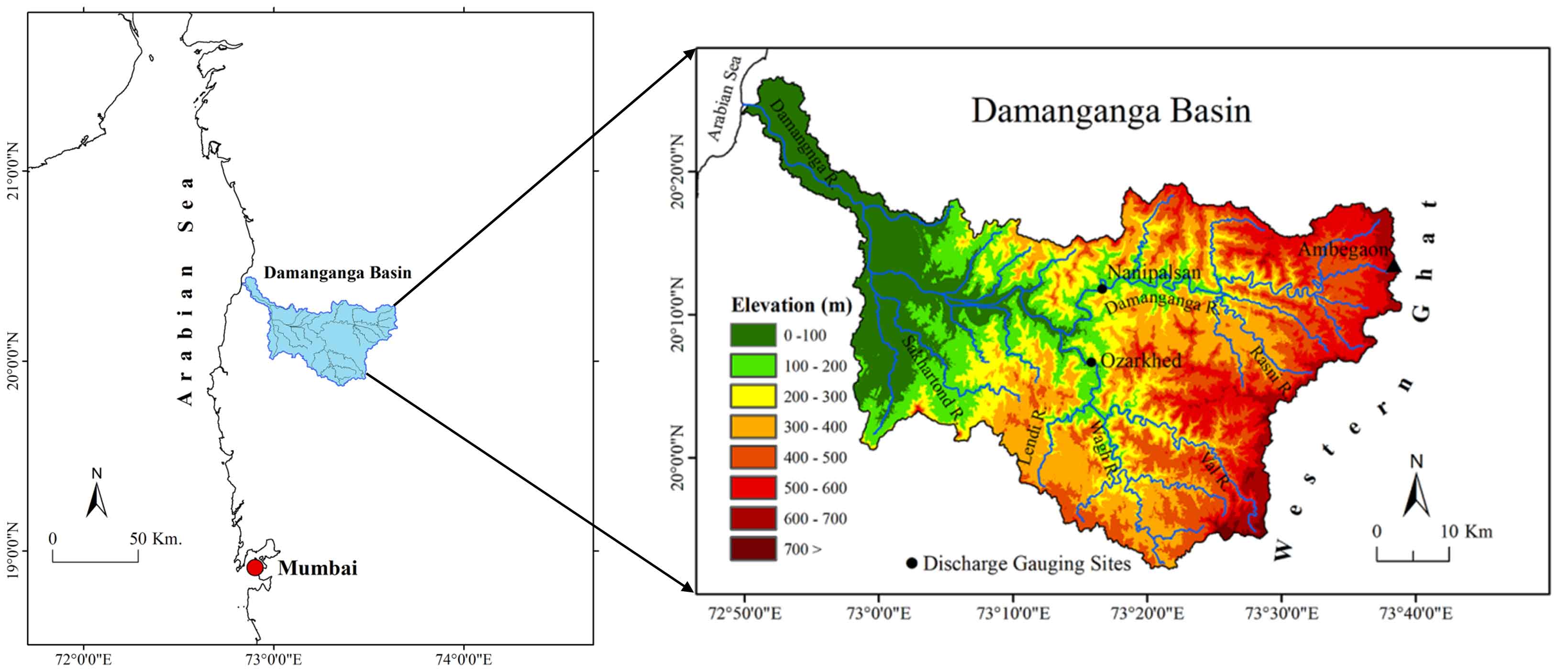
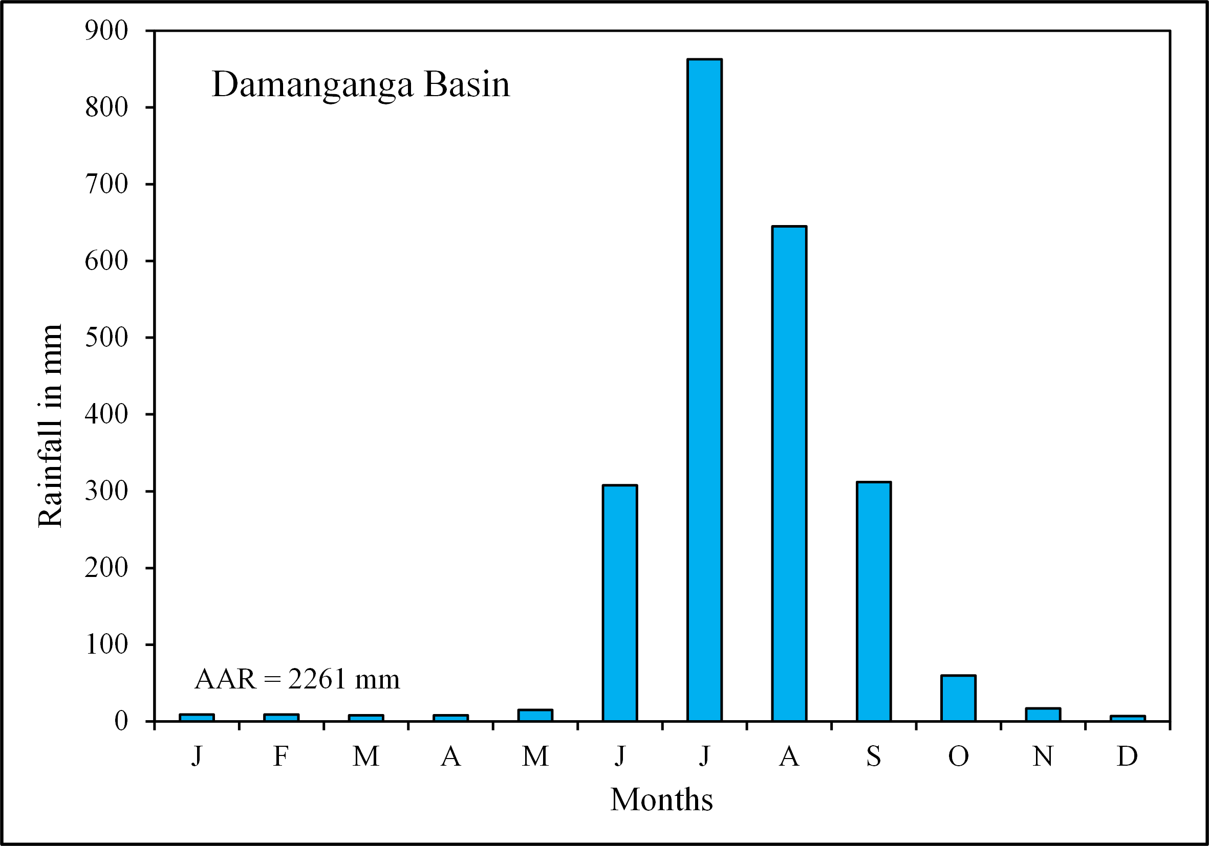
Flood Frequency Analysis (FFA) of the Damanganga Basin was carried out by using AMS data. Accordingly, AMS data were procured from the water year book 2017-18 published by Central Water Commission (CWC), Gandhinagar (Gujarat). The data were available for the Damanganga River at Nanipalsan and the Wagh River at Ozarkhed gauging sites located in the Damanganga Basin (Figure 1). The record length for both sites is 27 years from 1991 to 2017. Additionally, rainfall data of the Damanganga Basin were procured from the India Meteorological Department (IMD), Pune, to comprehend the mean rainfall characteristics of the Damanganga Basin. Table 1 specifies hydrological and geomorphological characteristics of the Damanganga Basin at sites under the study.

3.2 Methodology

The flood discharge characteristics of the Damanganga Basin were derived by applying elementary quantitative techniques (mean, standard deviation (σ), coefficient of variation (C_v), and coefficient of skewness (C_s)) to AMS data. Further, the best-fit probability distribution at both sites (Nanipalsan and Ozarkhed) was selected by using the Kolmogorov-Smirnov (KS) test and Anderson Darling (AD) test of GoF. The discharges for various recurrence intervals (Q₂, Q₅, Q₁₀, Q₂₅, Q₅₀, Q₁₀₀, and Q₂₀₀ years) were predicted based on GEVI (Gumbel 1941, 1958) and LP-III (Pearson, 1916) probability distributions. Besides, the return periods for mean annual peak flows (Q_m), large floods (All floods that exceed the mean plus one standard deviation (Q_lf)), and observed peak discharge on record during gauge period (Q_max) were calculated by using GEVI and LP-III probability distribution (Hire, 2000).

3.2.1 Gumbel Extreme Value type I (GEVI) Model

An identification of the best-fit flood frequency probability distribution at every site in the Damanganga Basin is the prime focus of this research. Therefore, the widely applied probability technique of GEVI was used for the estimation of recurrence interval of the flood and discharges for various recurrence interval by applying equation (1), (2) and (3):

\(\overline{Q} = { \sum Q \over n}\)                         (1)

\(\sigma {Q} = \sqrt{\frac{\sum(Q-\overline{Q})^2}{n-1}}\)             (2)

\(Q_T = \overline{Q} + (K_{(T)}*\sigma{Q})\)     (3)

where Q_T is a discharge of given return period; \(\overline{Q}\)  is a mean annual peak discharge; n is the number of years of records; σQ is a standard deviation of AMS and K_(T) is a frequency factor which is the function of the return period T. Consequently, K_(T) values were obtained from the book entitled “Hydrology in Practice” by Shaw (1994).

The return periods were calculated for Q_m, Q_lf, and Q_max at each site using equations (4), (5), (6), and (7):

\(F(X)=e[-e^{-b(x-a)} ) ]\)          (4)

where, F(X) is the probability of an annual maximum Q ≤ X and a and b are two parameters related to the moments of the population of Q values.; e is the exponent. The parameters ‘a’ and ‘b’ were determined by using equations (5) and (6):

\(b = { \pi \over {\sigma Q \sqrt{6} }}\)                 (5)

\(a =\overline{Q} - { y \over b}\)               (6)

(γ = 0.5772)               

Lastly, the recurrence interval for desired discharges (Qm, Qlf, and Qmax) was designed using equation (7):

\(T = {\frac{1}{1-F(X)}}\)             (7)

where, F(X) is the probability of an annual maximum obtained using equation (4).

3.2.2 Log Pearson Type III (LP-III)

The LP-III probability distribution was applied by Foster (1924) for estimating flood discharges and return period. Bedient and Huber (1989) specified that when log values of the AMS data are used then it is referred to as the LP-III probability distribution. In this analysis, design floods for Q₂, Q₅, Q₁₀, Q₂₅, Q₅₀, Q₁₀₀, and Q₂₀₀ year return period were also estimated by LP-III probability distribution with the help of the following equations:

\(\overline{LogQ} = {\frac {\sum logQ}{n}}\)                               (8)

\(\sigma {LogQ} = \sqrt{\frac{\sum(logQ-\overline{logQ})^2}{n-1}}\)               (9)

\(C_s = {n* \sum (logQ - \overline {logQ}^3) \over (n-1)*(n-2)*({\sigma}logQ)^3}\)                  (10)

\(logQ_T= {\overline{logQ}} ̅+( K_{(T)}*σ log Q ) \)     (11)

\(Q_T=Antilog(logQ_T ) \)                     (12)

where, logQ_T is the base 10 logarithms of the discharge of desired return period; \(\overline{logQ}\) is a mean of the logarithms of AMS; σ_logQ is a standard deviation of the logarithms of AMS and K_(T) is a frequency factor of the return period (T). The K_(T) value is based on the skewness coefficient of the logarithms of AMS data. The K_(T) values were acquired from Hydrology book (Raghunath, 2006).

3.2.3 Plotting Position and Frequency Curves

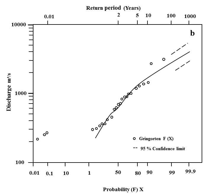
In view of Cunnane (1978) and Shaw (1988), the Gringorten formula for plotting position and frequency curve is the best-fit because the outliers fall into line better than other plotting positions. Therefore, F(X) values were computed by applying the subsequent equations (Gringorten, 1963):

\(P(X) = {\frac{r-0.44}{N+0.12}}\)            (13)

\(F(X) = 1-P(X) \)       (14)

where, r is flood magnitude ranks (from largest to smallest); N is the number of years of records; P(X) is the probability of exceedance. The Gumbel probability graph paper and Log-probability graph paper were used to plot Flood Frequency Curves (FFC). The FFC were derived based on results of the GoF at a site. The 95% confidence limit was placed on FFC. A method proposed by Beard (1975) was applied to form the reliability band of the confidence limit.

3.2.4 Goodness-of-Fit (GoF)

The tests of GoF are indispensable to select the best-fit distribution amongst several probability distributions (Millington et al., 2011). Therefore, the most extensively applied KS and AD test were used and results were obtained using the Easyfit software.

4 . RESULTS AND DISCUSSIONS

4.1 Annual Maximum Series (AMS) Analysis

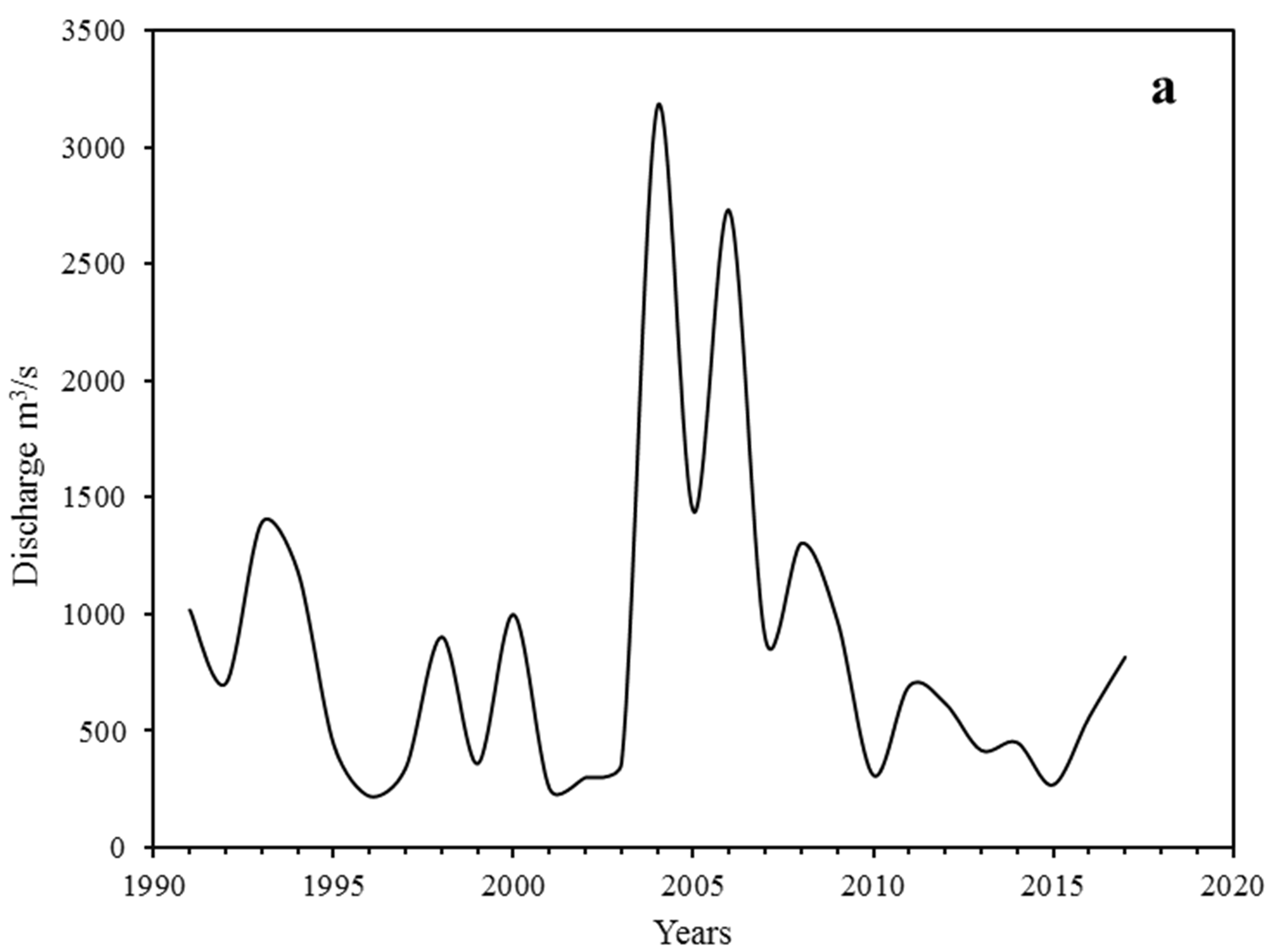
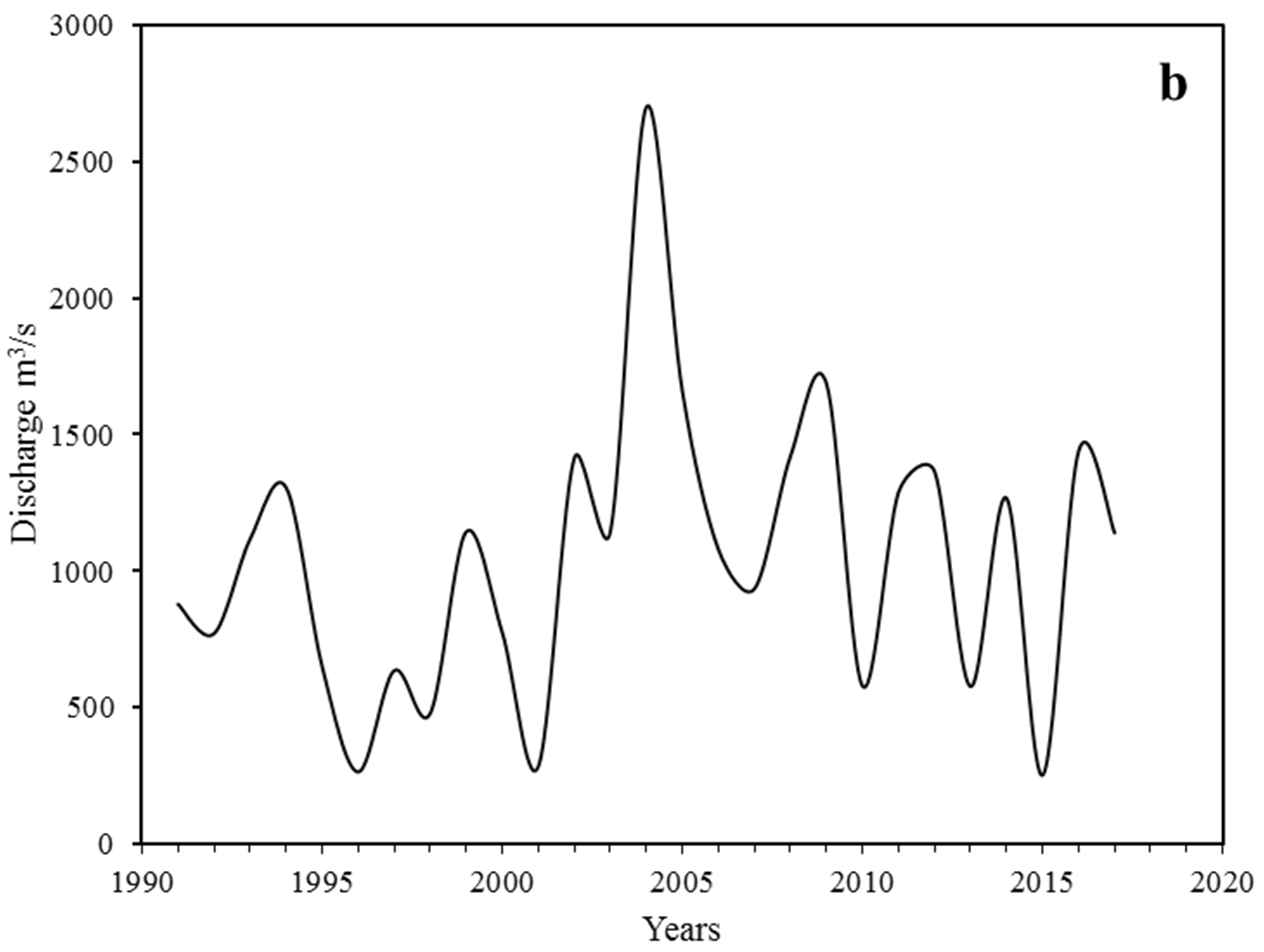
The statistical analysis reveals that the coefficient of variation (C_v) ranged between is 0.83 (Nanipalsan) and 0.51 (Ozarkhed). The highest value of the coefficient of skewness (2.07) of the Nanipalsan site specifies occurrence of the high-magnitude floods during the gauge period in the Damanganga Basin. Further, Q_max/Q_m ratio indicates that Q_max (the largest floods during the gauge period) recorded at both sites in the Damanganga Basin was about three-to-four times higher than Q_m (mean annual flows) (Table 2). Figure 3a and 3b show a year-to-year variation with one or two large flood peaks throughout the gauge period in the Damanganga Basin.

Figure 3a. Annual maximum series: Damanganga River at Nanipalsan

Figure 3b. Annual maximum series: Wagh River at Ozarkhed

4.2 Goodness-of-Fit Analysis (GoF)

The prime objective of the FFA of the Damanganga Basin is an identification of the best-fit probability distribution at sites under investigation. Accordingly, KS and AD tests of GoF were used to AMS in Easy-fit software and results were acquired by considering critical value at a 95% confidence level (α=0.05). The ranks were given to the probability values for GEVI and LP-III. Rank 1 shows best-fit distribution and ranks 2 specifies elimination of the probability distribution techniques at each site (Table 3). According to the KS and AD tests analysis, the results of acceptance and rejection were the same for both sites (Table 3). The comparative analysis of GEVI and LP-III indicates that LP-III is the best-fit probability distribution for sites (Nanipalsan and Ozarkhed) in the Damanganga Basin.

4.3 Estimation of Discharges for the Return Period

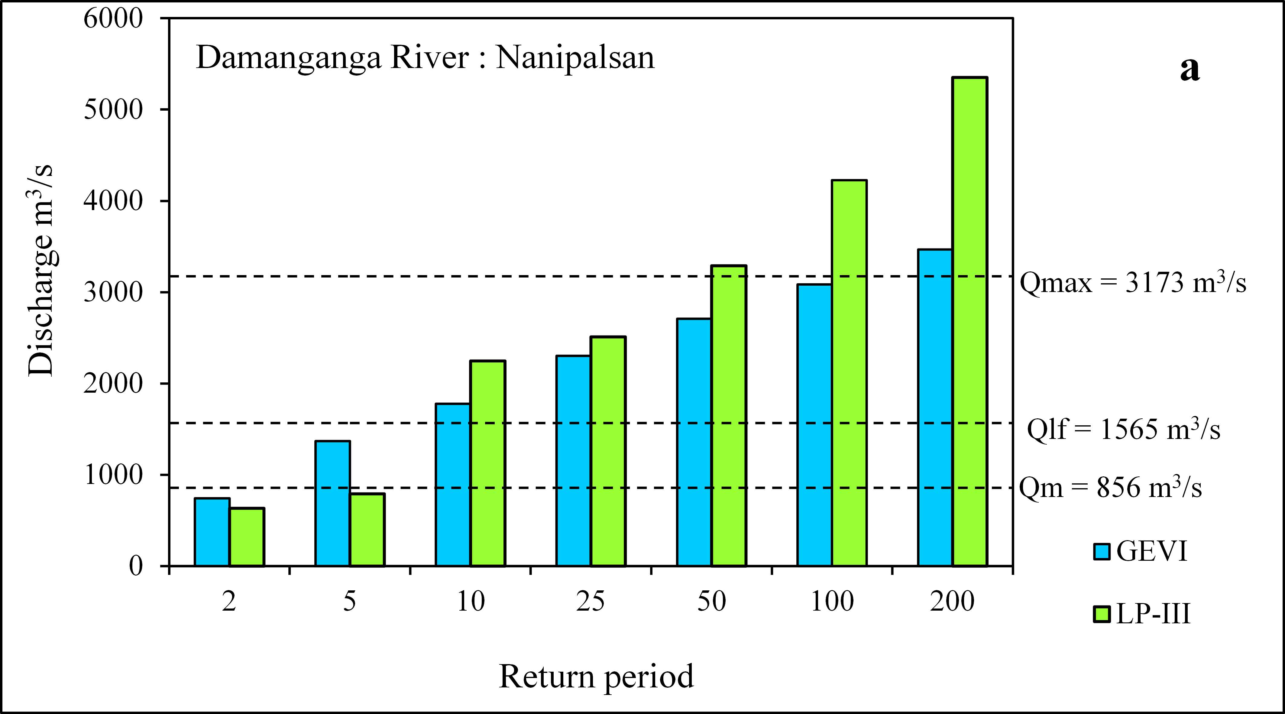
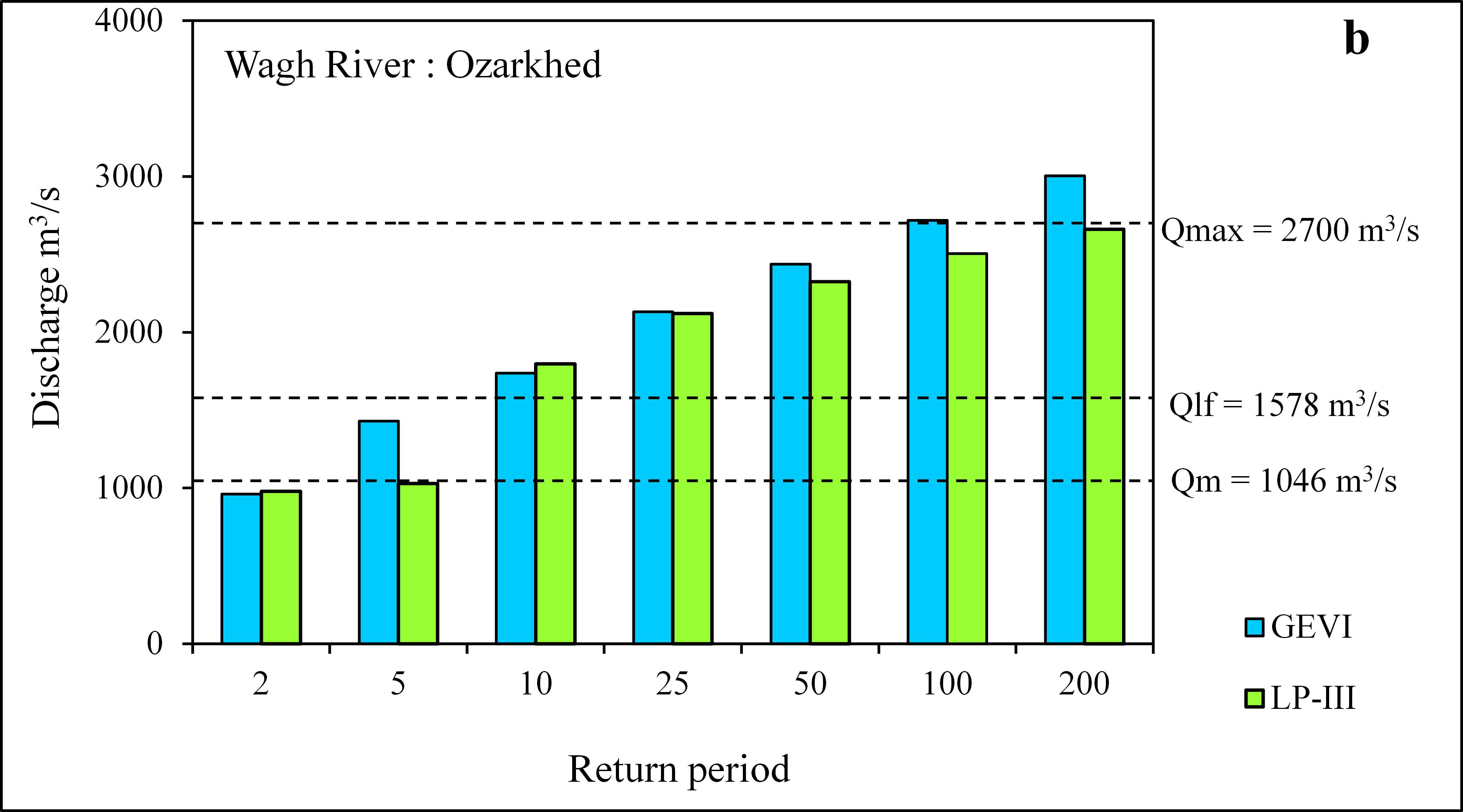
One of the purposes of the FFA is to predict discharges for various recurrence intervals. Accordingly, discharges were estimated for Q₂, Q₅, Q₁₀, Q₂₅, Q₅₀, Q₁₀₀, and Q₂₀₀ years return period by GEVI and LP-III probability distribution techniques, and results have been shown in (Table 4). The comparison of estimated discharges by GEVI and LP-III (Table 4) denotes that estimated discharge (3288 m³/s) by best-fit distribution (LP-III) for Q₅₀ recurrence interval at Nanipalsan is close to the observed Q_max (3173 m³/s) (Table 2; Table 4). In the case of the Ozarkhed site on the Wagh River, the estimated discharge of the Q₂₀₀ return period shows nearness with the observed Q_max (2700 m³/s). The peak discharge (Q_max = 3173 m³/s) on the Damanganga River (at Nanipalsan) was observed in the year 2004 (Table 2). Therefore, to estimate accurate discharges using the best-fit probability distribution for the flood studies and designing of the hydraulic structures is an integral part of the FFA (Chow et al., 1988; Hosking and Wallis, 1997). The Figure 4a and 4b show that the predicted discharges for different recurrence intervals are near the observed floods (Q_m, Q_lf, and Q_max) as per GEVI and LP-III probability distribution. Moreover, graphs (Figure 4a and 4b) show that predicted flows Q₂ return period are less than the average annual discharges (Q_m).

Figure 4a. Estimated discharge for different return period by GEVI and LP-III

Figure 4b. Estimated discharge for different return period by GEVI and LP-III

4.4 Estimation of the Return Period

According to Kale and Gupta (2010), the high magnitude floods that have recurrence interval of several decades are more catastrophic than that of the average annual flows (Q_m). Therefore, it is important to estimate the return period of the observed high magnitude floods during the gauge period. Accordingly, return periods for Q_m, Q_lf, and Q_max were predicted using GEVI and LP-III probability methods. The result of GEVI probability distribution shows that the return periods for Q_m, Q_lf (Q_m +1σ) for both sites (Nanipalsan and Ozarkhed) in the Damanganga Basin are 2.33 and 6.93 years respectively. However, the recurrence interval for Q_max ranged between 96 years (Ozarkhed) and 118 years (Nanipalsan) as per the GEVI (Table 5). The LP-III analysis indicates that the return period of Q_m is 7.42 year for Nanipalsan (Damanganga River), and 5.52 years for Ozarkhed (Wagh River). The return periods of the large flood (Qlf) obtained by the LP-III probability distribution for Damanganga River at Nanipalsan and Wagh River at Ozarkhed are 28.10 years and 23.09 years respectively. Moreover, the estimated return period by LP-III for Q_max at Nanipalsan (Damanganga River) and Ozarkhed (Wagh River) is 107 years and 146 years respectively (Table 5). The comparative study of GEVI and LP-III shows that the LP-III probability distribution is best-fitted for both the sites (Nanipalsan and Ozarkhed) and is appropriate to estimate design flood for constructions of hydraulic structures and disaster management in the Damanganga Basin.

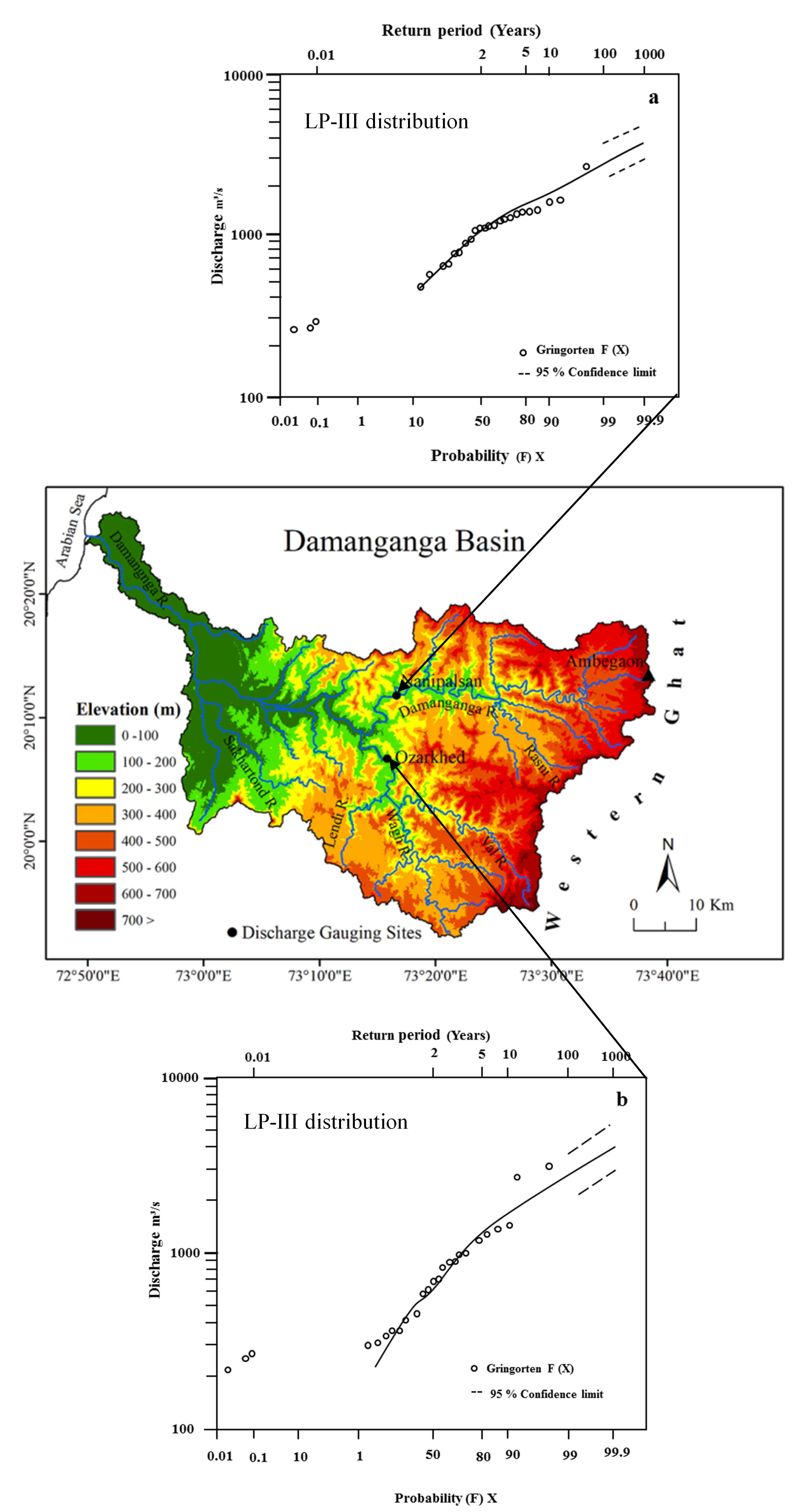
4.5 Flood Frequency Curve (FFC)

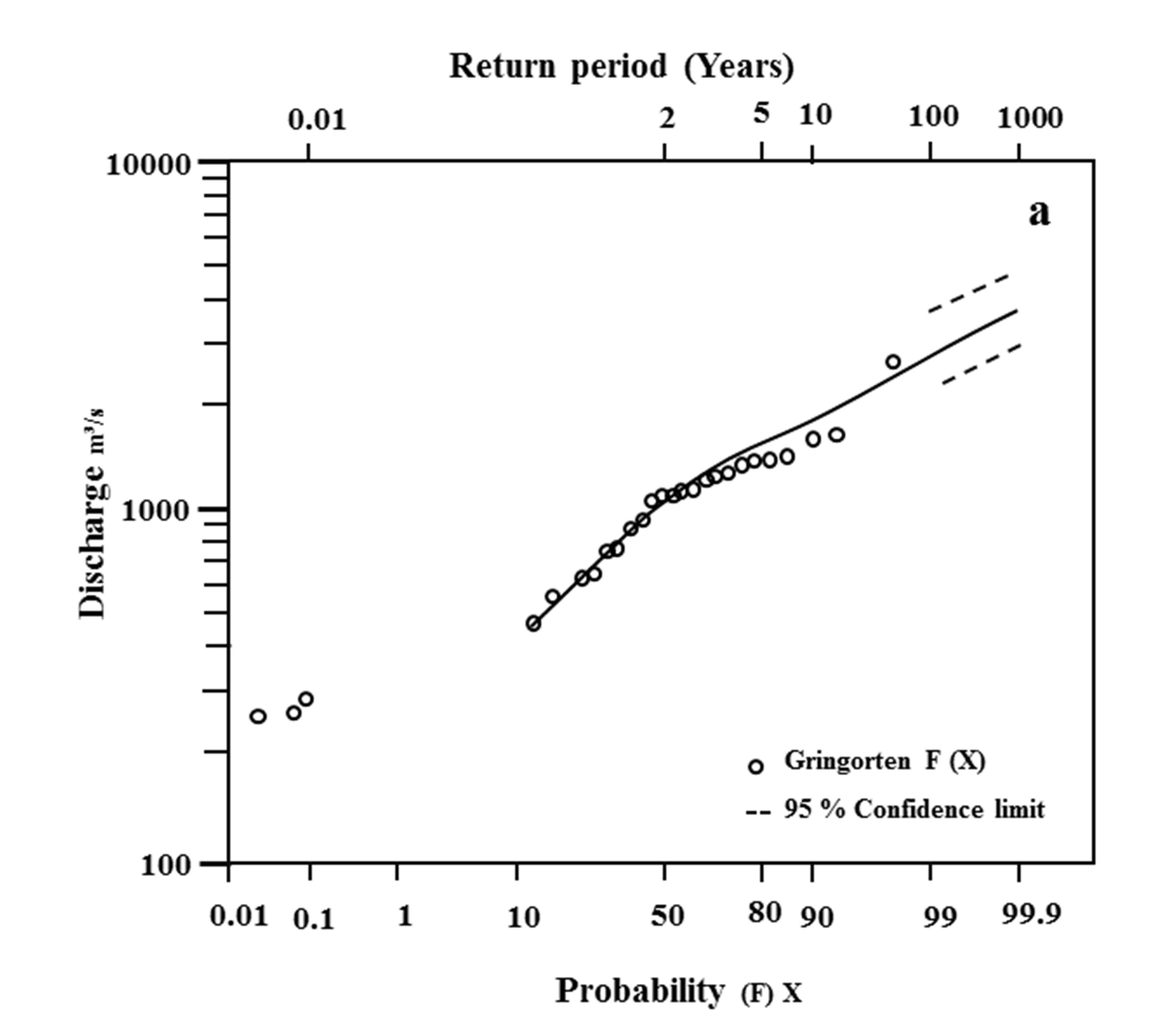
The FFC were obtained as per the results of the test of GoF for Nanipalsan and Ozarkhed. The LP-III probability distribution is best-fit for both the sites in the Damanganga Basin. Therefore, FFCs were obtained only for LP-III probability distribution by best-fit line to AMS data plotted on Log probability graph paper (Pawar et al., 2020). The FFC shows that the best-fit lines are fairly adjacent to most of the AMS data points and, therefore, can be reliably and conveniently used to obtain the return period for a specified magnitude and vice versa (Figure 5a and 5b).  Besides, to predict the future trend of the discharge, 95% confidence limit was calculated for each graph and shown by dotted lines. The FFC of Nanipalsan and Ozarkhed sites show a rising trend in the magnitude of discharges but within the confidence limits. The graphs indicate that the return periods of Q_max at Nanipalsan and Ozarkhed sites in the Damanganga Basin predicted by LP-III are likely to be relatively trustworthy and can be used for the designing of hydraulic structures (dams and bridges) on the Damanganga and Wagh Rivers. Consequently, the LP-III model is best-fitted for the flood frequency analysis of the Damanganga Basin.

Figure 5a. Flood frequency, annual maximum series, LP-III distribution: Damanganga River (Nanipalsan)

Figure 5b. Flood frequency, annual maximum series, LP-III distribution: Wagh River (Ozarkhed)

5 . CONCLUSIONS

Tables

Figures

Conflict of Interest

Acknowledgements

Abbreviations

References