Keywords

Geospatial analysis , GIS , Groundwater , Thematic Layers , AHP model

1 . INTRODUCTION

In the current times with the burgeoning need for groundwater is augmenting in drinking, domestic and agricultural activities has amplified significance of groundwater as sustainable water resource radically with its low pollution imprints and also acting as climate change buffer. Globally groundwater use has influenced ‘environmentally critical stream flow’ in more than 15% of streams, and could affect most of them by 2050 (de Graaf et al., 2019). Groundwater contributing around 34% of the total annual water supply is a vital and dynamic natural fresh water resource (Shekhar and Pandey, 2015) supporting bio-physical, ecological and human health environments. Significant population of India relies on groundwater sources for consumption (drinking and domestic purposes), with 90% of rural population and nearly 30% of urban populace resulting in over exploitation in some regions (Parthasarathy and Deka, 2019). India’s annual groundwater withdrawal rate is estimated to be 251 km³ (Gun, 2012). Groundwater caters to nearly 85% of rural, 65% of irrigation and 50% of urban drinking water/industrial needs in the India (India Water Portal, 2019). Water scarcity affects approximately 0.6 billion people in the country having high water stress caused by a lack of freshwater, with almost three-quarters of households lacking access to potable water (NITI Aayog, 2018) . India will become a water-stress zone by 2025, and then a water-scarce zone by 2050, unless stringent steps are taken (World Bank, 2005). However, its availability is limited because groundwater is mostly an ‘invisible resource’ on the earth’s surface as it is found in complex subsurface formations, with fluctuating signals of flow. Groundwater being a quintessential resource in both the developed and developing nations having varied hydro-meteorological regimes also caters to a large populace worldwide as around one-third population consumes groundwater for drinking purposes (Arkoprovo et al., 2012).

Globally groundwater has emerged as primary source with more than 65% of agricultural activities depending upon it as a source for irrigation (World Bank, 2012). Extreme levels of intensification with respect to groundwater development in certain regions of India lacking appropriate groundwater management regimes has resulted in its over-abstraction thus leading to a decreasing trend in groundwater levels (Srivastava et al., 2012; CGWB, 2016). The availability of groundwater estimated for India is 399 billion/m³ (MOWR, 2009). Consequently, there is a pressing requirement for mapping the areas having prospects of holding significant groundwater resources for sustainable use. Groundwater potential study includes the delineation and outlining of areas or expanses which have the markers of being prospective aquifers for the specified area. The aquifer productivity, though, relies on the geomorphology and topographical configurations prevalent in certain region with structural and lithological agents that directs the flow of groundwater, groundwater yielding zones and hydrogeological conditions. There should be an equilibrium mechanism in hydrogeological systems of piedmont and areas with mountainous terrain both at the regional and local scales which is largely directed by the flow regimes from the upstream areas to recharge the valley aquifers (Cremonesi et al., 2008). The specificity in the regions having relatively sparse vegetation and higher rate of gradient in slopes usually reflects the scarcity of water leading to a very low rate of groundwater discharge in the aquifers. Therefore, this demands an all-inclusive evaluation for groundwater assessment and potential analysis of the region.

Globally, numerous studies employing geological and hydrogeological studies have used range of conventional techniques for assessment of groundwater source regions ( Oh et al., 2011; Mohammadi-Behzad et al., 2018) and have taken the aid of geo-physical and reconnaissance (Edet and Okereke, 2002; Layade et al., 2017) techniques having highly drawn out, time-consuming, and expensive considerations. On the other hand remote sensing based approach using the multi-temporal spatial datasets has proved to be an effective mechanism in saving the time, reducing the cost components and is easier to approach with precise and detailed analysis of complex hydrogeological environments. GIS provides a less tedious approach for spatial data management and is a powerful tool not only for information analysis but also having the predictive abilities in complex decision environments. Moreover, RS and GIS based method is sufficient for precisely mapping and assessing of groundwater prospective regions.

Remote sensing and GIS technology has been considered as quintessential method for having the effective and reasoned managing of critical groundwater sources (Machiwal et al., 2011). Most of the literature reveals that satellite imagery (remote sensing) and GIS are largely employed in hydro-geomorphological investigations. Several researchers (Sreedevi et al., 2005; Sankar, 2002; Israil et al., 2006; Javed and Wani, 2009; Jia et al., 2011; Ozdemir, 2011; Rahmati et al., 2015; Thilagavathi et al., 2015; Malik et al., 2016; Naghibi et al., 2016; Zabihi et al., 2016; Ghorbani Nejad et al., 2017; Kumar et al., 2011; Halder et al., 2020) applied geospatial techniques in evaluating and representing the groundwater potential areas of occurrence in different regions. Although satellite imagery cannot directly detect groundwater due to its complex sub-surface environment, the features curated from such datasets (e.g., landforms and fractures) determine the influencing factors for predictive analysis for groundwater potentiality (Tiyip et al., 2002; Vittala et al., 2005; Jha and Peiffer, 2006; Adiat et al., 2012; Hammouri et al., 2012; Li et al., 2016).

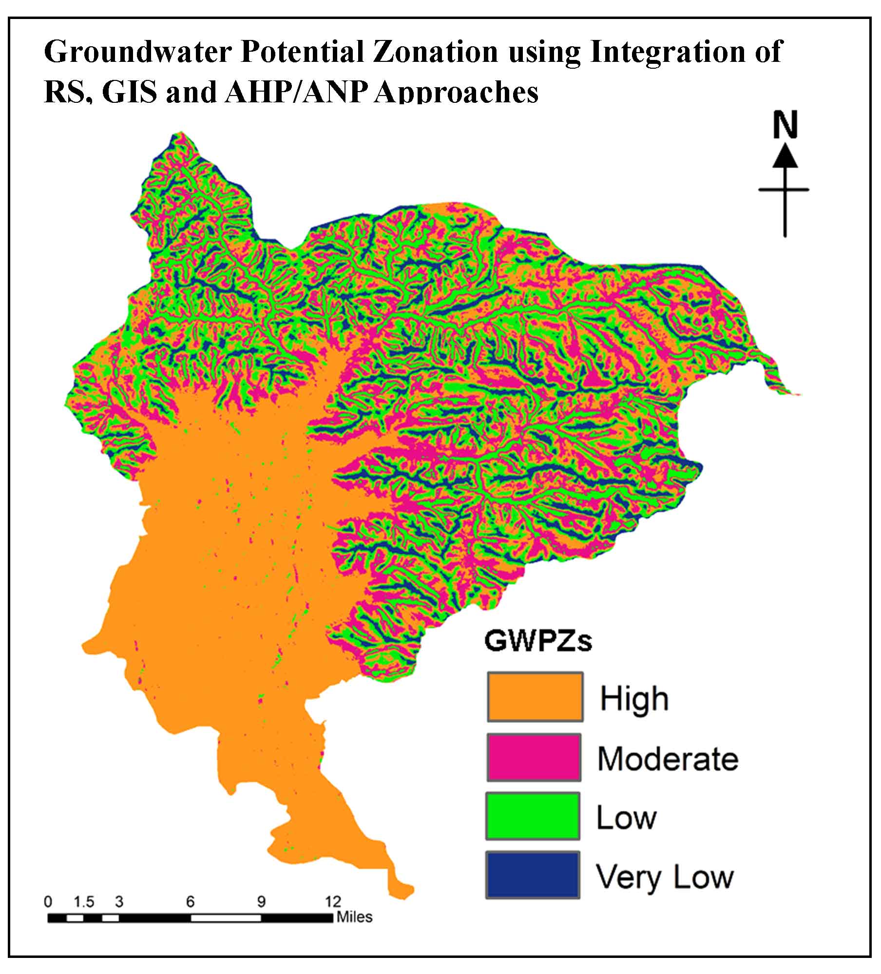
Multi-criteria Decision Making (MCDM) techniques have further refined the associations and interrelationships between different layers of geo-environmental and hydrological inputs working in tandem with the system governing its functioning. Analytical Hierarchical Process (AHP) and Analytical Networking Process (ANP) are the two best and widely used methods of MCDM method. AHP devised by Saaty (1980) as a technique of understanding and deciphering decision-driven problems in socio-economic ‘spaces’ and subsequently solving the issues confronting the societal and institutional structures. AHP is operated when variables are independent, and is best employed in addressing the problems encompassing dependent structure (Yang et al. 2008) whereas ANP likewise formulated through Saaty (1996) deals with modeling judgment based on inputs and measuring them for the derivation of priorities in ratio scale driven in the distribution of association and relationship between the layers used. MCDM with the aid of AHP is the all-pervasive and widely applied technique for assessing groundwater potentiality of any region. Recently, many researchers have applied RS, GIS, and AHP for identifying groundwater prospecting based on multi-parameters (Ghosh et al., 2020; Halder et al., 2020). In the western Himalaya there is overarching trend of depleting stream flow patterns the need for groundwater potential modeling become more relevant for sustainable and realistic review of groundwater resources in the region (Rashid et al., 2020). Groundwater prospecting in the region entails zonation and mapping of different lithological, hydrological and geomorphologic units. Therefore, this work used integration of GIS and RS techniques and AHP/ANP model with respect to hydrogeological, lithological and physiographic geo-database to evaluate groundwater resources of Western Himalaya. The major purpose of this study is to curate a prospective mapping of groundwater resources and assessment by delineating integration of geospatial technology and decision making approach for the whole Kashmir region, making this work the trailblazing one.

2 . STUDY AREA

The study area spread over a swath of geographical area of 1095 km² lies within 34°18′ to 31°40′ N latitude and between 74°30′ and 75°28′ E longitude, which is fringed by the Northern part of Kashmir Himalaya towards the northeastern side, and while as in the southern extremes it spreads throughout the valley (Figure 1). The topography of the area is rugged and steep on the north-eastern side while having the markers of plain landscape on the south-west extremities of area under study. The region is grouped into several physiographic clusters marked by changing elevation bands, slope gradient, foliage, etc. The high altitude mountains, the karewas (lacustrine deposits), foot hills, and low lying alluvial plains comprise the main physiographic formations of the region. The overall altitude of the region varies from 1550 m to ~1774 m (MSL). The variability in the climatic and geomorphological diversity of the region acts as the repository of hydrogeological resource distribution. The climatic regimes have been considered as the average of all the three neighboring weather stations of Gulmarg, Kupwara and Srinagar. The mean maximum temperature in summer is generally 25.82°C, and minimum averages 4.60°C in winter. The month of January being the coldest month displaying lowest mean minimum temperature (4.53°C) and mean maximum temperature (4.60°C), respectively. The rainfall patterns (mean monthly) is being recorded high in the month of March (170 mm) and low in the month of October (42.90 mm). The current water supply needs are mostly catered by groundwater sources with the existing mountainous springs being found all over the area. Central Groundwater Board, the organization designated for quantifying and state of groundwater in country does not have a clearly defined assessment carried out in the region. This study further gets much impetus in attempting to have the summative prospecting off groundwater resources in the region.

Figure 1. Study area

3 . METHODOLOGY

The groundwater flow regimes valley based physiographic configurations with relatively steep slope trajectories are mostly determined by the land use patterns, topographic position, slope settings, and the suitable conditions for groundwater storing capacity. Therefore, is imperative that the appropriate influences are selected to classify the regions favorable for groundwater availability. The final output map was generated by integrating the database generated from satellite and subsequent on-ground datasets.

3.1 Datasets

• Shuttle Radar Tropical Mission Digital Elevation Model (SRTM DEM) having resolution (spatial) of 30 m was employed to generate the thematic layers of slope, drainage and lineament.
• Geocoded Landsat 8 (OLI) dataset with 15 m resolution (acquired May, 2018) on 1:25,000 scales and visual interpretation being carried on the basis of shape, texture, tone and drainage pattern.
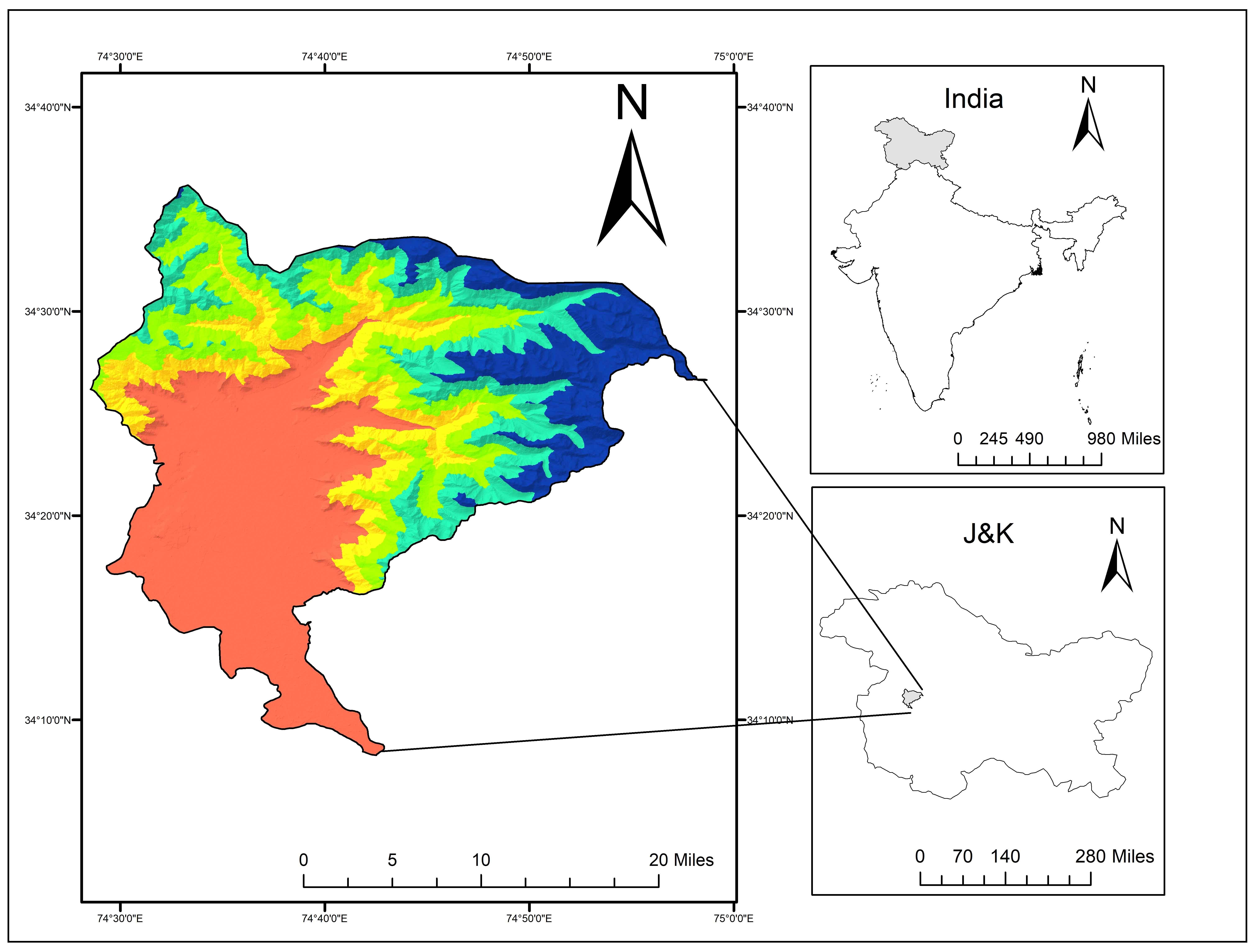
• Survey of India (SOI) map (topographic) sheet of the Bandipora District, Kashmir Valley on a 1:50,000 scale with topo-sheet numbers in the swath of 43 J/7 to 43 J/15 and for referencing Google Earth pro was used to identify the features more accurately.

3.2 Thematic Layers

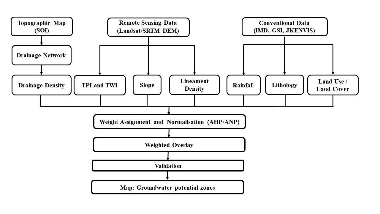
Different hydrogeological factors determine the occurrence and regenerative capacity of groundwater storage (Mohammadi-Behzad et al., 2018). Groundwater potential assessment zonation in the region is done with aid of existing data of eight thematic layers. Hence, the various hydrogeological controlling factors such as lithology, slope, drainage density, lineament density, land use land cover (LULC), Topographic Position Index, Topographic Wetness Index and rainfall are chosen for evaluating groundwater prospects of the area. After selection of layers, diverse datasets (satellite imagery, field data, etc.) are generated from various national and state government institutions including other respective spatial data centers. Subsequently, these hydro-geological layers of eight factors are created and then reclassification analysis is done in ArcGIS 10.3 and additionally the AHP/ANP technique is used for allocating weight of each layer and their corresponding sub-classes as influencing factors governing the groundwater potentiality of the region. The methodology used for estimation of groundwater potential segments is presented in figure 2.

Figure 2. Methodology

3.3 Weights Using AHP/ANP Hierarchy Model

ANP is the decision making technique designed for hierarchical framework of parameters subsequently grouping them for having the pair-wise relative importance of factors and curating of the results based on the judgments made (Saaty, 2004).

There are more than five classes in every thematic layer indicating the complex nature of interrelationship between each sub-class categories. Therefore, the ANP method has been employed for discerning the relationship between all the eight thematic layers used in the study and the identification of respective classes using AHP. The following steps were involved in having the comprehensive hierarchy and derivation of weights for every layer and their corresponding classes:

Step 1: Model Construction

On having the purview of existing literature available on the groundwater potential mapping several methods and modes have been devised accordingly. While constructing the model, decomposition of predefined thematic layers comprising of various individual sub classes of every single theme is used for building a linkage grid of the process.

Step 2: Generating the derived pair-wise association matrices

The determination of values having relative importance are done with the help of Saaty’s scale 1-9 (table 1), wherein 1 represents the score in which two themes have equal importance between them and the score of 9 indicating extreme importance of one theme in comparison to the other (Saaty, 1980).

Table 2 illustrates a prioritization process of matrix in the comparative analysis of classes. A matrix based on pairwise comparison of specified layers is then derived with the help of Saaty’s nine-point scale for groundwater availability in the region. The AHP comprehensively incorporates the idea of uncertain elements in judgments by using consistency index and the principal eigenvalue (Saaty, 2004). Saaty also devised a mechanism for measuring consistency, termed Consistency Index (CI) as degree or aberration in consistency by applying the following equation 1.

\(CI = {\lambda max - n \over n-1}\)                          (1)

where, n represents number of classes and λ max reflects largest eigenvalue of the pairwise comparison matrix. Consistency Ratio (CR) aids in the measurement of consistency in pairwise comparison matrix as represented in equation (2).

\(CR = {CI\over RI}\)                                                  (2)

where, RI is the Ratio Index. RI value of different n values is shown in table 3.

The acceptance level of inconsistency is deemed perfect if the CR value is equal to or smaller than 0.1. If the values exceed 10% of results, the judgment has to be revised.

The pairwise comparison of CR given in table 2 is 0 inferring data is perfectly consistent. The weights of detailed hierarchy of weights and the Consistency Ratio are illustrated in table 6.

Step 3: Construction of ANP Super-matrix

After curating of the pairwise comparison matrix, construction of super-matrix for ANP process is done for representation of relative prioritization of layers. The basic super-matrix of column based eigenvectors is finalized from matrices of pairwise comparison layers. Assuming a system of n elements with each of them having an influence or getting influenced by all or some of the components the function which determines the interaction of the whole system. Let the component of a decision matrix system symbolized by S k, k = 1, 2,...,n. For each component, there exist m k elements denoted as e k1, e k2... e kmk. Now, the impact of S k can be represented as given in equation 3.

The interdependent influence for the relative prioritization of various classes was done by entering the priority vectors (local) in the suitable columns. A super-matrix generally is a matrix with partitioned form with each segment of matrix representing a connection concerning the two bunches (Sun et al., 2007; Wang et al., 2009) preceded by normalization process (Table 4). For obtaining the weighted super-matrix (Table 5), each columnar segment of the matrix is first averaged with the product of the analogous weights and then respectively normalization is done. In order to achieve the absolute aim of relative priorities, the limit super-matrix is realized by raising the weighted (super-matrix) to power by the product of itself. The limit super-matrix is finally prepared when the rows have the equal value as presented in table 6.

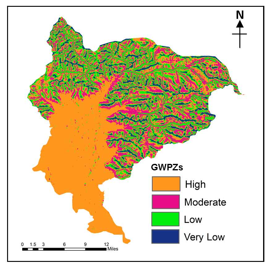
3.4 Weighted Overlay Analysis for Groundwater Potential Zonation

The groundwater potential index (GWPI) is calculated with the application of weighted linear permutation (Machiwal et al., 2011) which is as follows:

\(GWPI = {\sum_{i=1}^{n}\sum_{j=1}^{m}[a_i (\beta_i{_j}X_i{_j})]}\)             (3)

where, \( {\beta_i{_j}}\)  = weight of the j^th class of i^th theme obtained by AHP and \({a_i}\)  = weight of the i^th theme obtained by ANP, n = total number of thematic layers, and m = total number of classes in a thematic layer, \( {X_i{_j}}\)  is the pixel value of the j^th class of the i^th theme.

The validation of groundwater availability zonation is done by preparing the final delineation map with areas being identified for rich and abundant groundwater source regions by the geographical coordinates of the study area (table 8).

3.5 Criterions

3.5.1 Lithology

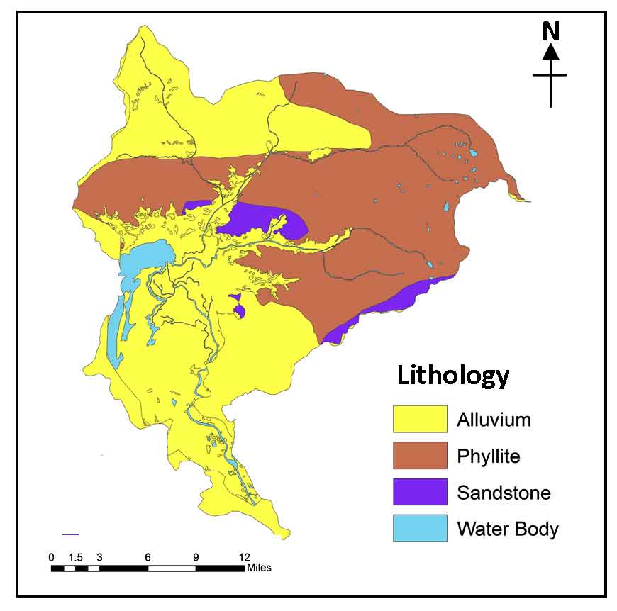
Lithological control reveals several typologies of landforms, geomorphic features and the subsequent hydrogeological settings which aid in the interpretation of the structures, strata as well as lithological composition governing groundwater distribution (Patra et al., 2018). The lithology map is curated from the Geological Survey of India (GSI) district resource map series. The main lithological features found in the district are alluvium, phylite, sandstone (Figure 3). The alluvium is mostly found in the northern and southern part of the district whereas phyllite and sandstone is more prevalent in central and north-eastern part of the district. Alluvium and water body have good to moderate groundwater presence and are given higher ranks in comparison to the other factors (Table 7).

Figure 3. Lithology

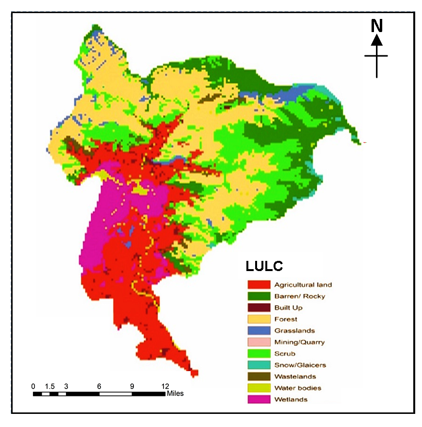
3.5.2 Land Use Land Cover

Land-use land cover (LULC) pattern is one of the significant factors influencing the prospect of groundwater rejuvenation mostly defining the setting of low, medium and high rates of permeation in sub-surface environment. The land use map of the study area is digitized using Landsat 8 (OLI) satellite imagery and based on the inferences ten classes of land use pattern is classified, namely, forest area, mining area, built up area, agricultural area, water body, wasteland, scrub, forest, barren/rocky, grasslands, mining/quarrying and wetland (Figure 4). Water bodies, succeeded by agricultural land use and forest area being the high source zones for groundwater flow are given the highest precedence in ratings, whilst, the low importance classes are built-up area, mining/quarrying area and barren rocky/waste land with respect to the groundwater presence (Table 7).

Figure 4. Land use land cover

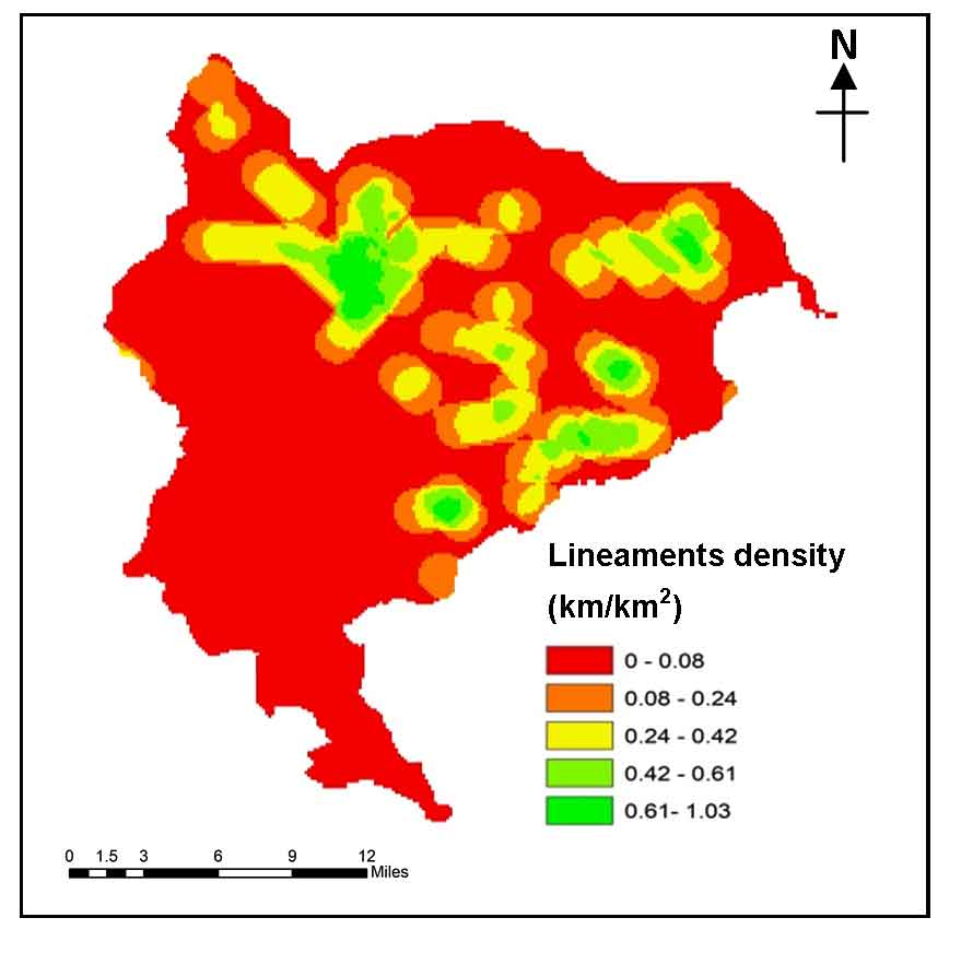
3.5.3 Lineament Density

The spatially enhanced landsat-8 OLI image is imported into the PCI Geomatica 2014 software for lineament extraction. The lineament abstraction procedure (canny edge) of PCI Geomatica software comprises of threshold analysis, edge recognition, and curve removal stages. Structural/tectonic processes give rise to lineaments and the straight faced linear structures having effective secondary penetrability add to the groundwater recharge and flow (Suganthi et al., 2013). The resulting lineament density map is then used for computation of lineament density (L) using the equation 4.

  \(L = { \sum_{i}^{i} (^n_1) L_i / A (km/km^2)}\)                             (4)

where Ʃ \({L_i}\)  denotes the total length of lineaments, A is unit area of lineaments. The lineament density ranges then aid in the generation of the lineament density map of the study area. The lineament density value ranges from 0 to 1.29 km/km² (Figure 5) with higher lineament density values representing higher presence of groundwater and therefore allotted higher rankings (Table 7). The lineament density ranges from 0-0.9 to 0.69 to 1.29 km/ km² and is evenly spread with majority of lineaments covering the north and north-eastern regions of the study area.

Figure 5. Lineament density

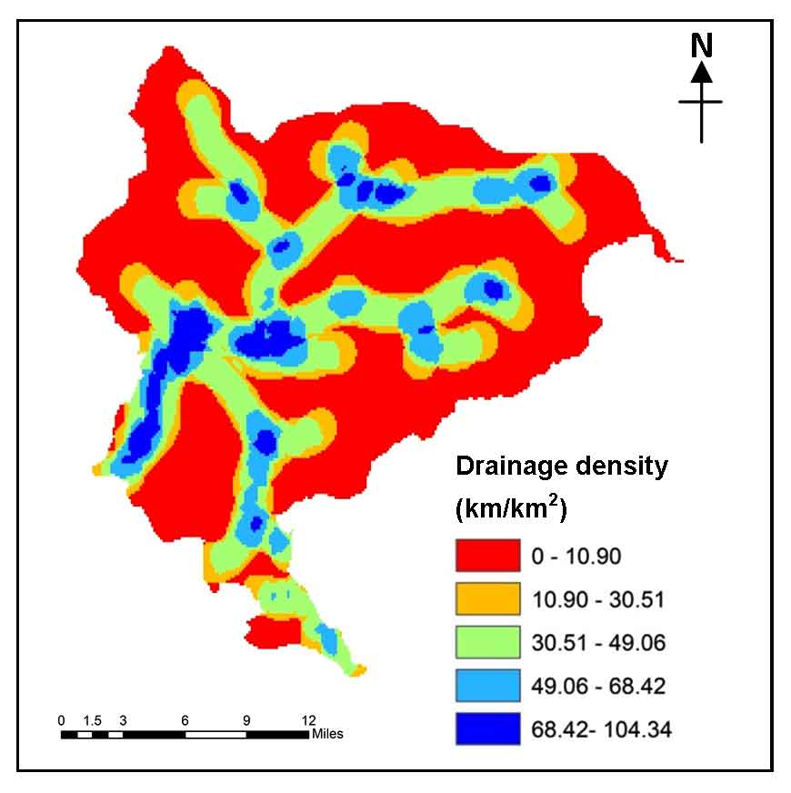
3.5.4 Drainage Density

Drainage density has a direct bearing on land use pattern, topography and geomorphology (Mundalik et al., 2018) and has inverse relation with permeability (Agarwal et al., 2013) thus heavily influences in the process for delineation of GWPZ. Drainage density measure is defined as “the ratio of the sum of lengths of streams to the size of area of the grid under consideration” (Mogaji et al., 2014). Drainage network of the study area is generated from filled and interpolated DEM (30m resolution) by operating the Arc hydro and line density tool in ArcGIS 10.3 and the resultant drainage network is further used to calculate the drainage density (D) as per the equation 5.

\(L = { \sum^{i}_{i} n_1 D_i/ A (km/km^2)}\)                                (5)

where, Σ \(D_i\)  is the sum of lengths of streams in the mesh i (km), and A is the area of the grid (km²).

The drainage density after computation is used to produce drainage density map then and further re-classified into four classes such as 0-1.25 km/km², 1.25-2.5 km/km², 2.5-3.75 km/km², >3.75 km/km², correspondingly (Figure 6). The drainage of the study area mostly follows the radial converging pattern and forms a complex stream network due to the presence of Wular Lake which acts as the centripetal source for most of the water bodies.

Figure 6. Drainage density

Considering the drainage density as influencing factor the study area mostly falls in high drainage density network in the class of 35 to 76 km/km² and is assigned the lower rating and the area having low drainage density is given higher rating due to the fact of providing less surface overflow and high permeation of water within the region (Table 7).

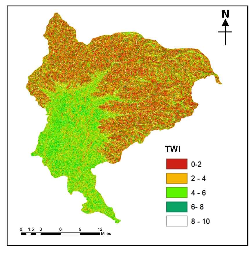
3.5.5 Topographic Wetness Index

Beven and Kirkby (1979) did a pioneering work in the field of hydrogeology by developing TWI within run-off systems. Spatial distribution of wetness conditions can be gauged from this index. More precisely, “it is the ratio between the slope and specific catchment area” (Beven and Kirkby, 1979). The TWI is a secondary index (topographic) that has been extensively computed to explicate the influence of topographic settings on the positioning and size of saturation source in overflow capacity generation that’s why it is also called as secondary topographical attribute. TWI has been broadly applied for groundwater prospective planning and assessment (Davoodi et al., 2013; Nampak et al., 2014) and defining wetness forms geographically (Pourghasemi et al. 2012a, Pourtaghi and Pourghasemi, 2014). This index replicates the behaviour of water to amass at any pour-point and the predisposition of gravitational forces for the movement of that water downstream (Pourghasemi and Pradhan et al. 2012). The terrain profile generally determines the distribution of water in water accumulation areas thus TWI is directly proportional to groundwater incidence. The TWI is defined according to the equation 6 (Moore et al., 1991):

\(TWI = In (As/tan\beta)\)          (6)

where, as is the specific catchment area (m/m) and β is the slope gradient (in degrees) (Nampak et al., 2014). Within the study area, TWI was classified into five classes (Figure 7).

Figure 7. Topographic wetness index

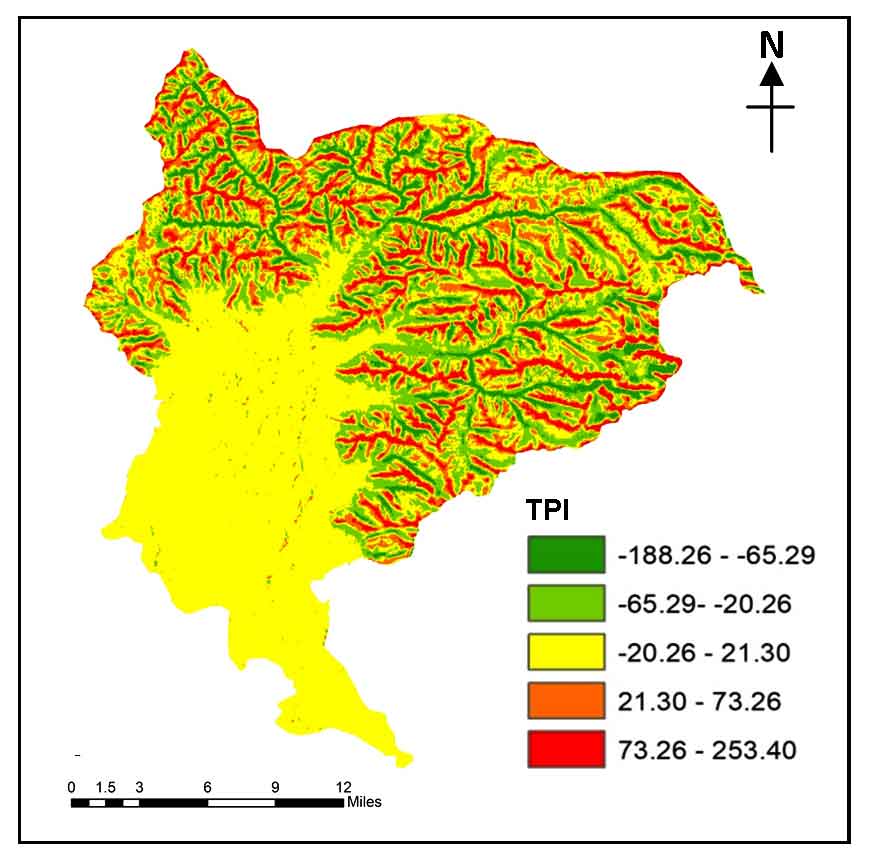
3.5.6 Topographic Position Index

Topographic Position Index (TPI) is the conversion technique in which the rise of each pixel in a DEM to the mean height of an identified proximity around that pixel is linked. TWI is defined as “an inherently scale-dependent phenomenon that gives the positioning of upslope and downslopes attributes of any region” (Guisan et al., 1999). At the top (hilly terrains) higher TPI values in the study area are found, while as in the bottom (valley) low TPI values are found and the TPI values near zero are found on either flat ground or medium slope (Figure 8). The area is divided into five classes ranging from -188.26-45.29 to 73.26-250.40 with flat slopes considered favorable for groundwater potential.

Figure 8. Topographic position index

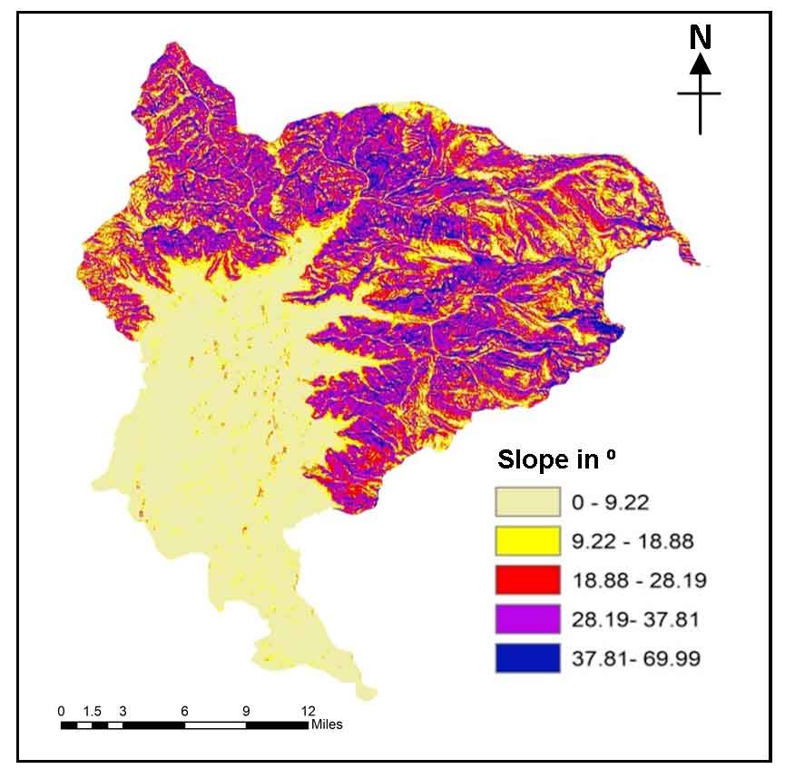
3.5.7 Slope

Slope angle largely controls the groundwater recharge processes according to most of the studies (Ettazarizini and El Mahmouhi, 2004; Prasad et al., 2008), hence, it is a significant factor for the spatial predictability of groundwater potentiality. The slope map of the area was curated based on DEM analysis using the Spatial Analysis tools in ArcGIS 10.3. Deriving from the Jenks natural breaks classification, the slope angle map was grouped into six classes varying between zero and 69.9 degrees. Less value classes are consigned higher rank due to almost flat trajectory while the maximum value classes are characterized as lower rank due to comparatively high run-off (Figure 9).

Figure 9. Slope

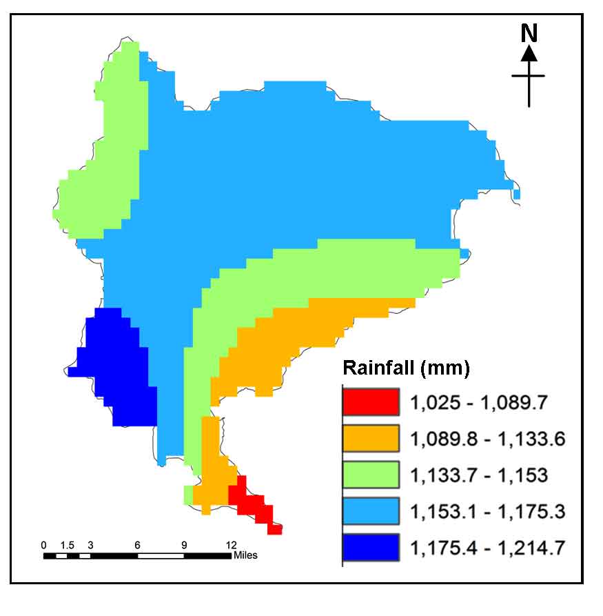
3.5.8 Rainfall

Rainfall map of the region was generated using ordinary Kriging method (Bargaoui and Chebbi, 2009) in geospatial environment based on daily IMD data. The time period (1970-2018) was used for interpolating the perception scenario of the region on annual time scale as shown in (Figure 10) with north-western region receiving substantial amount of rainfall.

Figure 10. Rainfall

4 . RESULTS AND DISCUSSIONS

4.1 Groundwater Potential Zones

The groundwater potential zonation map after the geospatial operations of North Kashmir is generated by integrating eight thematic layers with respect to the relative prioritization abstracted from subjective weights based on the review of literature method. The overlaying of GWPZ was done with help of following equation .The following equation was used to examine the final output map of the area.

 \(GPM=(MC1w×SC1r)+ (MC2w×SC2r)+ (MC3w×SC3r)+ (MC4w×SC4r)\)

\(+ (MC5w×SC5r)+ (MC6w×SC6r)+ (MC7w×SC7r)+ MC8w×SC8r\)    (7)

where, GPM is the groundwater potential map, MC1-MC7 is the main criteria (1-8 thematic layers) w is the weight of thematic layer, SC1-SC8 is the sub criteria of each thematic layer map and r is the sub criteria class rating. The thematic layers are same as defined above (lithology, Topographic Wetness Index (TWI), Topographic Position Index (TPI), slope, drainage density, lineament density, LULC and rainfall)

Accordingly, with the help of Jenks natural breaks method, the map being developed is then further divided into four zones based on their relative potential namely very low, low, moderate and high (Figure 11). The distribution area of potential zones is prepared (Table 9) in ArcGIS 10.3. It is inferred that 12.29%, 31.91%, 16.23% and 39.57% of the aggregate area comes under very low, low, moderate and high GWPZ’s, correspondingly (Table 8). The final output map infers that, the eastern, central and lower southern region of the study area display mostly moderate to high groundwater potential zones. While comparing the GWPZ map in the regions from moderate to high groundwater potential with respect to the prevalence of various hydrogeological conditions indicate that the aquifers of central and southern regions which are covered by water bodies, forest and agricultural land use. Similarly, in these zones, geomorphological controls dominate in the prevalence of features such as half weathered and rugged terrains, low drainage density (0-10.90 km/km²) comparatively more rainfall distribution (1175.4-1214.7 mm/annum), flatter slope (0-9.22°), the existence of loamy and coarse loamy type soil also encourages the high groundwater prospects. Similar findings have been found in the number of studies suggesting the relevance of geomorphological and hydrological characteristics in the identification of groundwater potential zones (Kumar and Krishna, 2018; Das et al., 2018; Nag and Ghosh, 2013). Other studies have also concurred with the land use land cover being significant factor too in the groundwater potentiality (Mukherjee et al., 2012; Yeh et al., 2016).

 

Figure 11. Groundwater potential zones

 

With respect to zones having moderate potential in terms of groundwater, there expanse can be observed in the central and parts of north eastern regions which mainly encompasses agricultural lands overlying flatter to gentle slope (18.88-19.25%), relatively low drainage density (30.51-49.06 km/km²) etc. Similarly from results achieved from the final GWPZ reveal that north and north-eastern regions fall under the category of poor groundwater potential zonation with relatively impermeable formation, forests, higher slope values (37.81-69.09°) and higher elevation with low potential of infiltration which subsequently leads to poor groundwater storage capacity in this region. This inference corroborates with other reported studies while indicating the hilly terrains, elevation, topographic, slope and impermeable formations in as the factors responsible for poor groundwater potentiality (Shekhar and Pandey, 2015; Ibrahim-Bathis and Ahmed, 2016). Around 55% of the area falls in the moderate to high groundwater potential category which covers major portion of central and southern region and few pockets of the north eastern extent.

 

Table 8. Area under different GWPZs

Classes	Area
	km2	%
High	420.40	39.57
Moderate	180.24	16.23
Low	351.31	31.91
Very Low	142.11	12.29

 

 

4.2 Validation

For validating the accuracy of potential zonation map of study area, geo-coordinates of groundwater sources are validated on the final output groundwater potential map (Figure 12) on the basis of existing and the final output map status. Receiver Operating Characteristic (ROC) curve investigation was applied for quantitative validation by comparative assessment of the existing groundwater samples with the results from groundwater potential map developed by MCDA (Pourtaghi and Pourghasemi, 2014). For corroborating the expected groundwater prospect map 31 existing sampling were taken and used for ROC curve preparation. Figure 13 shows the ROC curve of the GPM obtained using AHP/ANP method. In ROC curve, the true positive rate (sensitivity) is plotted in function of the false positive rate for different grading of a parameter. The sensitivity pair concerning the particularity of decision matrix, points are drawn which represent the same. The area under the ROC curve (AUC) is a basically the measurement of how parameters differentiate between two diagnostic clusters factored in for validation. The connexion amid AUC and prediction accurateness can be precised as (Naghibi et al., 2015): Poor (0.5-0.6); average (0.6-0.7); good (0.7-0.8); very good (0.8-0.9); and excellent (0.9-1). The final validation of findings exhibited that AHP/ANP technique has a relatively significant accuracy (prediction) of 0.755. The spatial positioning of categories with its corresponding potential status to respective zones is given which gives the overall scenario of the groundwater resources in the area. Respectively, from this data different categories of groundwater potential zones can be identified on the basis of very low, low, moderate and high groundwater potential. Hence, groundwater potential validation results corroborate significant consistency of the accurate final output map generated from the robust GIS based weighted overlay approach integrated with AHP/ANP model of MCDM method.

 

Figure 12. Sampling sites

 

Table 9. Accuracy Assessments

Location		Groundwater Potentials		Agreements
Longitude	Latitude	Ground observations	Estimated
74.55256	34.50261	Very Low	Very Low	True
74.55149	34.48437	Moderate	Very Low	False
74.56222	34.48593	Very Low	Very Low	True
74.58342	34.52026	Low	Very Low	False
74.59444	34.50059	Very Low	Very Low	True
74.59111	34.50278	Very Low	Very Low	True
74.65681	34.44004	Low	Very Low	False
74.65919	34.46363	Very Low	Very Low	True
74.63979	34.43046	Low	Low	True
74.69777	34.41439	Low	Low	True
74.66888	34.36805	Low	Low	True
74.67804	34.32949	Very Low	Low	False
74.69099	34.32932	Low	Low	True
74.67199	34.28399	Moderate	Low	False
74.64345	34.21784	Low	Low	True
74.59514	34.51568	Low	Moderate	False
74.71476	34.45540	Moderate	Moderate	True
74.65292	34.46280	High	Moderate	False
74.69320	34.41335	Low	Moderate	False
74.66091	34.37405	Moderate	Moderate	True
74.61447	34.46214	Moderate	Moderate	True
74.59037	34.22418	High	High	True
74.58144	34.24477	Very High	High	False
74.62359	34.27068	High	High	True
74.62144	34.23192	High	High	True
74.63287	34.20113	Very High	High	False
74.63467	34.18126	High	Very High	False
34.20088	34.20088	Very High	Very High	True
34.20784	34.20784	Very High	Very High	True
34.48476	34.48476	Very High	Very High	True

 

 

Figure 13. Receiver operating characteristic curve

 

 

5 . CONCLUSION

The application of multi-criteria decision making prospects i.e. AHP/ANP model integrated with remote sensing based approach in Western Himalaya, India opens up the new horizons for hydrogeological and geo-environmental significance in the region. The study area has the identity of being the resource rich zone with the prevalence of horticultural, agriculture and commercial sectors thriving in substantial rates. The augmentation in the water needs have drastically shifted the focus to groundwater harvesting and management. For evaluation of the groundwater resources prospecting in the region and scientific application in the impending water security issues, delineation of groundwater potential zones in the region becomes imperative. Firstly, GWPZ map is prepared which shows 420.40 km² (39.57%), 180.24 km² (16.23%), 351.31 km² (31.91%) and 142.11 km² (12.29%) of total area fall under high, moderate, low and very low potential zones, respectively. The low potential areas are mostly abstracted more and have the anthropogenic pressures impending more. This demands a sustainable and viable withdrawal practices required for having the judicial and appropriate consumption of groundwater resources in the region. Around 560 km² (55%) of the study area (south central and eastern part), represents moderate to high groundwater potential zone attributed to groundwater conditioning patterns of land use including forest, agricultural area and converging radial pattern of drainage network. In contrast to that, the impermeable condition typologies and presence of geomorphological features (barren mountains, hard-rock patches, karewas) which is marked on the Northeastern side of the area with some disseminated patches in the extreme north trigger to poor groundwater presence of the area . Thereafter, map validation is done for having the accurate perusal of the different potential zones bases on the integration and respective weight of different hydrogeological factors for carrying out the comprehensive assessment of groundwater resources of the region. Finally, validation of the geo-database is achieved by tallying the inferences from the final output map with available geo-coordinates of groundwater source regions. Various agencies and several institutions at different levels both at national and international have utilized the application of remote sensing and GIS for the timely and precise evaluation of the management and water resources planning such as delineation potential of groundwater zones, risk evaluation of flood events, analysis of drought patterns across the world. Furthermore, there is scant attention being invested into the water resource planning and management in the area particularly in the groundwater resource explorations exacerbated by complex topographic configurations, it becomes thus highly imperative to have the scientific and modern geospatial database generation for the efficient and timely appraisal of groundwater scenario in the region. With the application of geospatial technology hyphenated with the decision making techniques these resources can be harnessed and utilized prudently as burgeoning population and altering hydro-meteorological conditions have accentuated the demands for water consumption. The need of the hour is to have the summative and robust prospecting for groundwater resources with the interface both the geospatial and decision making system approach in the region. Artificial recharge techniques and participatory approach can be implemented in these regions with the moderate and low potentiality to increase the groundwater table and thereby preventing it from overexploitation.

Tables

Figures

Conflict of Interest

Acknowledgements

Abbreviations

References