Keywords

Sinuosity , GIS , Channel planform , Bifurcation Ratio

1 . INTRODUCTION

Morphometric analysis deals with a quantitative description of the basin geometry to know initial slope or differences in the rock resistance, structural controls, recent diastrophism, geological and geomorphic history of drainage basin (Strahler, 1964). Morphometry is the measurement and mathematical analysis of the arrangement of the earth’s surface, shape, dimension of its landforms (Clarke, 1966). Nag and Chakraborty (2003) used morphometric analysis to study the influence of rock types and structures in the formation of drainage network in hard rock area. Morphometric analysis has been used to evaluate the groundwater potentiality of the basins in many studies. Geo-informatics using satellite images are used as a suitable tool for morphometric analysis. Many studies have been carried out in morphometric analysis using these new techniques.

A perfect straight river is unusual. All natural rivers have a fundamental tendency to deviate from a straight line and increase their sinuosity. Friedkin (1945) defined the degree of sinuosity of meandering rivers as the ratio of Thalweg length to the air-line. According to Morisawa and Clayton (1985) a plan-form between straight and meandering can be called sinuous. Sinuosity indexes are usually calculated by dividing the length of a reach measured along a channel by the length of a reach measured along a valley (Muller, 1968). Considering the facts above, the study was undertaken to determine and understand the significant morphologic and hydrologic characteristics of Tlawng river basin.

2 . MATERIALS AND METHODS

The Tlawng river basin was extracted from ASTER Globe Digital Elevation Model (GDEM) at 30 m resolution downloaded from ISRO Bhuvan website. Hydrological information was digitized and geo-referenced using Arc GIS tools. Channel sinuosity index is measured by using formula proposed by Mueller (1968). Relief and drainage properties such as stream ordering, stream number, stream length, mean stream length, stream length ratio, Rho coefficient, bi-furcation ratio, drainage density, stream frequency, drainage texture, relief ratio, relative relief, ruggedness number etc. is studied to understand the terrain characteristics.

3 . STUDY AREA

The Tlawng river is the lengthiest river in Mizoram which measures about 185 km within the state. It originates from Zopui hill at 22°51ʹ N latitudes and 92°48’ E longitudes, 8 km east of Lunglei town at an elevation of about 1598 m from MSL (Figure 1). The lowest elevation is about 6 m in Katakhal, where it joins the Barak river. The basin is about 5846 km². It passes through five districts namely Lunglei, Aizawl, Serchhip, Mamit and Kolasib in the state of Mizoram. During the course of its run, several tributaries join laterally. It flows in northern direction. After flowing for about 50 km in Lunglei district it enters Aizawl district near Khawlek village. Tut and Teirei are the main tributaries to the river Tlawng. The Teirei river flows parallel to the Tlawng river for about 40 km before joining the main Tlawng river. After the confluence with tributaries Tut and Teirei from western bank, it joins Barak river in Cachar district of Assam where it is known by the name Dhaleswari river and Katakhal river. It is the main source of water supply for Aizawl city.

Figure 1. Location Map: River Tlawng basin in Mizoram (India)

The Tlawng river basin is characterized by undulating hill ranges with steep slopes in the upper course and moderate to gentle slope in the lower course. The Tlawng river basin is having a tropical humid climate with heavy monsoon rainfall. The average annual rainfall in the study area is about 2450 mm. Soils are generally of sedimentary formation which is sandy, immature and high in acidity. The average annual temperature is around 21ºC.

4 . RESULTS AND DISCUSSION

For the study, streams are ranked as per their order. The morphometric and sinuosity analysis provides information of the geometrical relationship among the stream segments with terrain characteristics and lithological variations.

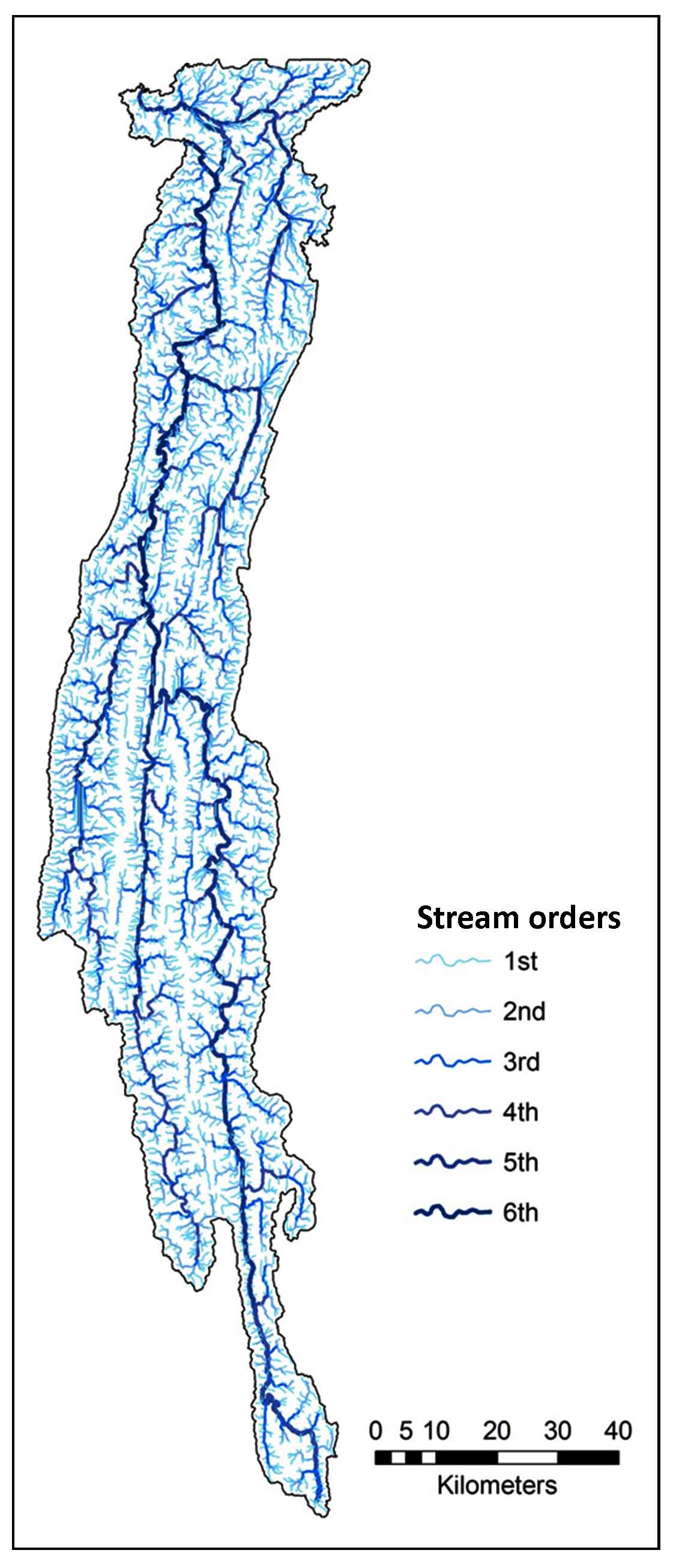
4.1 Stream Orders

Stream order is a measure of the relative size and pattern of channels of a drainage network. This provides an important influence on the relative discharge of streams at any point of a drainage network. In any drainage network analysis, the streams are categorized into different orders in accordance with the number of bifurcations. Various methods of stream ordering were suggested by earlier workers. Davis (1913) proposed a genetic approach to drainage pattern. However, the most important quantitative approach to drainage analysis was proposed by Horton (1945) and Strahler (1952). According to Strahler (1952) perennial streams having no tributaries are termed first-order. When two equal order streams come together, the downstream reach is increased by an order. The main stream through which all the discharge of the water is carried out is the highest order stream. The study area is a 6^th order drainage basin (Figure 2). A total of 7638 streams are identified in Tlawng river basin out of which only  3847 are 1^st order streams. There are 1848 2^nd order streams, 874 3^rd order streams, 443 4^th order, 474 streams, 148 5^th order streams and 148 streams in the 6^th order (Table 1). According to Zaidi (2011), the topography is still undergoing erosion if the number of stream is more, whereas less number of streams indicates   matured topography.

Figure 2. Stream orders

4.2 Stream Number

Stream number (Nu) is the number of stream segments which exist in every order. According to Horton (1945), the number of stream segments of every order forms an inverse geometric relationship with order number. A total of 6736 streams are present in the drainage basin (Table 1). From table 1, it is clear that the number of streams decreases with an increased stream order. The presence of more number of streams in the basin is expected to change the morphology of the channels at many sections influenced by the local topography and high discharge as observed.

4.3 Stream Length

Stream length (Lu) is calculated from the mouth to the drainage divide. The total length of all streams in the basin is 2156.45 km. The 1^st order streams have a length of 3484 km and the stream length of the 2^nd order is 1678 km. The length of 3^rd order streams is 737 km and 4^th order streams have a stream length of 359 km. Fifth order and sixth order streams have a length of 352 and 126 km, respectively. The length of the main channel is about 320 km. The total stream length of first order streams is by far greater than the second, third, fourth fifth and sixth order streams. As proclaimed by Horton (1945) the total stream length of respective orders decreases with increasing order of streams. As more number of streams is present in higher orders it influences the channel morphology of the lower orders in the downstream sections.

4.4 Mean Stream Length

A dimensional property showing the characteristic size of components of a drainage network and its contributing watershed surfaces is known as mean stream length (Lsm) (Strahler, 1964).  From table 1, it is observed that the mean stream length ranges from 0.85-1.97. Normally, Lsm increases with increasing stream order, but the deviation observed may be due to slope and topographic variation in the different segments of the stream.

4.5 Stream Length Ratio

The mean length of the one order to the next lower order of the stream segments is called stream length ratio (Rl) (Das et al., 2011). A difference in the stream length ratio from one order to another order means the development of the late youth stage of streams. The stream length ratio in the study area varies from 0.42-1.79.

4.6 Bifurcation Ratio

The ratio of the number of streams in a given order to the number in the next higher order is known as bifurcation ratio (Rb) (Horton, 1945). It is considered as the index of relief and dissection Horton (1945). Lower bifurcation ratio means that  the drainage basin have flat or rolling plain while high bifurcation ratio specifies strong structural control on the drainage pattern and have well-dissected drainage basins (Horton 1945; Fryirs and Brierley, 2013). The bifurcation ratio of Tlawng drainage basin ranges from 0.93 to 3.20. The mean bifurcation ratio of the basin is 2.05. The higher the bifurcation ratio, the shorter is the time taken for discharge to reach the outlet. Hence peak discharge will be high. This will lead to greater probability of flooding. Hence, Tlawng river has a low chance of flooding as it has a low bifurcation ratio.

4.7 Rho Coefficient

The Rho coefficient is an important factor connecting drainage density to physiographic development of a drainage basin. It enables the calculation of storage capacity of drainage network (Horton, 1945). The Rho value of the Tlawng river basin is 0.50 which indicates low to moderate hydrologic storage during floods (Table 1). This might have some effect on the morphological changes of the lower order channels like from 3^rd order streams up to the main channel.

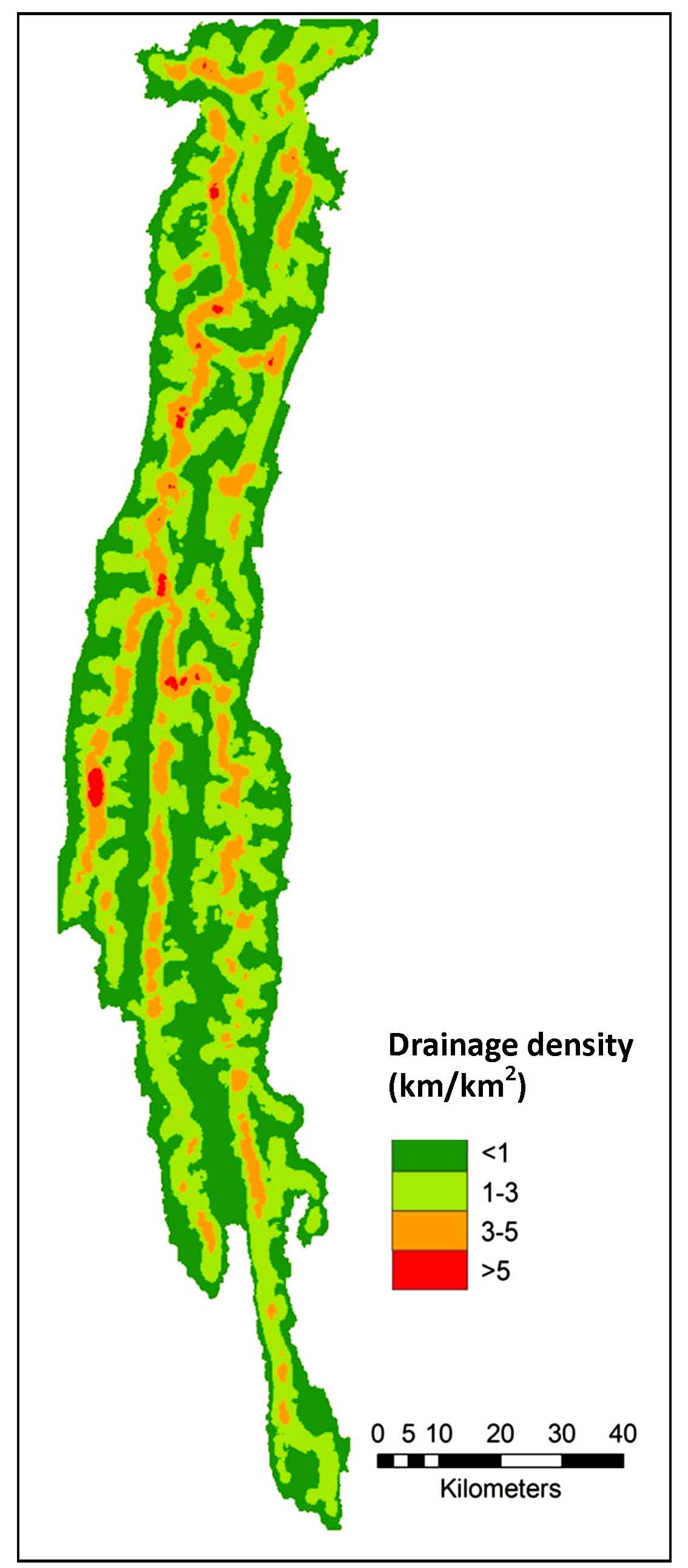
4.8 Drainage Density

According to (Horton, 1945), drainage density is the stream length per unit area in a region of watershed. Drainage density is an important linear aspect of the drainage basin. High drainage density reveals the highly dissected drainage basin and rapid hydrological response to the rainfall events while low drainage density reflect slow hydrological response (Selvan, 2011; Hajam et al., 2013). The study area is divided into four classes of drainage density such as high drainage density (> 5 km/km²) with areal extent of 27 km², moderate drainage density (3-5 km/km²) with areal extent of 735 km^2, low drainage density (1.5-3 km/km²) of 2474 km² and very low drainage density (<1 km/km²) occupies an area of about 2622 km² (Figure 3). The major part of the Tlawng drainage basin has a low drainage density of 1.15 km/ km² covering an area of about 2474 km² which indicate that basin area has a resistant permeable subsurface material and a moderate to thick vegetation cover. Also it is noticed that many tributary streams dried up during lean season.  According to Dingman (2009), low value of drainage density is one of the characteristics of the humid region. Due to major extent of the low and very low drainage density, river Tlawng can be considered as a uniform and steady channel where velocity is almost constant and stream pattern does not change much with time.

Figure 3. Drainage density

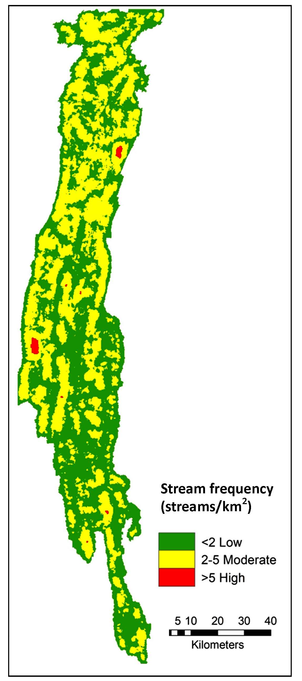
4.9 Stream Frequency

The total number of stream segments of all orders per unit area is known as stream frequency (Sf) (Horton, 1932). The stream frequency value of the Tlawng river basin is 1.30 streams / km² which shows a positive relation with drainage density. Stream frequency normally depends on the lithology of the drainage basin. The study area is divided into three frequency classes (Figure 4), such as high stream frequency (> 5 streams/km²) with areal extent of 24 km², moderate stream frequency (2-5 streams/km²) with areal extent of km², low stream frequency (< 2 streams/km²) of 3259 km². Reddy et al. (2004) stated that low stream frequency values indicate the existence of a permeable subsurface material and low relief. As the area is composed of permeable rocks like sandstones with an average relief of 377 m the Tlawng river basin shows low stream frequency.

Figure 4. Stream frequency

4.10 Drainage Texture

Drainage texture (Dt) is the total number of stream segments of all orders per perimeter of that area (Das et al., 2011). Drainage texture of a drainage basin relies on parameters such as climate, rainfall, vegetation, soil and rock types, infiltration rate, relief and the stage of development (Horton, 1945; Smith, 1950). Smith (1950) has categorized drainage texture into five textures i.e., very coarse (<2), coarse (2 to 4), moderate (4 to 6), fine (6 to 8) and very fine (>8). Areas having low drainage density have coarse texture while areas with high drainage density have fine drainage texture. The drainage texture of Tlawng river basin is 0.88 (Table 3), which falls under vey coarse drainage texture. According to Horton (1945), the more drainage texture more will be dissection and results in increased erosion which can affect the channel morphology at places.

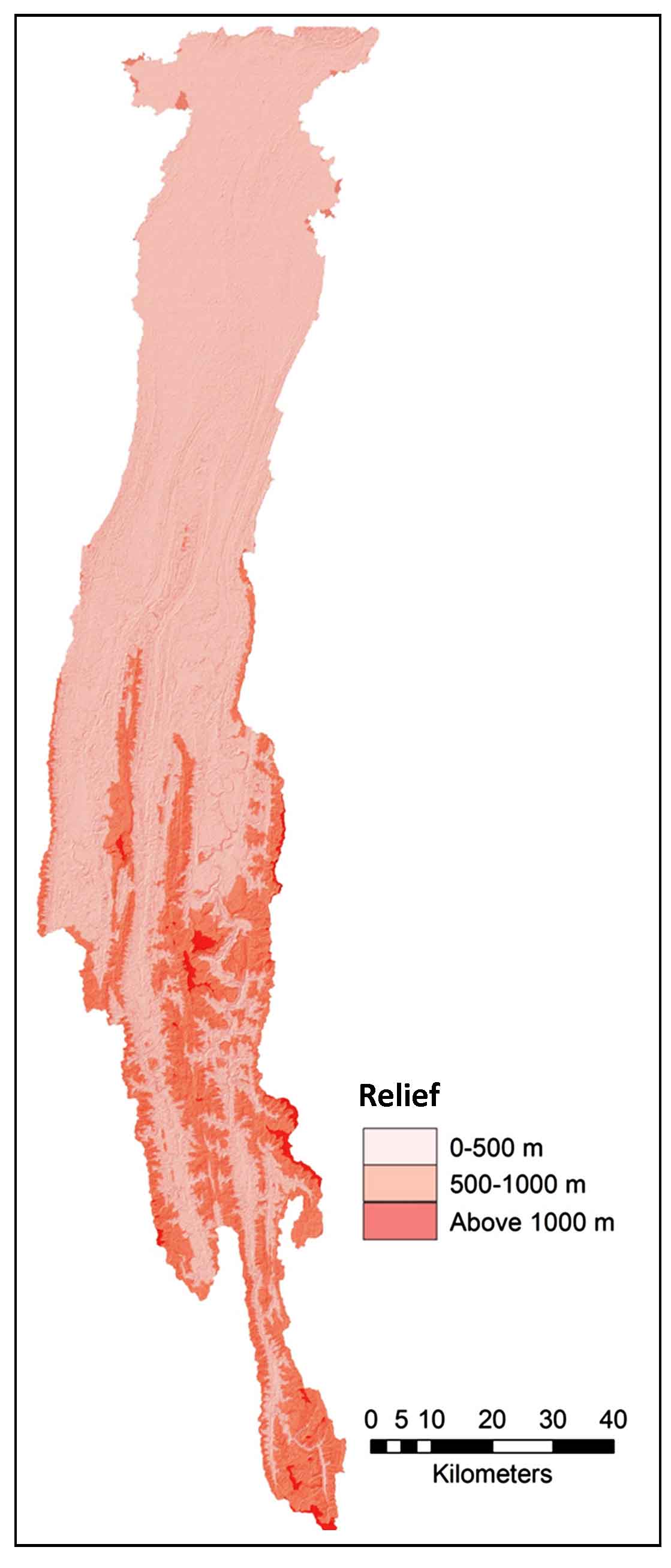
4.11 Basin Relief

Relief is the difference in elevation of any part of the earth’s surface or relative vertical inequality of land surface. Relief is considered as the range in altitude (Smith, 1935). The difference in elevation between the highest point of a basin (H) and the lowest point on the valley floor (h) is called basin relief (Strahler, 1957). The lowest point is 6 m, and highest point is 1598 m and moderate slope and moderate runoff. The relief values have been grouped into three categories such as 6-500 m (low), 500-1000 m (moderate) and above 1000 m (high) (Figure 5).  The relief value 6- 500m zone occupies  about 4456 km²of the basin area, moderate relief region of 500 to 1000 m covers maximum area of about 1239 km²and above 1000 m high relief zone occupies about 60.3 km²of the total basin area. Major portion of the basin area falls under low relief followed by moderate relief and high relief zone covers the smallest area in the basin.

Figure 5. Relief

4.12 Relief Ratio

The relief ratio (R_r) is the ratio between the total relief of a basin and the longest dimension of the basin parallel to the main drainage line (Schumm, 1956). If the relief ratio is high it means hilly region and low ratio pertains to pediplain and valley region (Kumar et al., 2011). Relief ratio of Tlawng river basin is 4.75 (Table 4) indicating moderate relief and moderate slope which might affect channel morphology to some extent particularly, in the lower sections.

4.13 Relative Relief

Relative relief (Rhp), according to Melton (1957) is the ratio between the relief and perimeter of the watershed. Relative relief has been calculated by Melton’s (1957) which is 0.19. This signifies that the land surface has low to moderate slopes. In accordance with the direct relationship between relative relief and denudation rates, it is found that major denudational landforms are found in the northern part (lower course) of the basin. Denudation landforms in the northern part might affect the channel morphology from 3^rd order streams.

4.14 Ruggedness Number

Ruggedness number (Rn) is the outcome of the basin relief and the drainage density and significantly associate slope steepness with its length (Strahler, 1957). Exceedingly high values of ruggedness number are found when slopes of the basin are not only steeper but long, as well (Chow, 1964). The ruggedness number (Rn) of Tlawng river basin is 1.83. Ruggedness number is found to be directly proportionate to relative peak discharge (Patton, 1988).

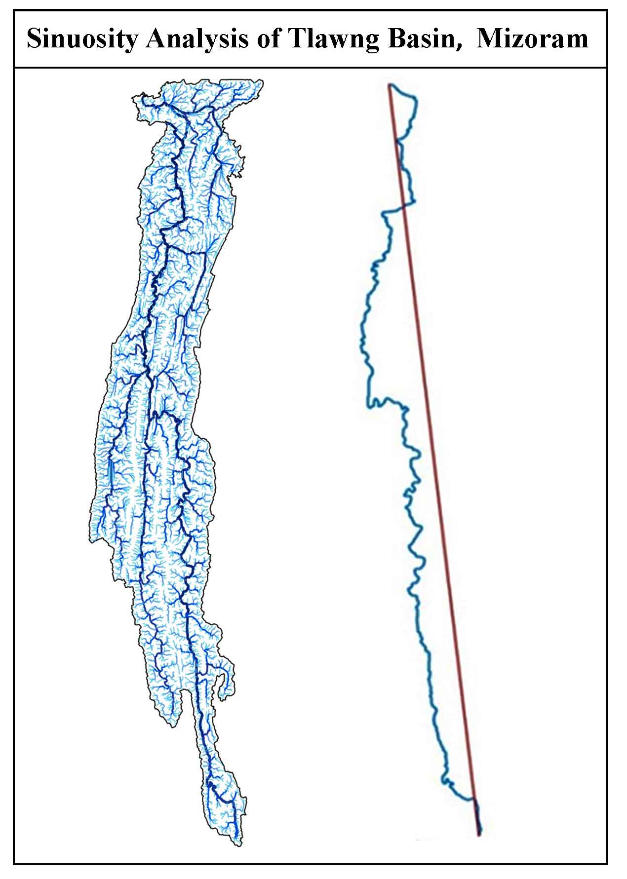
4.15 Sinuosity

Sinuosity is the relation between channel length and valley length. Rivers meander in order to sustain a channel slope in equilibrium with discharge and sediment load. On a meandering river, sinuosity is the ratio of channel length to valley length. According to Keller and Pinter (2002) any tectonic deformation changing the slope of a river valley results in a conforming change in sinuosity to maintain the equilibrium channel slope.

Acording to Muller (1968), channel sinuosity (S) is the ratio between the stream length (Sl) to the valley length (Vl), which is expressed as S = Sl/ Vl. Sinuosity index can be computed as the ratio of the length of channel to length of valley axis (Brice, 1964). According to the Brice (1964), if the sinuosity index of a reach is 1.3 or more, the reach is considered as meandering, a straight reach is having sinuosity index of 1 and reaches which have sinuosity indices between 1.05 and 1.3 are regarded as sinuous.

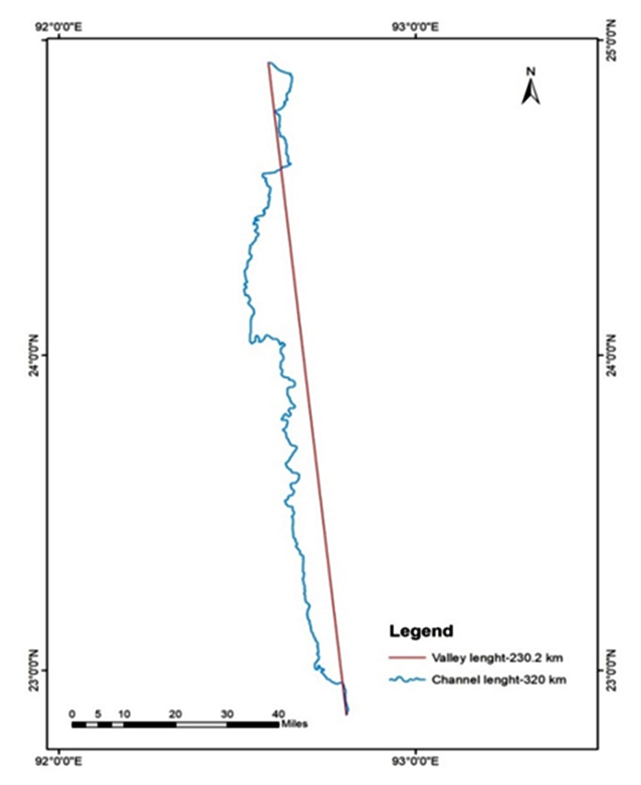
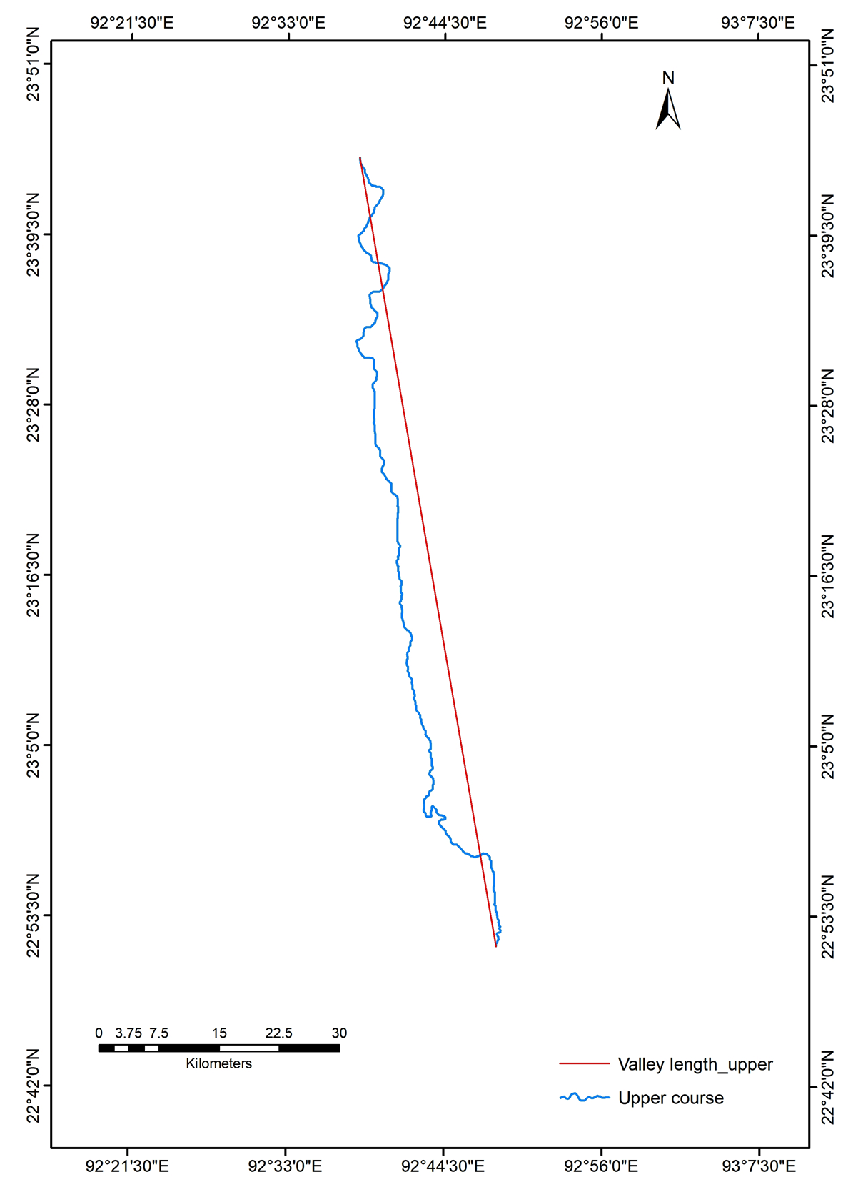
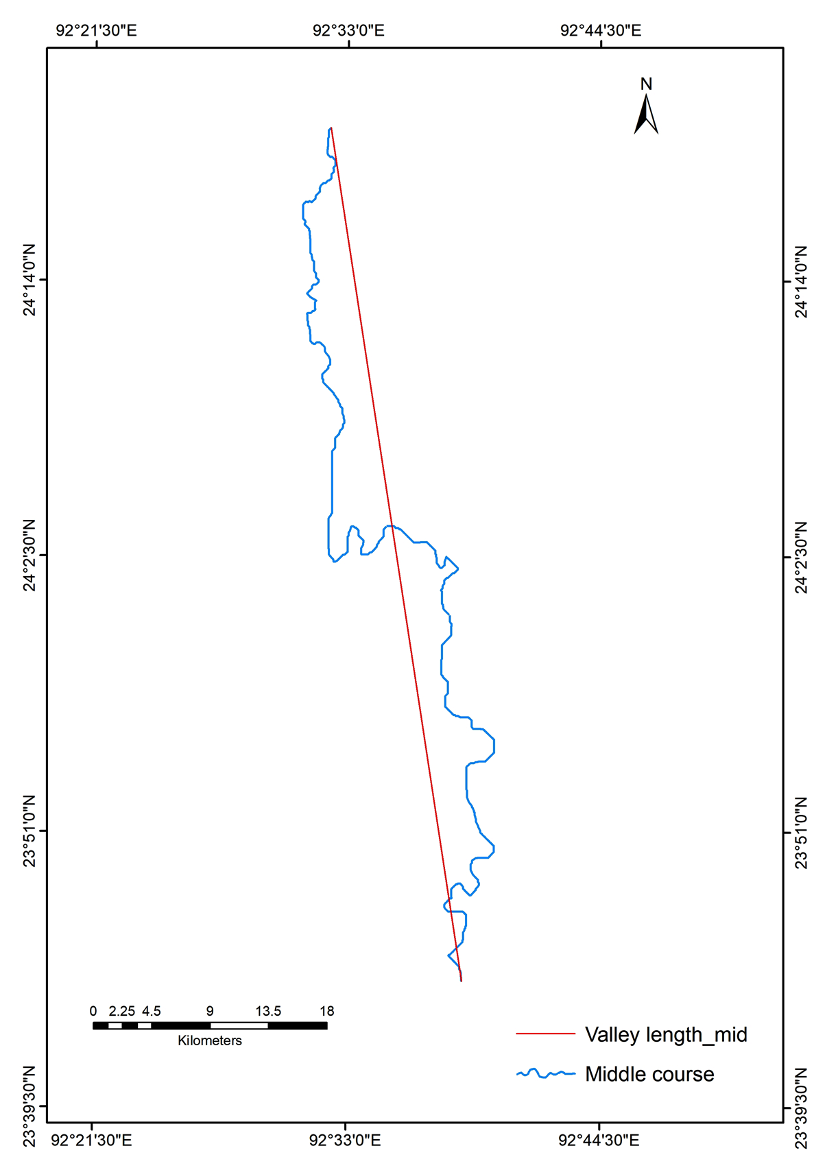
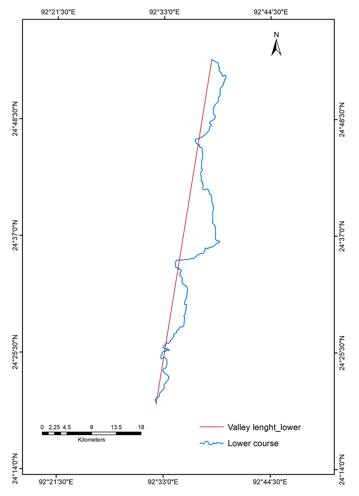
The channel length (CL) of Tlawng river is 320 kilometers from source to mouth while the valley length or air length (VL) is calculated as 230.2 kilometers. Sinuosity index has been computed as the ratio of the length of channel to length of valley axis - CL/VL. The river is having a sinuosity index value of 1.39 (Figure 6; Table 5) which is a sinuous channel (Morisawa and Clayton, 1985). The upper course of the river has a channel length (CL) of 102.77 kilometers and a valley length (VL) 99.8 kilometers. It can be considered as a sinuous channel with 1.03 sinuosity index value. With a sinuosity index value of 1.9 (Table 6) and a channel length (CL) and value length (VL) of 125.742 and 66.51 kilometers the middle course can be said as a meandering channel. The channel length (CL) and valley length (VL) of the lower course is 89.689 kilometers and 67.96 kms, respectively. Its sinuosity index value is 1.31 (Figure 7, 8 and 9).

Figure 6. Sinuosity index of Tlawng river

Figure 7. Sinuosity: Upper course

Figure 8. Sinuosity: Middle course

Figure 9. Sinuosity: Lower course

5 . CONCLUSION

The sinuosity and morphometric parameters estimated using GIS helped us to comprehend several terrain characteristics like nature of the bedrock, infiltration capacity, runoff, etc. The area is having a permeable sub surface. Due to low bifurcation ratio the river has low potentials of flooding. A total 6736 streams are identified in Tlawng river basin which indicates that the topography is still undergoing erosion (Zaidi, 2011). The stream frequency is low which is showing a positive relation with drainage density. Due to major extent of the low and very low drainage density Tlawng river can be considered as a uniform and steady channel where velocity is almost constant and stream pattern does not change much with time. The study will be useful for flood management, ground water assessment, soil erosion assessment and water resource management.

Tables

Figures

Conflict of Interest

Acknowledgements

Abbreviations

References