Keywords

Agriculture , AHP , GIS , Land Suitability , Remote Sensing

1 . INTRODUCTION

Precision farming, a more sophisticated form of agriculture, relies on agriculture’s beginning point, which is on-the-move cultivation. During the growth of civilization, human learned more about crops and cultivated them (Malczewski, 2002). The progress of civilization allowed human to settle down and work the same plot of land year after year. Agriculture is called commercial agriculture and precision agriculture, while the rest is referred to as sustainable agriculture. Increasingly, the world’s population is expanding to meet the rising demand for food, farming has to generate more and more. There is no way to produce additional food on the land, so we should do our best to produce as much food as possible with the available acreage (Tseganeh et al., 2008). Conversely, the increasing worldwide concern towards the health of population and the environment condemns the increased use of pesticides and fertilizers, genetically modified plants. Using concepts that include soil properties, vegetation cover, environmental circumstances, and climatic status, one can use land to select the optimal land use from several possibilities (Feizizadeh and Blaschke, 2013).

The evaluation model requires large enough data to forecast the land behaviour including wide range of physical and biochemical complicated processes. This paper used the biophysical and socio-economic contexts (Ahmad and Goparaju, 2017). Land suitability categorization is a methodology in land evaluation related to suitability (Uy and Nakagoshi, 2008); it is done to make an evaluation of the land for farming, rainfed or irrigation purposes (Jafari and Zaredar, 2010). Similar to this, it is a study of land suitability for specific land uses. Several research papers were done on the suitability of land for agriculture, based on the FAO land appraisal system.

There are several ways to land appraisal, each has its own data needs and varying grades of estimates, but there are no specific regulations that say when and if these analyses should be utilized (Zolekar and Bhagat, 2015). After having been placed in the developing country category, the quantitative land suitability approach was applied because the available information on land resources and financial resources was restricted. Small-scale farmers were typically motivated to pursue novel cropping methods due to societal factors, and thus contributed to natural resources depletion and degradation (Ahmadi et al., 2017). Analytical hierarchy process (AHP) is a commonly used mult-criteria analysis technique to resolve complex decision-making processes which include multiple criteria, scenarios, and factors (Saaty 1980; Kadam et al., 2019; Rajasekhar et al., 2019 and 2020). Multi-criteria approaches for the identification and analysis of LSA include AHP. AHP incorporates several selections depending on the relative importance and weight of factors within a hierarchical structure (Saaty, 1990, 2008). When working with a big number of criteria, it is particularly handy (Kumar et al., 2020). The AHP uses a hierarchical approach with various criteria. The score and pairwise comparison matrix serves as the basis for the system (Ramachandra et al., 2019; Shekhar and Pandey, 2015). AHP-based land suitability determination has seen a recent rise in popularity (Selvarani, et al., 2016). There are multiple research out there on the usage of AHP studies on the suitability of agricultural land for various uses (agricultural, pasture and forest lands) (Zolekar and Bhagat, 2015; Chandio et al., 2014). This study aimed to find out if the land was suited for winter rapeseed crop as well as to assess and drive an AHP-based model that allows for crop selection in the Kadapa district, a region with a diverse array of cropping systems.

2 . STUDY AREA

The present study area lies between latitudes entangling 14° 18' 310'' N to 14° 29' 50'' N and longitudes 78° 21' 10'' to 78° 33' 40'' E. The research area encompasses the western part of Kadapa district, South India and is bordered on Veerapanayani Palle, Vemula, Pulivendula and Pendlimarri (Figure1). The study area lies in Indian toposheet carrying numbers of 57J07 and 57J11, with a gross geographic area of 168.21 km². In the summer, daily temperatures range between 24ºC and 40ºC, while in the winter, temperatures range between 15ºC and 36ºC. The area receives an average annual rainfall of 550.33 mm, the majority of which falls between July and September, and is drained by streams that are tributaries of the Papaghni River. The streams are largely transient. The study region is distinguished by a wide range of soil types and elevation, making it suitable for a variety of LULC types and rural production. One of the region’s agricultural sources is dry farming on appropriate slopes of fallow land areas. However, as previously stated, population expansion leads in increased demand for agricultural goods that despites their widespread usage, cannot be fulfilled only by these dry-farming systems (Ramachandra et al., 2019).

Figure 1. Location map: Vempalli, Kadapa district, Andhra Pradesh, India

3 . MATERIALS AND METHODS

3.1 Data

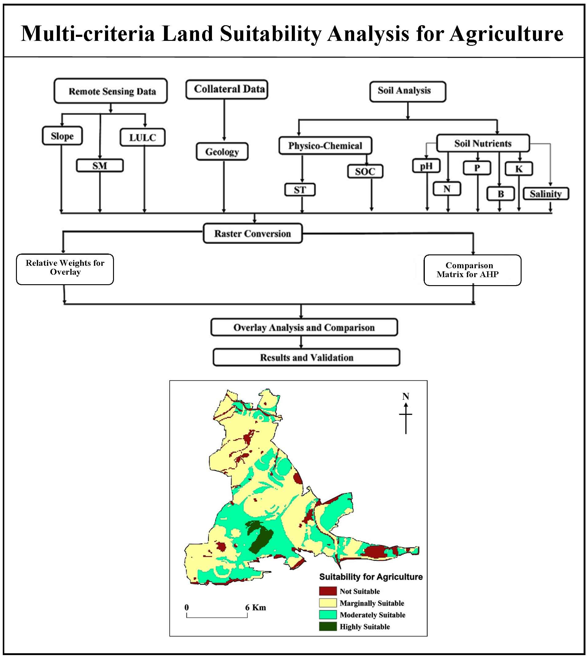
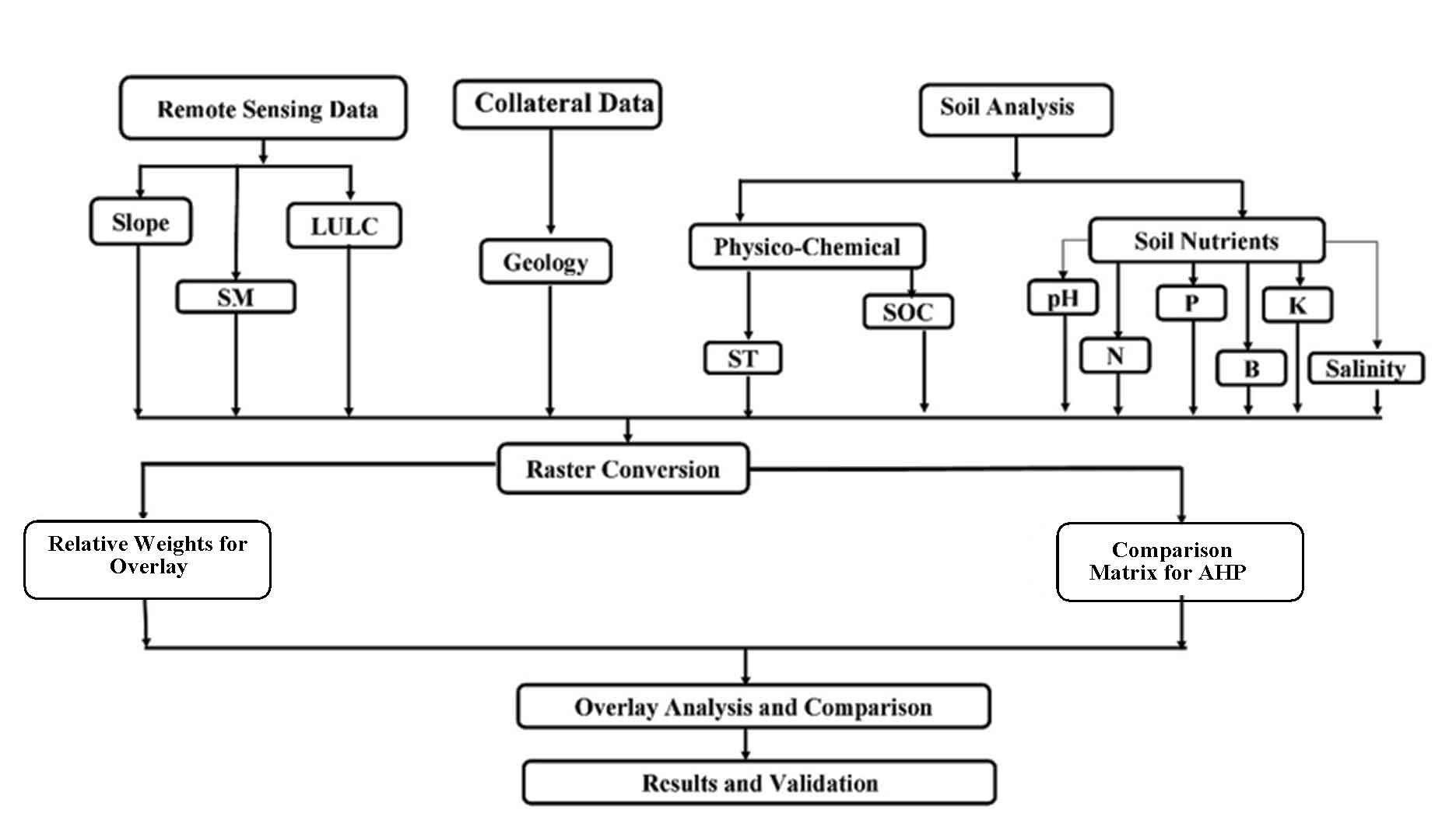
The spatial data concerning chosen criterion i.e.  LULC, soil moisture (SM), soil types, geology, slope, and soil qualities organic carbon (OC), potential of hydrogen (pH), boron (B), nitrogen (N), phosphorus (P), potassium (K), salinity and major nutrients were used. Thematic layers like LULC and SM were all derived from satellite data. Soil types obtained from Bhoomi portal (NBSSLUP) and geology obtained from collateral data (GSI, 2002).  Catrosat DEM were utilized to prepare slope map, whilst laboratory analysis and interpolation technique were employed to generate soil analyses maps (Figure 2).

Figure 2. Methodology

3.2 Satellite Data

Landsat 8 ETM+ (30 m) and IRS-1D LISS-III (23 m) intermediate resolution satellite data are frequently utilized in LSA to identify prospective agriculture, plantation, irrigation, watershed management, settlement, and industry sites (Bandyopadhyay et al., 2009; Mustafa et al., 2011). However, high-resolution satellite data, such as cloud-free conditions, was obtained and analyzed from the NRSC in Hyderabad, India.

3.3 Field Work

In this study, the collected information on LULC, cropping patterns, soil depth and crop productivity. Soil property analysis is a critical stage in LSA. A total of 24 locations near drilled wells were chosen for soil sample using a random sampling approach. These soil samples were analyzed in the lab to determine their physicochemical properties (Kadam et al., 2020). In addition to these physicochemical soil characteristics, land slopes were considered while assessing and evaluating suitable plantation and agricultural land. The moisture content of the soil has a significant impact on plant development and its spread. Bhagat (2009) emphasized the significance of SM in finding potential agricultural sites.

3.4 Criterion

Physical components are inextricably linked to agricultural productivity and agricultural operations (Kadam et al., 2020). LULC, SM, soil types, and geology, as well as OC, pH, B, N, P, K, and salinity, are widely used to evaluate the land’s attributes and suitability for agriculture (Table 3). These parameters have varying degrees of influence and affluence depending on the geographical features. As a result, all criteria were chosen for LSA by WOA (Parry et al., 2018).

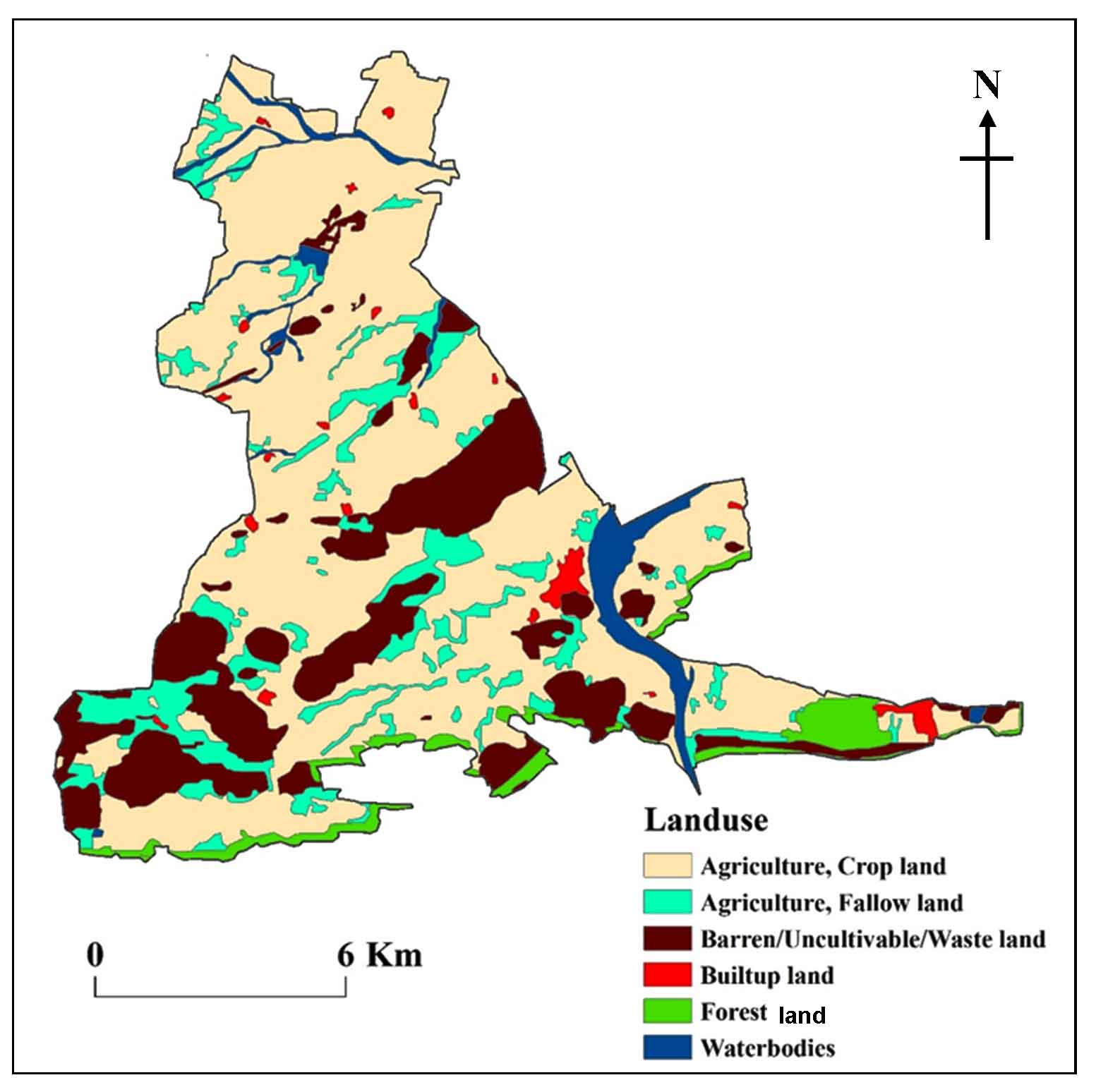
3.4.1 Land use/Land cover (LULC)

We do a qualitative analysis on an image with color composition and enhancement techniques. Analyzing and correlating the item’s spectral signature to the object itself (Prakash, 2003). Satellite sensors provide coverage for reflectance curves of spectrum objects (Rajasekhar et al., 2018) (Figure 3). The spectral signature of soil and plants is subject to changes, such as moisture and plant state (Kumar et al., 2019). Various satellite imageries have been utilized for LULC mapping. Generally, the spectral signature of an object is represented by specific reflectance curves in the portion of the sun spectrum covered by satellite sensors (Tseganeh et al., 2008) (e.g., ick Bird, LISS - IV, LISS - III and Landsat - ETM Soil and vegetation spectral signatures like other objects, change with factors such as wetness and vegetation condition (Nisar Ahamed et al., 2000). A variety of satellite images have been utilized for the LULC mapping. The land use represents the way a piece of land is used, such as for irrigation, agriculture, or housing. Land use is interpretable by satellite imageries (Rajasekhar et al., 2017). Land use examples, such as forest, agriculture, fallow land, barren land, and water bodies are studied in the current study.

Figure 3. Land use land cover

3.4.2 Soil Moisture (SM)

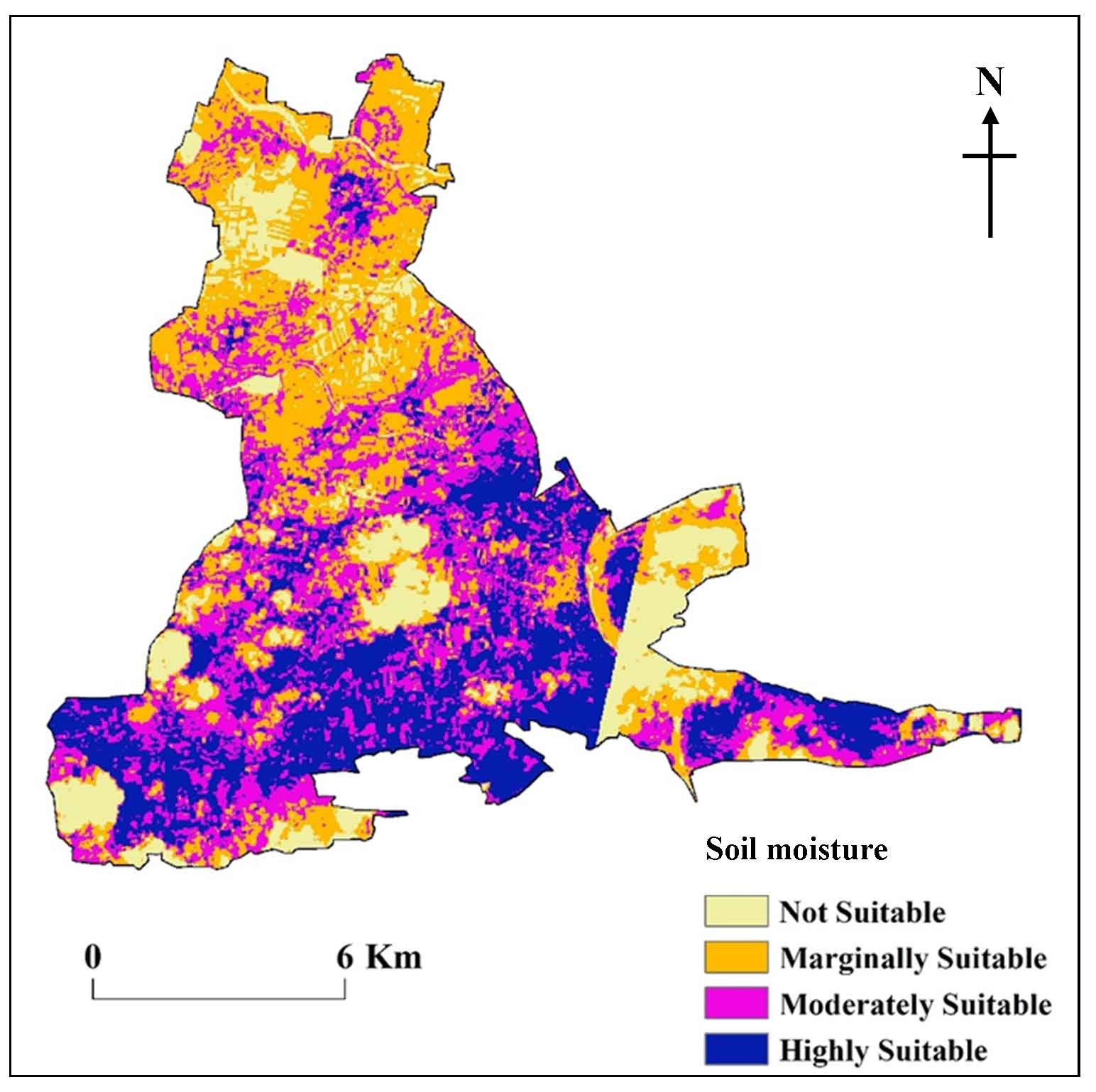
Land’s spectral reflectance varies according to its characteristics, which include soils, rocks, water bodies, plant cover, and built-up area, among others. Water has a lower spectral reflectance than other surfaces (Kumar et al., 2020). The fact that wet soils look darker in SWI images, as well as in others, means that it is more difficult to locate water bodies and soil moisture in SWI and NDVI images (Bhagat and Sonawane, 2011). SM is a good indicator of soil properties and has a favorable association with crop output (Bhagat, 2009; Wang et al., 2012). SM is classified into four categories to identify LSA of the study area (Table 3). Dense forest with deep soils is considered ‘high SM’ for agricultural, fallow, and sparse forests (Figure 4).

Figure 4. Soil moisture

3.4.3 Soil types

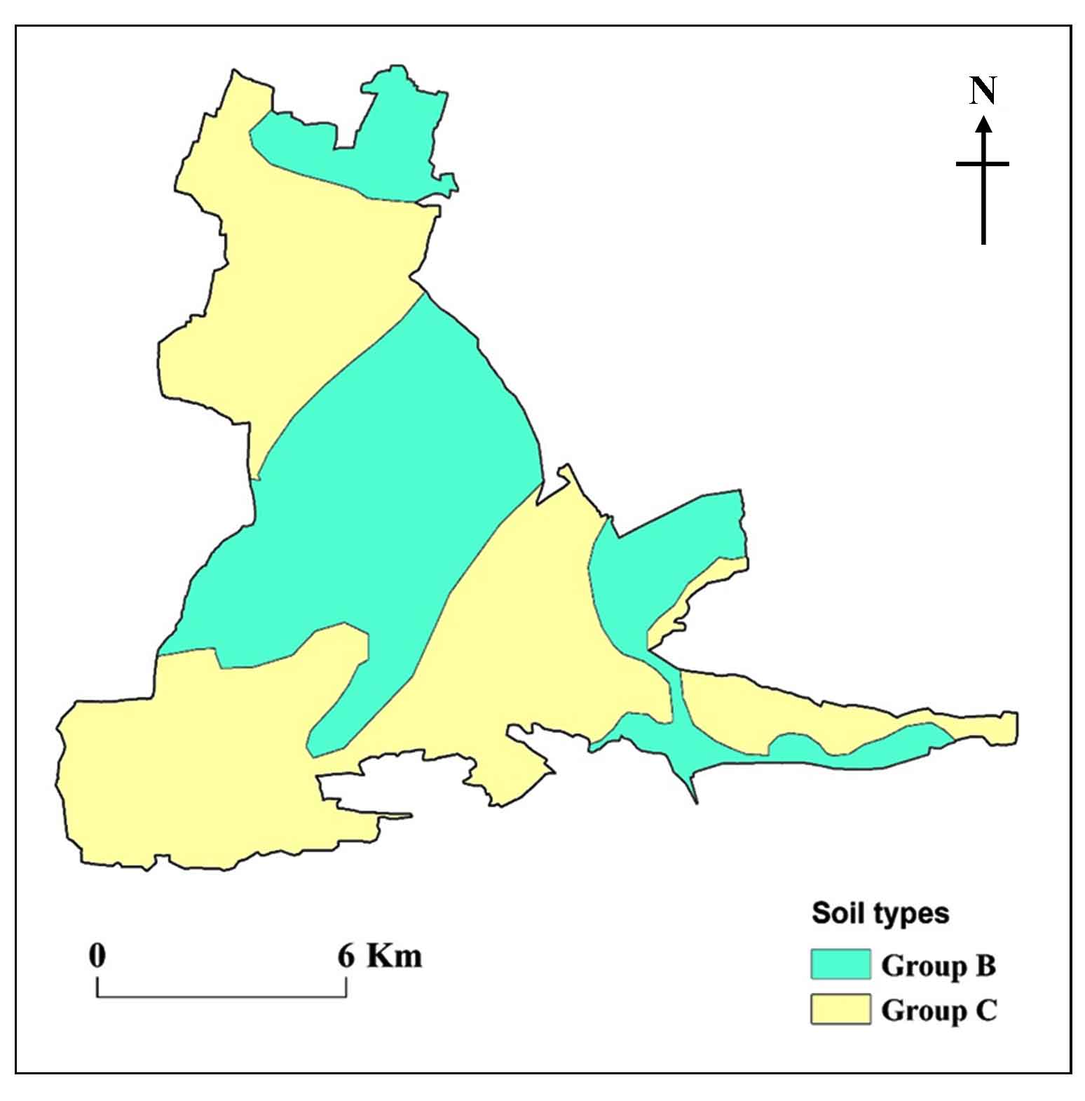
Soils are most important in the LSA based upon their irrigation. These soils are classified into four types based on infiltration rate they are HSG A, B, C and D. Soils heavily containing clay have low moisture condition leads to marginally suitable for agriculture. The sandy soil allows high infiltration results to high moisture condition leads to highly suitable for agriculture (Rajasekhar et al., 2020). The HSGs soil groups of study areas classified as B and C classes are instigated in the present study (Figure 5).  The HSG B soils are in the central part of the region and an area of 69.64 km² (41.40%), HSG C occurs in the southwestern and northern parts of the study region and an area of 98.57 km² (58.60%). The HSG B soils have a higher infiltration rate as compared to the HSG C and HSG B soils high amount SM results highly suitable for LSA.

Figure 5. Soils

3.4.4 Geology

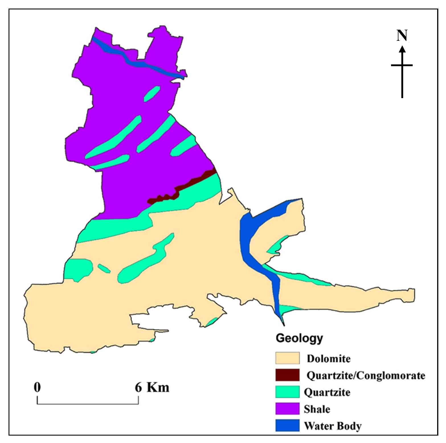
The geological formation of this area incorporates dolomites, quartzites, conglomerates, and shales. It is seen that the study region is commonly composed of quartzites overlain by shales in the major parts of the region. The shales are a low degree of infiltration due to their porosity and permeability nature, while the dolomites formations have a high degree of infiltration due to their permeable nature (GSI, 2002). The quartzites formation of the present study has moderate recharge zones as their nature of the impact, which indicates moderate suitable for agriculture in the present study and dolomites having high filtration factor results highly suitable for agriculture and other hand shale have low degree of infiltration results not suitable for the agriculture in the study area (Figure  6).

Figure 6. Geology

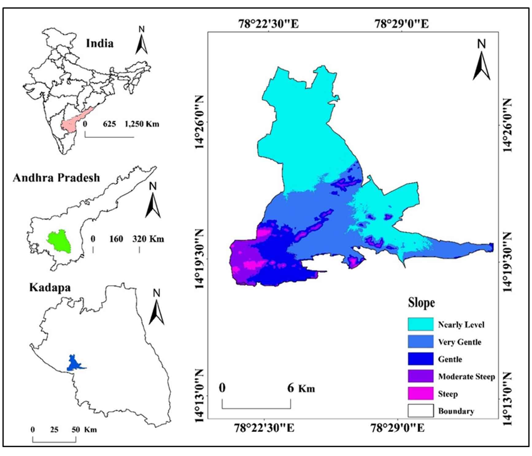
3.4.5 Slope

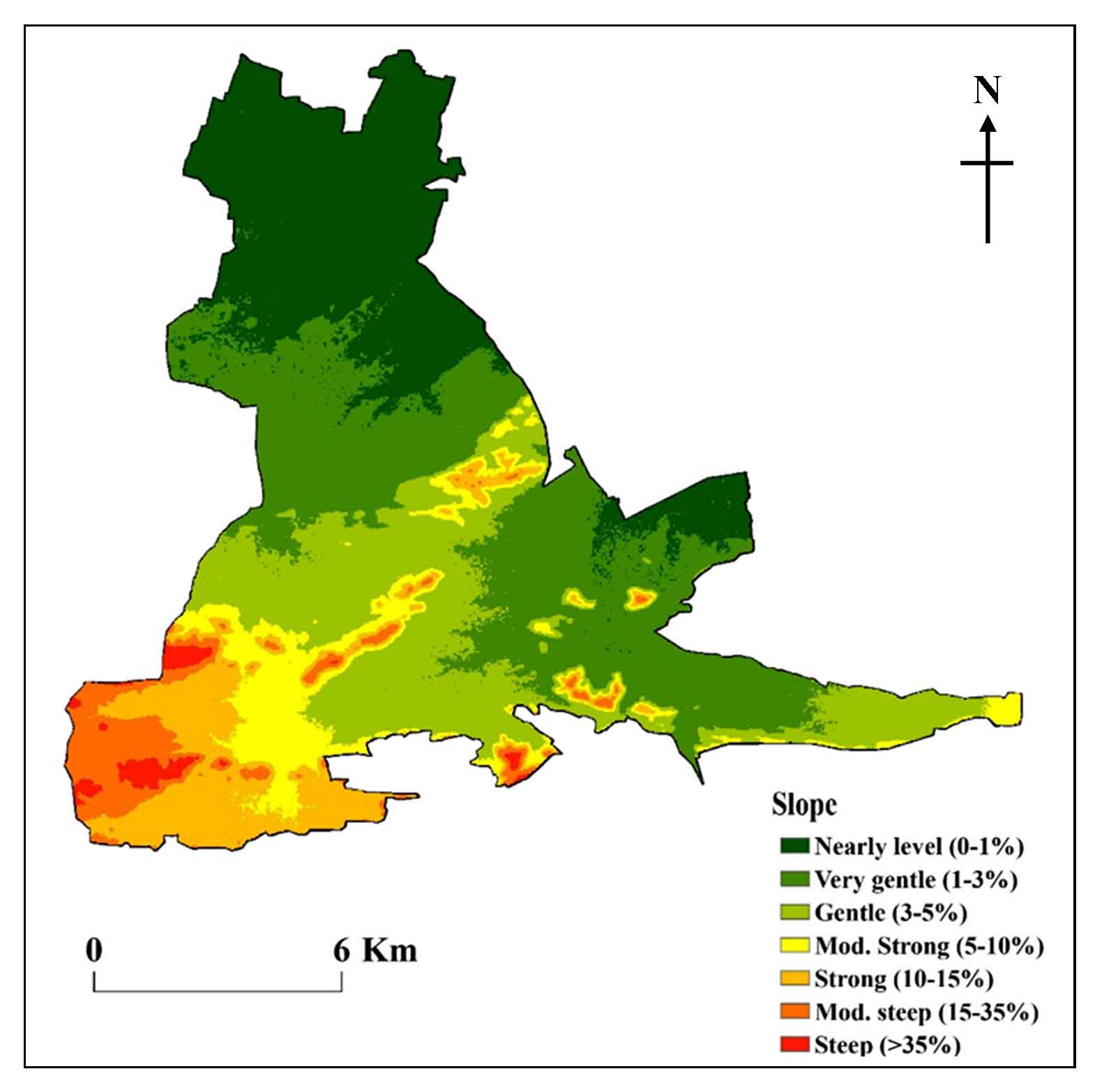
Soil humidity varies because of elevation-based slope. Appreciating the value of LSA for agriculture requires looking at the % slope and the direction of water accumulation (Olshevsky, 2008). IMSD standard describes a seven-level categorization system for percent slopes (IMSD, 1995). The level 0-1 percent region is large storage land with a fairly flat terrain and minimal surface flow. The low-runoff portion, with extremely good water infiltration, has a moderate slope of 1-3 percent. As a result, the infiltration in the water region is quite modest, with a slope of 3-5 percent. The region with a slope of 10-15 percent, moderate soil depth, and high surface flow has less water penetration and thus great for tree planting (Figure 4). The regions with slopes of 15-35 percent are critical for afforestation to help slow soil erosion and replenish groundwater (Table 3; Figure 7).

Figure 7. Slope

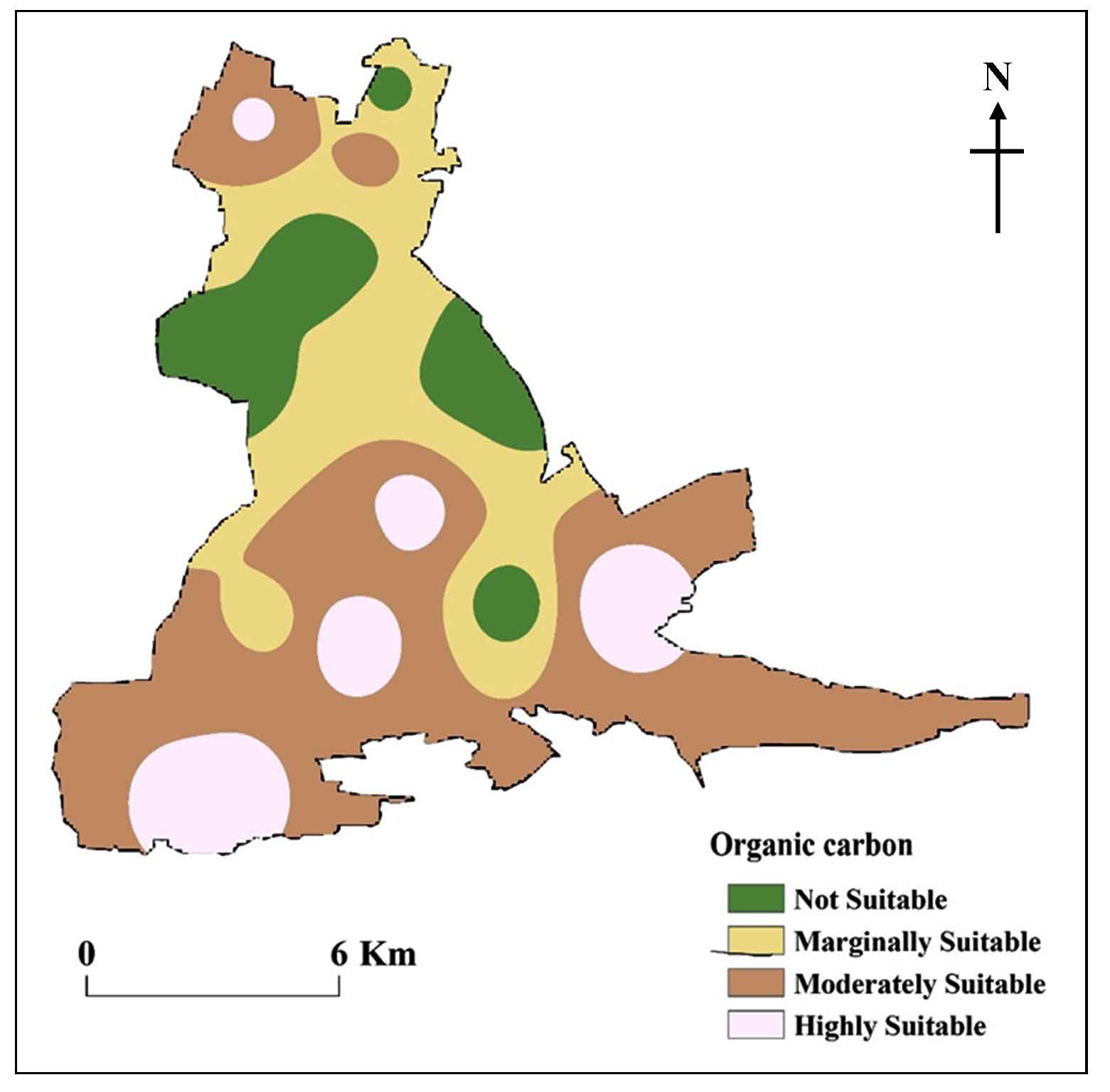
3.4.6 Soil Organic Carbon (SOC)

The SOC is critical for soil fertility, complicated water and nutrient exchange processes in the root zone, and the deterioration of land (Bhagat, 2013). In general, a high organic matter concentration in the soil results in effective mineral fertilizer application. Agriculture and plant life in the downstream zone are harmed by SOC losses (Bhagat, 2013). SOC inhibits soil nutrient build-up and plant development. Soil organic matter varies according to natural soil quality and treatment practices. It was created using laboratory data and interpolation with IDW (Figure 8). More elevations, steep slopes, and higher rainfall exhibit relatively less SOC.

Figure 8. Soil organic carbon

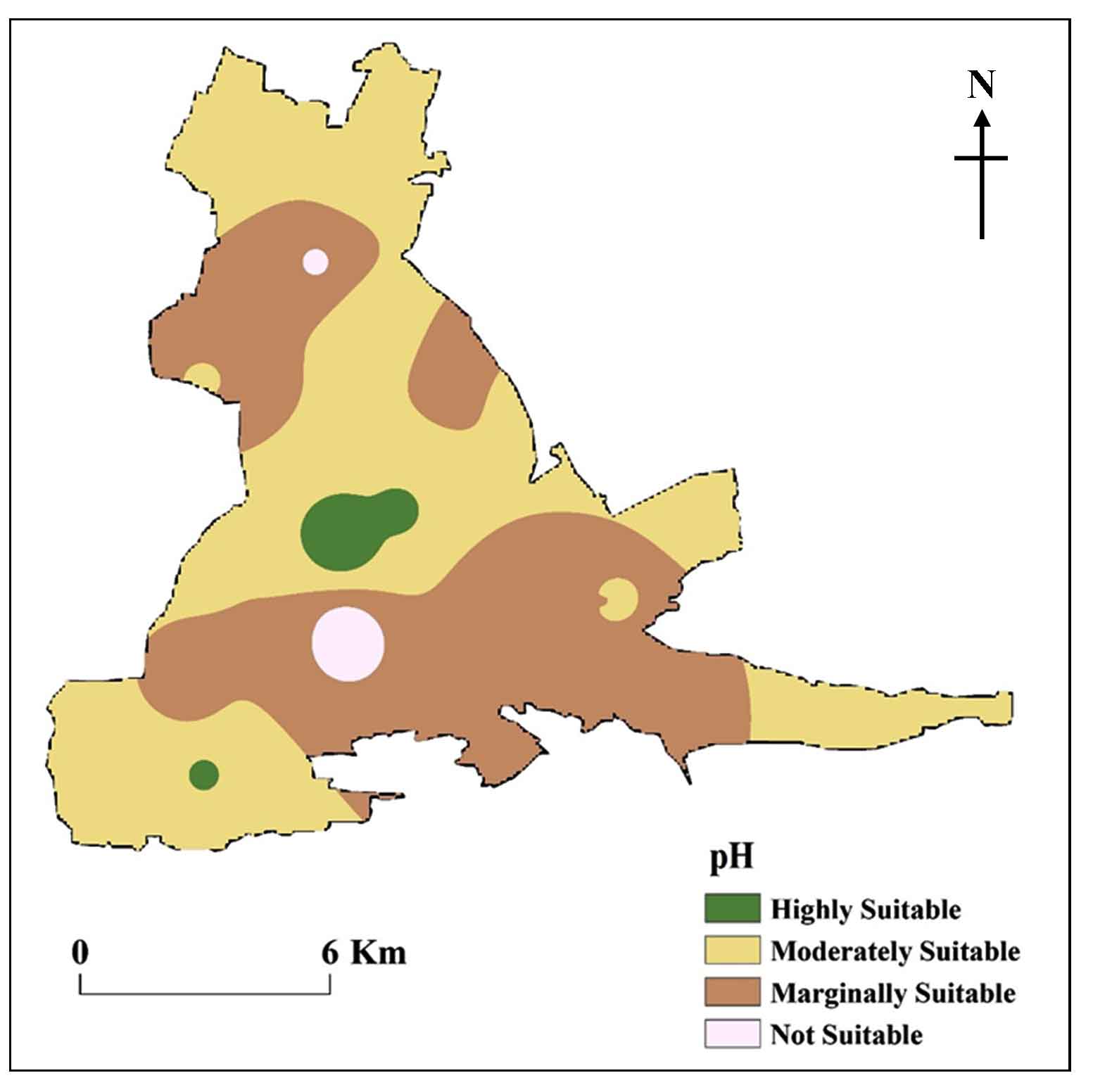
3.4.7 Potential of Hydrogen (pH)

Soil pH is greatly influencing nutrient availability, plant growth, and productivity (Kahsay et al., 2018). The availability of nutrients and phytotoxicity is indicated by the pH of the soil (Tseganeh et al., 2008). pH < 7 is acidic while > 7 is alkaline. However, many plants prefer a pH between 5.5 and 7.0. The pH levels vary between 5.7 and 7.8 pH is typically 6.5, with broad agricultural and plantation applications (Figure  9).

Figure 9. pH

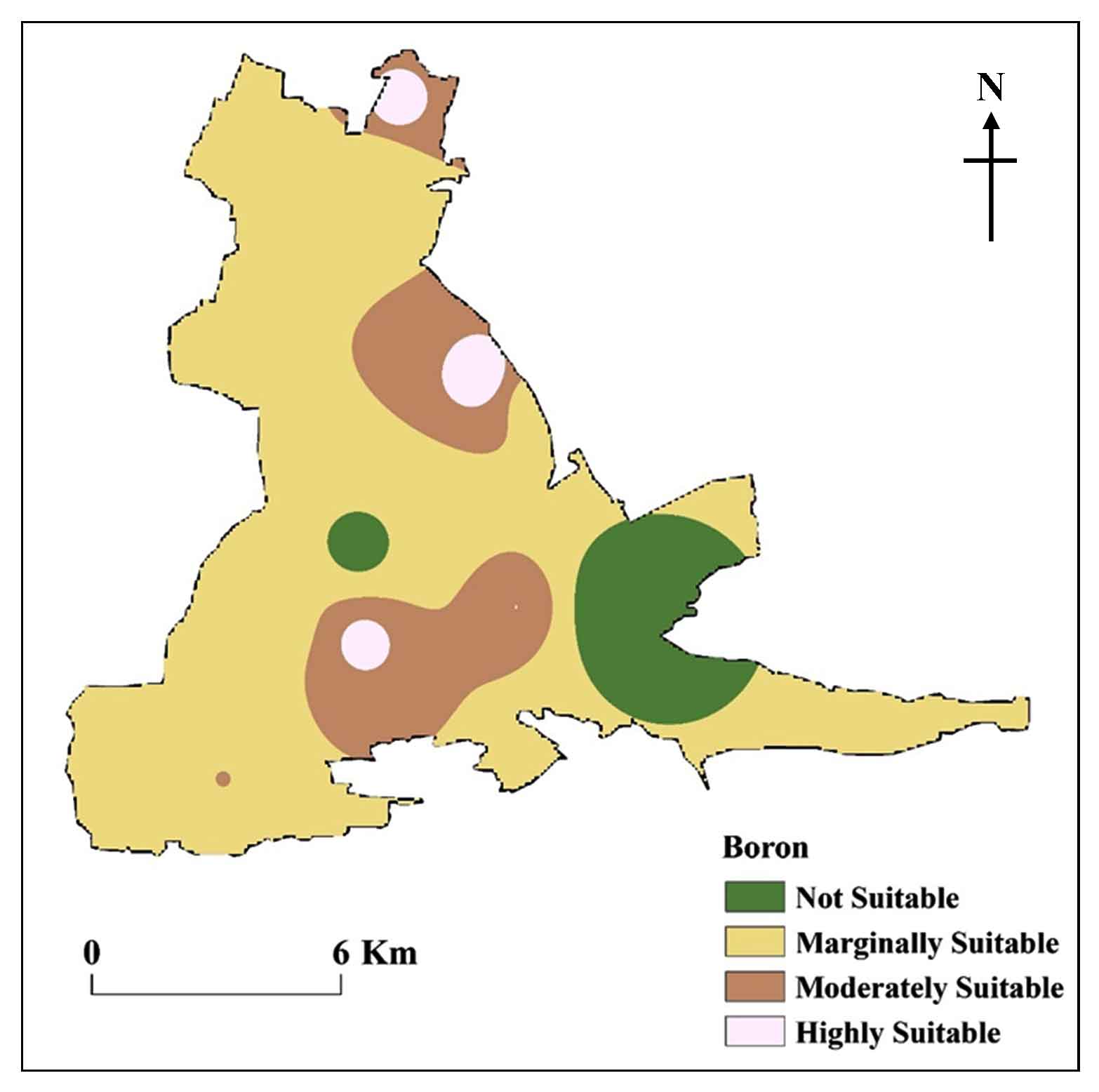
3.4.8 Boron (B)

The critical B requirement for different plant species differs, with monocots (wheat, barley, etc.) requiring 5-10 mg/kg DM and dicots (legumes) needing 20-70 mg/kg  (Ennaji et al., 2018). Pectin is found in all plants; however, levels are different in monocots and dicots. Monocots have substantially lower Ca needs, but they also have less pectic material in their cell walls. Administration of both Ca and B to four maize cultivars considerably increased dry matter output (Kanwal et al., 2008). Toxicity limits for excess B are: 100-270 for wheat 400 for cucumber, and 100 for squash. Crop sensitivity to B deficiency and toxicity differs (Figure 10).

Figure 10. Boron

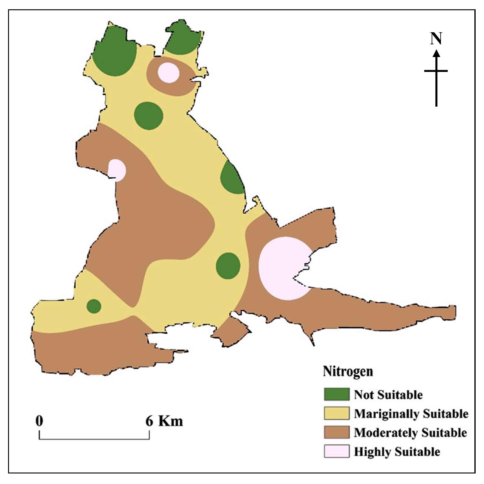
3.4.9 Nitrogen (N)

Plant growth depends on the presence of nitrogen (Mustafa et al., 2011). N concentrations in the soil are estimated using samples collected from the study region. GIS layer showing N has values set with IDW interpolation technique in GIS. Water soluble nitrogen was leached from our research region during intense rainfall (Figure 11).

Figure 11. Nitrogen

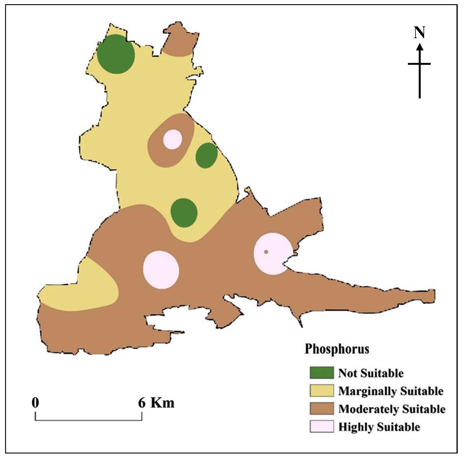
3.4.10 Phosphorus (P)

Phosphorus is required for a variety of activities, including root development and growth, crop maturity, blooming, and seed generation, among others. Acidic or alkaline soils required a higher concentration of phosphorus for optimum plant development. Because of this, P is identified and quantified in the laboratory and then applied to LSA results. Using this data, it is determined that the region is just moderately appropriate for agriculture, with a maximum value of 46.1 kg/ha and a minimum value of 7.8 kg/ha, and an average value of 16.24 kg/ha (Figure 12).

Figure 12. Phosphorus

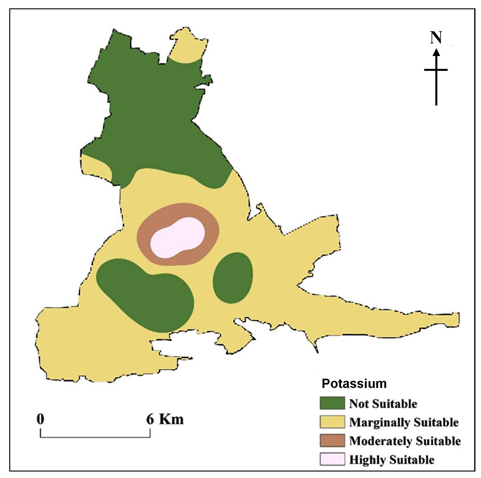
3.4.11 Potassium (K)

For a variety of plant functions to occur, potassium is required, including (1) photosynthetic activity, (2) stalk and stem stiffness, (3) disease resistance, (4) drought tolerance, (5) grain and seed plumpness, (6) fruit hardness and texture, as well as size, color, and size distribution, and (7) oil content in oil seeds. Due to a lack of potash, the plant’s green color fades to yellow, and its lower leaves disappear, resulting in a reduction in production (Figure 13).

Figure 13. Potassium

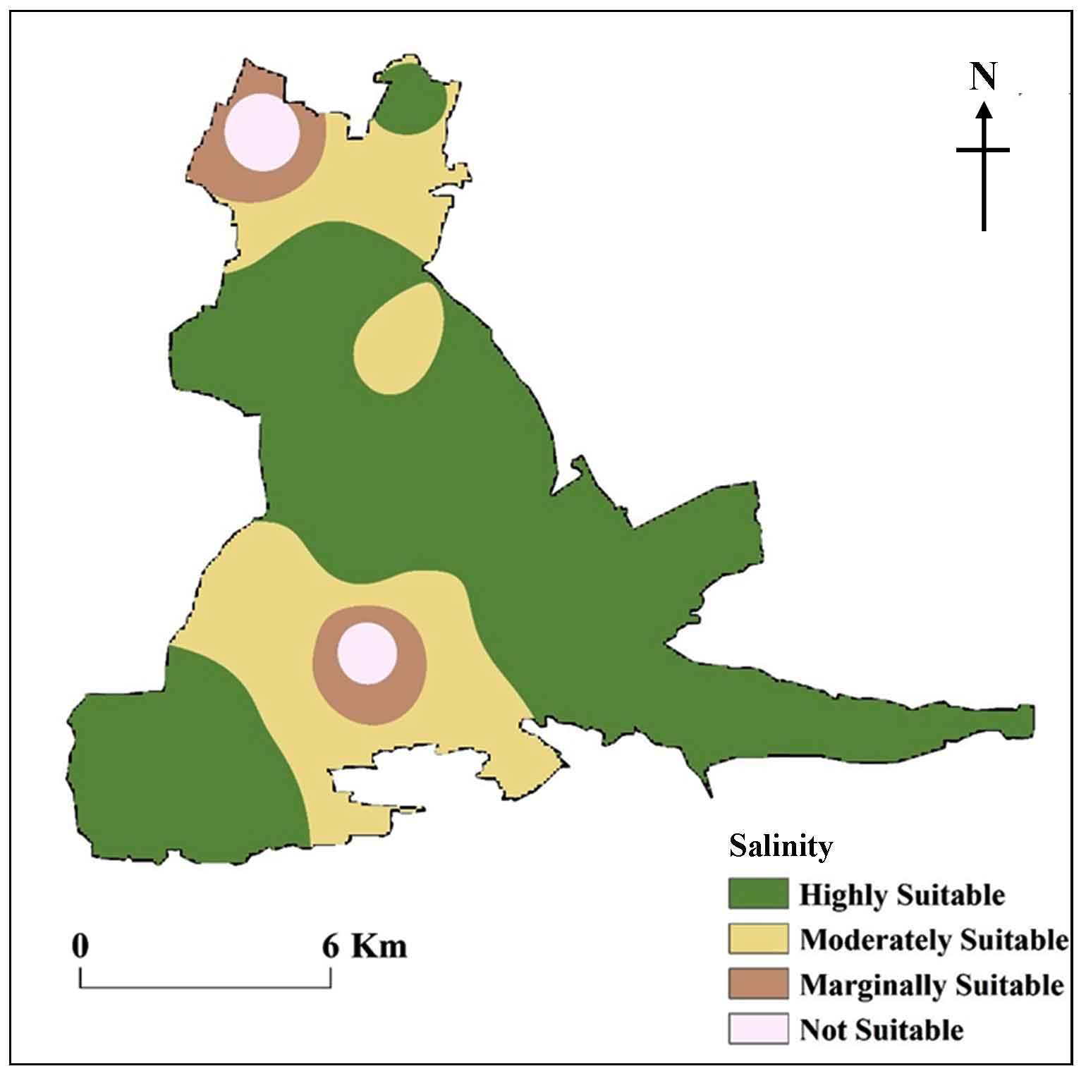
3.4.12 Salinity

These general problems are low agricultural intensity, water shortage, and poor crop yield and soil salinity. These could be dealt with by using management measures such as crop diversification that uses less water-using crops and drainage maintenance to combat soil salinity. However, if farmers are mobilized, if researchers are flexible, and if the farmers have their say, collaborating and experimenting with farmers could lead to success (Ennaji et al., 2018). According to the predicted yield function, seed variety, administration of appropriate doses of weedicides, sowing dates, irrigation application, and groundwater quality were significant contributors to yield discrepancies (Figure 14).

Figure 14. Salinity

3.5 Assigning the Weights by AHP

The AHP simplifies the parameters of the PCM and is dependent on the assigning of experts concerning the significance of the influencing factors. AHP is one of the most common approaches in decision making analysis (Saaty, 1980, 1990 and 2008; Kadam et al., 2017; Shailaja et al., 2018). This process also can analyse proportionally various datasets through the PCM analysis of each parameter and flexibility in the situation of intentions (Rajasekhar, 2019; Shailaja et al., 2018). Saaty (1980) initially carried out this systematic exercise to show sustainability and the consequences in a multilateral decision-making system. The matrix structure of AHP offers the possibility to quantify and synthesize different features of the multi-lateral decision making process hierarchically.

In this analysis, AHP is used to estimate the weight of all related parameters concerning groundwater recharge capacity in the research area (Table 4). AHP implies an assessment of the significance between the parameters, the normalization and calculating the consistency ratio (CR). Depending on the hierarchical order constructed, it is decided that the priority of the influencing factors recognizes the significance of the features at various levels of the hierarchy (Mustafa et al., 2011; Das, 2019; Kaliraj et al., 2014). To obtain qualitative data, the factors that influence each level are compared in pairs. The Saaty scale from 1 to 9 (Table 1) is used to measure the relative importance of the factor (Saaty, 2008).

3.6 Pairwise Comparison Matrix (PCM)

This prepares a diagonal matrix by placing values in the upper triangle and using their reciprocal values to fill the triangular matrix. The expert’s judgment was used for PCM (Zolekar and Bhagat, 2015). Also, the relative weights were normalized. The normalized principal eigenvector is obtained by averaging the order to verify the consistency of the priority vector. The key own value is acquired by applying the products to each part of the own vector and summing the columns of Table 2 and Table 3. This fundamental eigenvalue is used to degree the consistency of ideas through an analysis of the consistency ratio (CR) (Saaty, 1980). A CR value lesser than 0.1 can be considered as opinion with less uncertainty in weight determination (Kadam et al., 2018). The Consistency Index (CI) is calculated using the below equations and the comparison matrix to compare all parameters for calculating CR.

\(CI = {{\lambda max - n} \over n - 1}\)              (1)

where, λmax is consistency vector and n is number of criteria or factors

The CR has been calculated based on equation 2.

\(CR = {{CI} \over RCI}\)                  (2)

where, RCI is random consistency index, provided by Saaty (2008)  (Table 1).

4 . RESULTS AND DISCUSSIONS

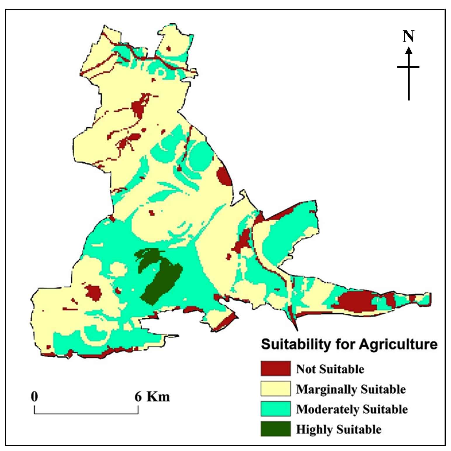
The LSA was mapped using Weighed Overlay Analysis (WOA), with the weights of selected criteria obtained in the AHP analysis and the given scores of sub-criteria serving as the inputs. For agricultural purposes, LSA is classified into four categories: highly suitable, moderately suitable, marginally suitable, and not suitable.

4.1 Highly Suitable

Approximately 2.62 % (4.42 km²) of the land in the study region was assessed as “highly suitable” for agriculture (Figure 15), with 20.12 % of the land under crop production and 15.16 % under fallow land. Slight to moderate slopes, deep loam soils with improved water retention capacity and soil moisture, as well as a pH in the normal range, characterize this land type (Table 4). If enough irrigation infrastructure and financial support are available, the fallow lands categorized in this category can be converted into productive agricultural regions. The minor limitations in these locations include low to moderate soil nutrients such as nitrogen, phosphorus, and potassium, which necessitate the use of external inputs in order to achieve optimal agricultural production.

Figure 15. Land suitability for agriculture

4.2 Moderately Suitable

According to the results of the study, about 32.33 % (54.39 km²) of the sites were rated “moderately suitable” for agriculture (Figure 15). These areas are characterized by steep slopes, loam soil with a modest depth, water retention capacity, soil wetness, and erosion resistance (Table 4). These regions are fallow lands, overgrown with grasses, and devoid of trees, necessitating the use of additional inputs as well as the application of intensive farm management techniques for agriculture.

4.3 Marginally Suitable

On the whole, 56.93 % of the study region (95.76 km²) is classified as “marginally suitable” (Table 4; Figure 15). This class show shallow soils with steep slopes, limited water retention capacity, decreased soil moisture and nutrients, and higher erosion rates than other types of fields. Moderately steep slopes are frequently overlooked while planning agricultural operations. Some of the steep slopes with deep soils and abundance of rainfall may be terraced and utilized to grow crops like as paddy, groundnuts, and Bengal gram, among others, while others are left uncultivated. Extreme soil erosion must be avoided in these fields at all costs.

4.4 Not Suitable

Steep slopes with rocky surfaces, barrenness, thin and dry soils, and other factors that make them unsuitable for cultivation account for 8.11 % (13.64 km²) of all agricultural land (Table 4 and Figure 15). The study area is in the eastern portion of the research area and has been designated as an environmentally fragile zone that must be protected and maintained at all costs. It follows as a result that agricultural operations are forbidden on medium to dense forest lands, as well as on urbanized areas.

5 . CONCLUSION

The overall objective of this study was to discover agricultural land in Kadapa district that would be lost to semi-arid zones and to find alternative fields using RS, GIS and AHP techniques. These analyses used 12 factors to reflect the geographic and soil features of the region. At the completion of the evaluation, just 2.62% of the research area was found highly suitable for agricultural production. It was found that poor agricultural land availability is attributable to two main causes. The first, and most effective, is that a considerable portion of arable land is adjacent to forest and grazing areas. To protect forest and pasture lands, the Kadapa ordinance restricts their use for any other purpose, including agricultural cultivation. The second cause is a compilation of issues arising from the study area’s geomorphological characteristics. Except for their slightly acidic qualities, the brown forest soils that comprise the study area’s dominating great soil group have no adverse effects on agricultural productivity. Additionally, the area’s alluvial soils are suited for agricultural development. Furthermore, the existing environment and the agricultural products that are now being cultivated indicate that Kadapa’s agricultural output potential is enormous. In a contrast, topographical issues, such as a steep slope, have a negative impact on the degree of erosion, the pace of bare rock formation, the depth of soil, and the land use capacity class of the area. The combination of all these factors resulted in the study region having a very small quantity of land highly suitable for agricultural growth.

Tables

Figures

Conflict of Interest

Acknowledgements

Abbreviations

References