Keywords

Sediment Texture , Sedimentology , Monsoon Variability , Magnetic Susceptibility , Grain-size

1 . INTRODUCTION

The study of palaeomonsoon is essential for human being because life of the people is directly or indirectly depend on the climate i.e. rainfall and temperature. The study of past monsoon in India is very significant because around 80% of rainfall received from southwest summer monsoon. All the agricultural and other human originated activities are depending on monsoon and all hydrologic systems on the Earth operated according to changes in the precipitation. A minor variation in the rainfall cause severe droughts and floods and it can adversely affect the agriculture and human being causing migration of people (Gupta and Thamban, 2008). Therefore, it becomes necessary to investigate the past rainfall variability. With the help of reconstruction of past climate (monsoon), we can infer about future behavior of rainfall and can take some precautions to adopt the future climatic variability in advance. Palaeoclimatic observations are useful in building of climatic models.

The investigation of the fluvial deposits in the small catchments proved valuable while studying variations of the river activity in response to the climatic changes. The work and characteristics of the river with large catchment area affected by more geo-environmental factors, such as weathering, erosion, lithology, tectonic activity, climate change, base level changes, etc. Therefore, due to factors involved in the process of work of large river are more, the investigation of fluvial deposition become very complicated and it also becomes difficult to determine dominant factor(s) leading to deposition and the source of sediments (Brown, 2003).

The fluvial deposition has not preserved for long period. Due to high-energy flows, the sediment records of the rivers often destroyed. Hence, continuous past climatic changes in the catchment has not understood. In this regard, tanks located in the foothill zones are very significant, as they are least affected by post depositional changes and preserves the continuous records of palaeoenvironmental changes spanning a few decades to a few thousand years.

The study of the grain-size distribution, mineral magnetic studies and other sedimentological characteristics of the tank sediments preserved in the foothill zones can provide valuable information on the hydrodynamic conditions prevailing on the hill-slopes and the catchment area at the time of deposition (Pettijohn, 1975; Collinson and Thompson, 1989).    Tank sediments are well-dated and high-resolution archives on the continents. It is very responsive to climatic and hydrological changes therefore, it can be used to reconstruct palaeomonsoon variability by studying multi-proxies such as sedimentology, mineralogy, geochemistry, etc. (Kotlia et al., 2010).

Due to high potential of lacustrine deposits for palaeoclimatic reconstructions, from India several workers have been carried out investigations on the lacustrine deposits during last two to three decades (Kale et al., 2003). Many studies on environmental change in India are based on lacustrine deposits in the Himalaya and Western India including the study of Tsokar Tank in Ladakh (Bhattacharyya, 1989), Manasbal Tank in Kashmir (Kusumgar et al., 1992), Sitikher Bog in Himachal Pradesh (Chauhan et al., 2000), Lunkaransar and Sambar Tank in Rajasthan (Enzel et al., 1999; Sinha et al., 2004), Nal Sarovar in Gujarat (Prasad et al., 1997),  Goting tank in Garhwal (Ghosh et al., 2003), Proglacial tank in central Himalaya (Basavaiah et al., 2004),  Phulara tank in Kumaun Himalaya (Kotlia et al., 2010), Bap-Malar and Kanod playa in Thar desert (Deotare et al., 2004), etc. A few studies of tank deposits have been undertaken from the Deccan Peninsula (Shankar et al., 2006).

These multi-proxy lacustrine records, along with other terrestrial records (colluvial, alluvial, loess and lagoon deposits, paleosols, speleothem, waterfall tufa, etc.)  from Himalaya (Phadtare, 2000; Pant et al., 2005a, 2005b), Western India (Bryson and Swain, 1981; Singh et al., 1990; Andrews et al., 1998; Enzel et al., 1999; Kale et al., 2000; Juyal et al., 2000;  Kar et al., 2001; Jain and Tandon, 2003; Sant et al., 2004)  and Deccan Peninsula (Joshi and Kale, 1997; Pawar et al., 1988; Sukumar et al., 1993; Sukhija et al., 1998; Yadava and Ramesh, 1999; Yadava et al., 2004; Thomas et al., 2007; Sandeep et al., 2012) indicates the climatic instability over the India and prone to rapid changes during the late Quaternary period.

   From the Deccan Basalt Province, however, no such multi-proxy studies have carried out so far. Therefore, it decided to undertake a study on the tank sediments of historical tank from the sub-humid zone of Western Maharashtra. Tanks located in the foothill zones have proved to be valuable in this regard; because they are least affected by post-depositional changes and even smaller variation in the rainfall condition can be well preserved in the tank sediments. Therefore, Vaghad Tank located in the Nashik district of Western Maharashtra was studied. We reasoned that this historical tank may provide interesting information about the past monsoon conditions prevailed in the catchment area. Therefore, the main objctive of present paper is to study the sedimentary deposits of  the Vaghad Tank to understand the past monsoon variability prevailed during the deposition of the sediments.

2 . STUDY AREA: VAGHAD TANK

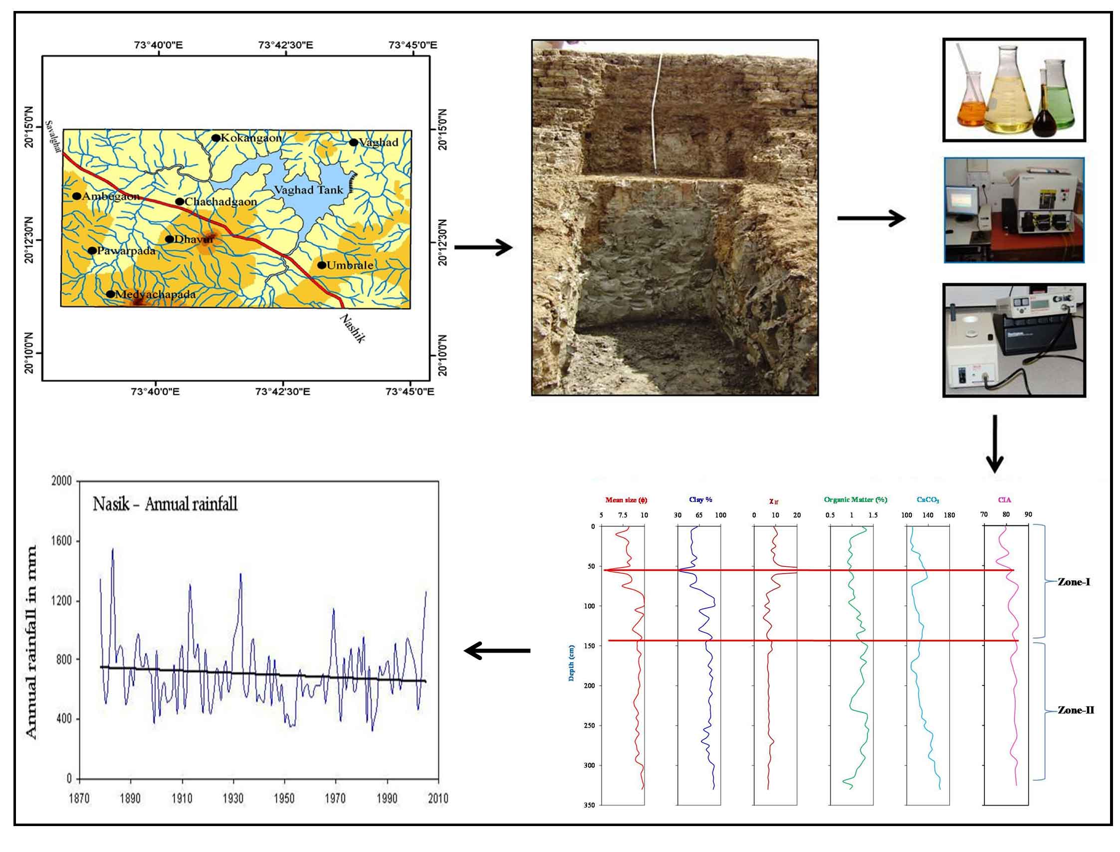
The Vaghad Tank (20º 14¢ N and 73º 42¢ E) is located about 25km North of the Nashik City, on the Nashik-Penth Road (Figure 1).  The catchment area covered by the tank is 74.5km². According to the Gazetteer of Nashik District (1975), the Vaghad Reservoir made in 1878 CE as famine relief work. It means that the tank is about 142 years old. The altitude varies between 640 and 953 m ASL. This is the historical tank located in the sub-humid zone with an annual rainfall exceeding 1000 mm.

Figure 1. Study area: Vaghad Tank, District- Nashik, Maharashtra (India)

In spite of wetter conditions, vegetation cover is completely absent. However, the area around the tank is intensively cultivated. The Kolvan River is the major source of water and sediment flux to the tank. The tank sediments exposed by step-trenching for stratigraphical studies taken at the center. The Chachadgaon, Kokangaon, Vaghad and Umbrale are the main villages located in the neighborhood of the tank (Figure 1).

3 . MATERIALS AND METHODS

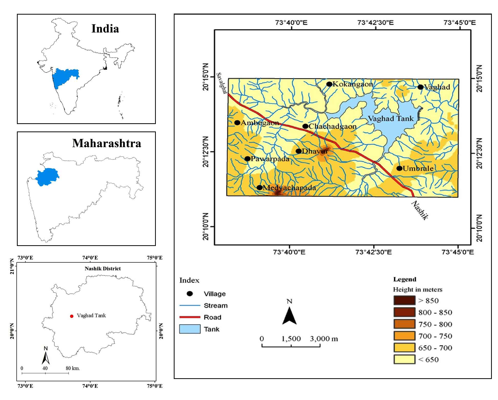
To determine the changes in the stratigraphical and sedimentological characteristics of sediments with different time scale, a 3.3 m step-trench made in the center of the tank (Figure 2).  Detailed stratigraphical studies carried out after exposing the sediments. The sediment color was determined by comparison with the Munsell Soil Color Chart (Munsell Color, 1975). The Miall’s lithocodes (Miall, 1985) applied to each unit to understand the nature of sediments. Total 67 sediment samples were collected at an interval of 5 cm from the exposed lithosection for textural, geochemical and mineral magnetic analyses.

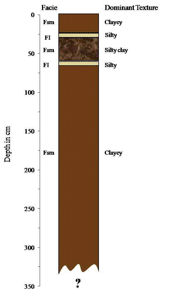
Figure 2. Vertical section of the sedimentary deposits

In the laboratory, for coarse sediments mechanical sieving was performed and for finer fraction, analysis was undertaken using Sedigraph-III Particle Size Analyzer (Operator’s Manual, 2018) to understand grain-size distribution in the sediments. The textural data employed to obtain the percentage of sand, silt and clay. The statistical parameters (mean size, sorting, skewness and kurtosis) were derived by applying formulae given by Folk and Ward (1957).

Magnetic susceptibility analysis performed on the bulk sediment samples using Bartington MS2B magnetic susceptibility meter with a dual-frequency sensor operating at low and high frequency magnetic susceptibility (0.47 kHz and 4.7 kHz) and an AGICO’s KLY-2 Kappabridge susceptibility meter. The rock magnetic parameters, low frequency mass specific magnetic susceptibility and its frequency dependent component, were calculated from low-frequency and high-frequency measurements to get some idea about the concentration and grain-size distribution of magnetic minerals following Basavaiah and Khadkikar (2004) and  Foster et al. (2008).

Low frequency mass Specific magnetic susceptibility (\(X_{if} \)) (Equation 1) and frequency dependent susceptibility ( \(X_{fd}\) ) (Equation 2) calculated as:

\(X_{if} = (X_{LF} \times 10^{-10}m^3/(g \times10^{-3}kg\)      (1)

\(X_{fd}\)(%)\( = (X_{LF} - X_{HF}/X_{LF}) \times 100\)       (2)

where, \(X_{if} \)  represents low frequency mass specific magnetic susceptibility, \(X_{LF} \)  represents susceptibility values measured at 0.47 kHz and ‘g’ shows the weight of sediment sample in grams. \(X_{fd}\)(%) represents percentage frequency dependent susceptibility and \(X_{HF} \)  represents susceptibility values measured 4.7 kHz.    

The content of carbon and organic matter has estimated by back titration with Walkley and Black Method (Walkley and Black, 1934). The following formulas used to calculate percentage of carbon and percentage of organic matter:

C (%) =  3.951/g (1- T/S)                                    (3)

Organic matter (%) = C(%) * 1.724                 (4)

where, g = weight of sample in gms, S = ml ferrous solution with blank titration, T = ml ferrous solution with sample titration.

The calcium carbonate content for all the samples has estimated by back titration with neutralization method. The following formulas used to determine the percentage of calcium carbonate (CaCO₃) in the sediment samples.

Meq = volume (ml) X  Normality                      (5)                                                   

Meq Calcium carbonate equivalent in 4gms soil = (meq HCL added – meq NaOH used) / (weight of sample (g)) (6)   

The stratigraphical and geochemial data has synthesized to understand the nature of changes in the rainfall condition prevailed in the catchment area of the Vaghad Tank. The rainfall data of Nashik is obtained from the Indian Meteorological Department, Pune and processed in MS Excel to show the trend in average annual and highest daily rainfall for Nashik Station.

4 . RESULTS

4.1 Lithostratigraphical Observations

The total thickness of the lithosection was about 3.3 m (Figure 3). It comprising about 10 minor stratigraphical units but based on color, texture and bounding surface of the sediments, only five major units of sediments observed. Figure 3 shows the stratigraphy of the sediment section observed during fieldwork and the actual photograph of litho-section (Figure 2).

The measured thickness of the individual layer ranges between 5 and 90 cm. In general, most units featured by high clay content. Silt units observed at 30 and 65 cm depth. A very thin silt layer (~5 cm thick) is present in the upper part of the section. Field investigations revealed alternative bands of clay and silt found up to the depth of 65 cm from the top and below which clay dominates all the units (Figure 2 and Figure 3).

Figure 3. Litho-stratigraphic section

All the sediment units display massive internal structure and alternate sharp and gradual bounding surfaces, indicating variations in the energy of flow. The upper sedimentary units were brown to dark brown in color. The sedimentary unit at the step displays reddish coating and the bottom unit is dark black in color (Figure 2).

4.2 Textural Characteristics

The textural data (Table 1) concludes that the tank sediments dominated by clay. The average of clay is roughly 75%. Vertically, the clay ranges between 30.3 and 89.6%. These samples contain a very low proportion of sand between 0 and 26.3%. The average sand content is 0.73%. The silt comprises about 24.3% and silt in the samples ranges from 7 to 48.2%. Thus, deposit in Vaghad Tank dominated by very fine particles.

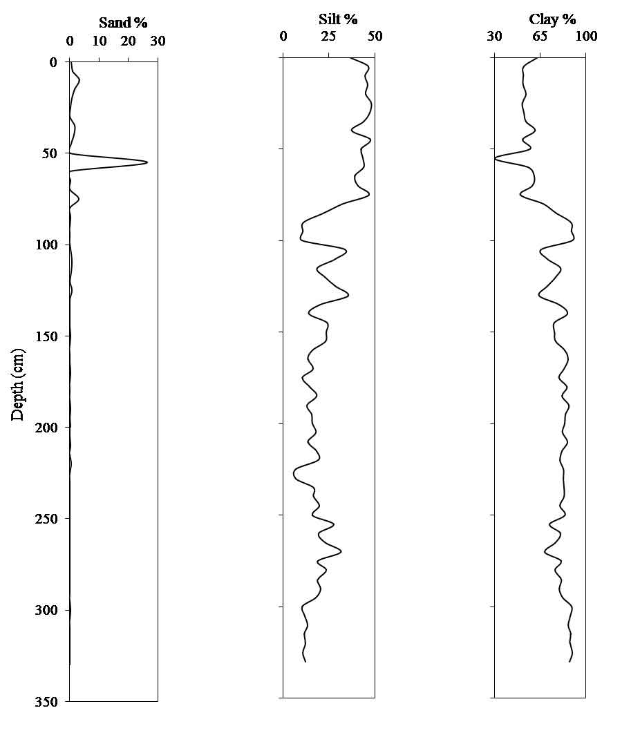
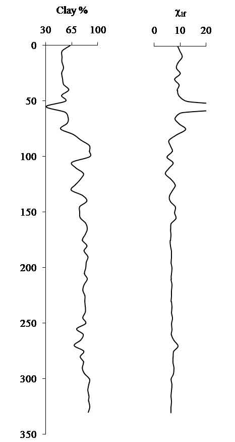
The vertical variation in the textural classes shows an upward coarsening sequence (Figure 4). The upper units are slightly coarser than the lower units. Only one unit occurring at 55 cm from the top, has a high percentage of sand (26.3%) and low percentage of clay (30.3%) as compared to the other units (Figure 4). Highest concentration of clay is observed at the level of 100 cm from the top, which is 89.6% and this level is also characterized by a relatively low percentage of silt (10.4%). The amount of clay increases and silt decreases from top to bottom whereas the percentage of sand exhibits random variation (Figure 4).

Figure 4. Vertical variations in the texture

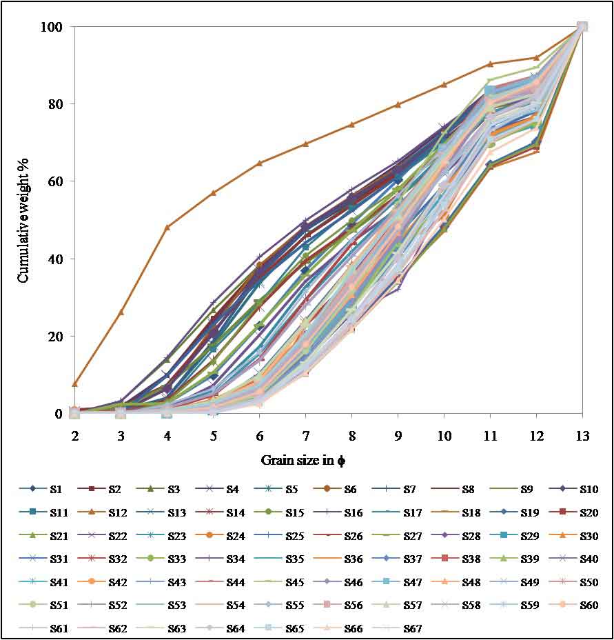
It is evident from the plot that the cumulative grain-size frequency curves for all the samples are identical and there are no major variations in grain-size, except in samples collected from 12 to 55 cm from the top, which shows a sharp deviation in the upward direction from the other curves (Figure 5). The sample number 12 suggests the predominance of coarse material whereas the remaining samples characterized by fine material because they lean towards horizontal axis (Figure 5).  The curves of grain-size distribution indicate, more or less, identical energy condition during deposition.

Figure 5. Plots of cumulative grain-size frequency curves

4.3 Vertical Variation in the Grain-size Parameters

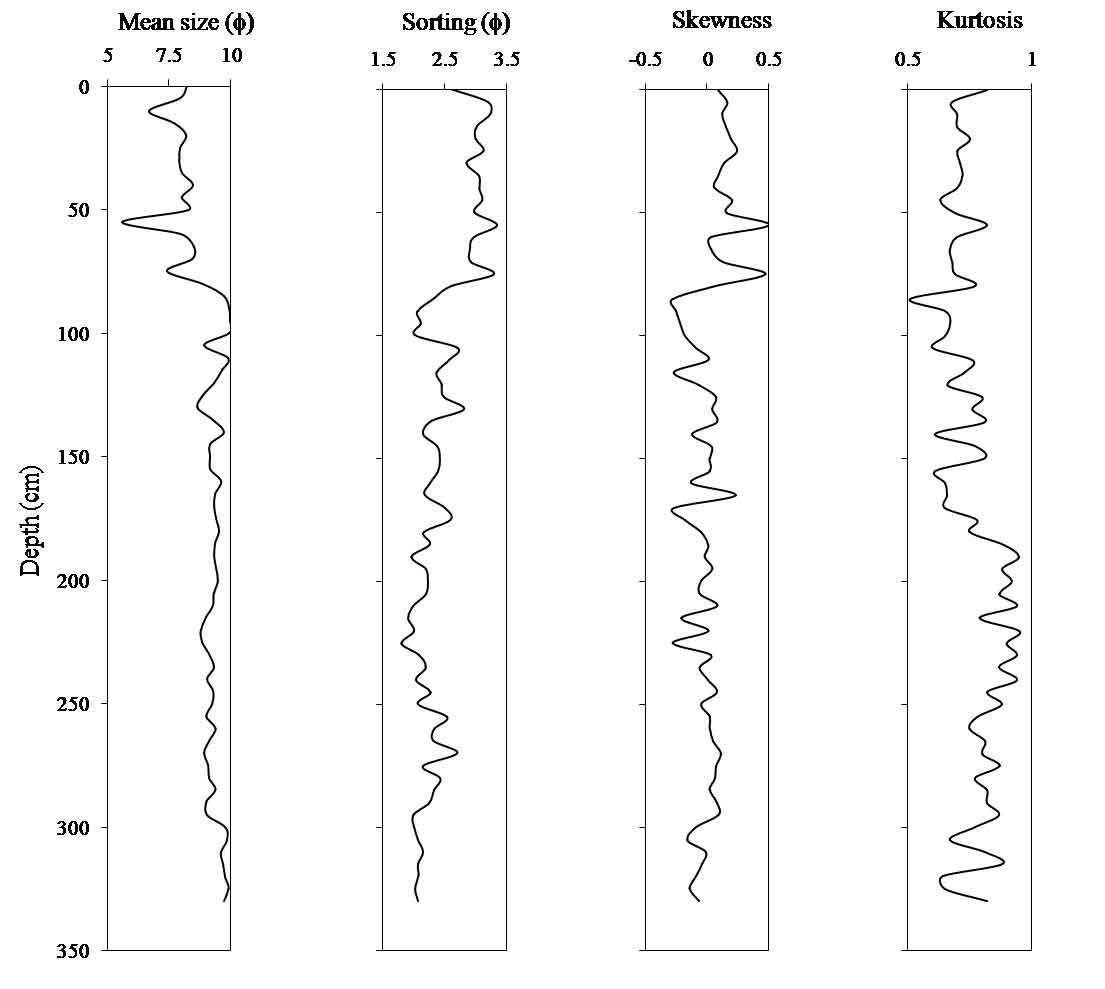
The sediments of the Vaghad Tank characterized by medium silt and clay because the range of mean size is between 5.6 and 9.97f (Table 1). The sorting values fall in the range of 1.8 and 3.35f and imply that the sediments characterized by poorly sorted to very poorly sorted category. The skewness values vary from -0.28 to 0.50. Both the negative (excess coarse material) and positive (excess fine material) skewness values were observed in this pit. The kurtosis values vary between 0.52 and 2.0 and suggest that the grain-size distribution ranges from platykurtic to very leptokurtic (Table 1).

Vertical variation in the statistical parameters of grain-size for the Vaghad Tank has shown in figure 6. It is evident from the plot that considerable variation observed in all the statistical parameters, roughly up to 150 cm from top and then less variation observed within the basal unit (Figure 6). Relatively, negative trend noticed between mean sizes and sorting index, which indicate that as mean size increases there is a decrease in the values of sorting. The uppermost part of the section has characterized by coarse material, while fine material dominates the lower part of the section. The lowest mean size, sorting, skewness and kurtosis values observed at the depths of 55, 225, 225 and 85 cm and highest values occur at 95, 55, 55 and 190 cm depth, respectively (Figure 6).

Figure 6. Vertical variation in the grain-size parameters

4.4 Mineral Magnetic Measurements

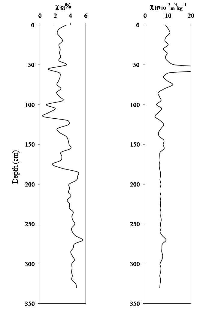
From the mineral magnetic data (Table 2), it is evident that the average of percentage frequency dependent susceptibility of the samples is 3.37% and it varies between 0.45 and 5.59%. The magnetic susceptibility ranges from 4.32 to 37.54*10^-7m³ kg^-1 and the mean is 9.97*10^-7m³ kg^-1.

Inverse trends observed for both the parameters. Whereas the magnetic susceptibility shows an increase towards the top, the values of percentage frequency dependent susceptibility shows a decline. Another important feature of the pit is a sudden increase in the c_lf at a depth of 55 cm from top suggesting more concentration of magnetic minerals (Figure 7). The upper portion of the profile has characterized by more variation while lower portion shows less variation in the magnetic properties.

Figure 7. Results of frequency dependent susceptibility and magnetic susceptibility values

4.5 Relationship between Textural Classes and Magnetic Susceptibility

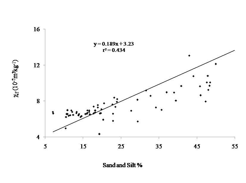
Figure 9 shows the correlation between textural classes (sand and silt %) and magnetic susceptibility. It indicates positive relationship between sand silt (%) and magnetic susceptibility. The magnetic susceptibility increases with the increase in the percentage of sand and silt. The concentration of magnetic minerals observed more in the sand and silt sized particles in the deposits.

The plots shown in the figure 8 indicate negative relationship between percentage of clay and magnetic susceptibility (c_lf). Generally, as percentage of clay increases, there is decrease in the magnetic susceptibility.

Figure 8. Relationship between the percentage of clay and the magnetic susceptibility

Figure 9. Bivariate plot of sand silt and magnetic susceptibility

The low mineral magnetic concentration (average c_lf is 7.97*10^-7m³kg^-1) is noticed in the Vaghad Tank sediments which correspond to the low percentage of silt and sand. The tank sediment constitutes very high percentage of clay.

4.6 Geochemical Analyses

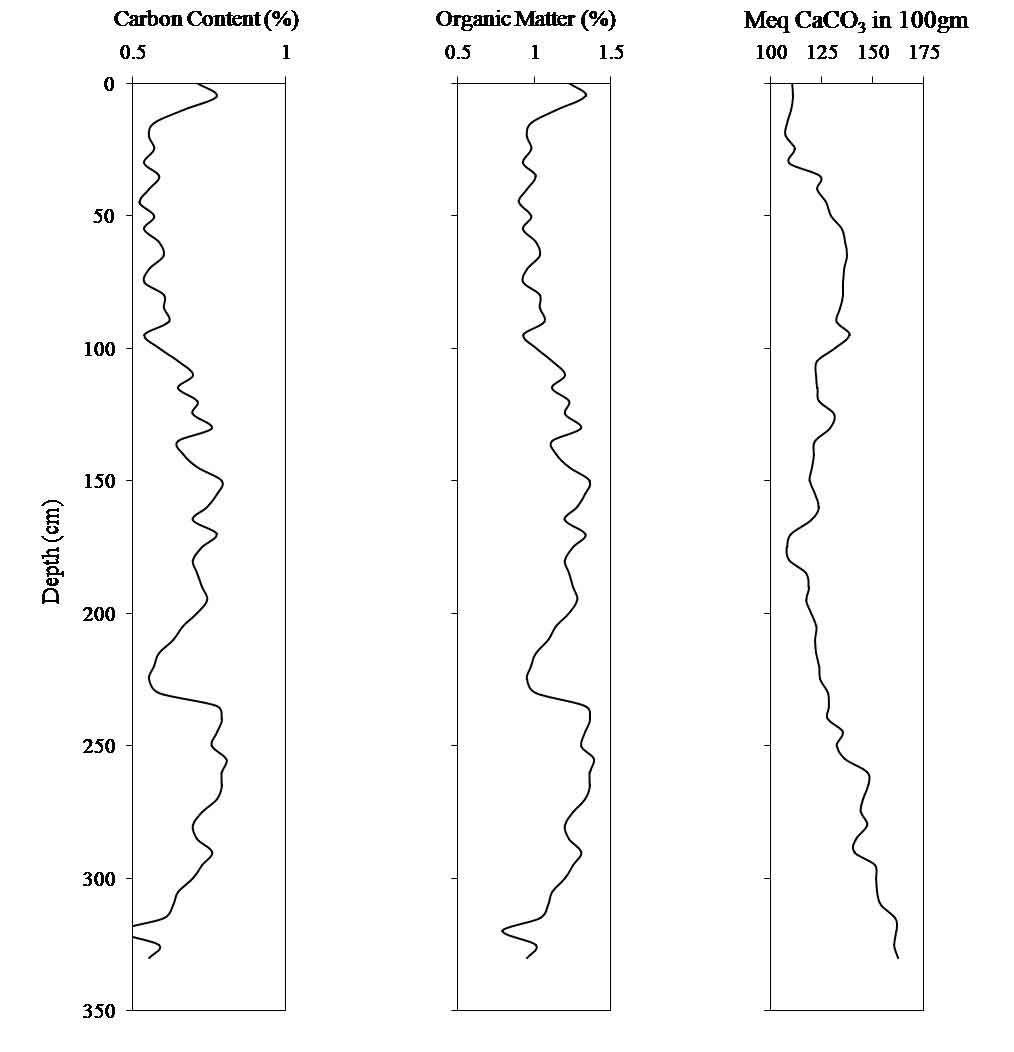
The results of carbon content, organic matter and CaCO₃ in the sediments of the Vaghad Tank presented in table 2. The values of carbon content lay between 0.46 and 0.81% and organic matter ranges from 0.79 and 1.39%. The CaCO3 varies between 107.50 and 162.50. The average amounts of carbon content, organic matter and CaCO₃ are 0.66%, 1.14% and 129.98%, respectively (Table 2).

Figure 10 shows the vertical variation in the geochemical parameters of the Vaghad Tank sediments deposits. The percentage of carbon content and organic matter progressively increases from top to bottom except at the level between ~200 and ~230 cm and bottom part of the profile. The plot of calcium carbonate indicates general increase in the values of CaCO₃ from top to bottom. The lowest amount of CaCO₃ has seen in the uppermost and middle part of the section (Figure 10). The lowermost part of the profile has characterized by lowest organic matter and highest calcium carbonate, possibly due to low rainfall. During low rainfall events, in general, the growth of vegetation is less and more evaporation from the water bodies.

Figure 10. Vertical variation in carbon content, organic matter and calcium carbonate

5 . DISCUSSION

Many palaeoclimatic studies have shown that the multi-proxy data of the tanks sediments provide information about rainfall and runoff conditions prevailed in the catchments of the tanks. Several earlier sedimentological and geochemical studies of sediment deposits of various environments found a good relationship between proxy data (texture, geochemical and mineral magnetic parameters) and hydrodynamic conditions of the catchments (Thompson et al., 1975; Dearing et al., 1981; Oldfield, 1991; Basavaiah and Khadkikar, 2004; Sangode et al., 2007; Shankar et al., 2006; Warrier et al., 2011). A positive relation between low-frequency magnetic susceptibility (χ_lf) and rainfall conditions has found in the studies by Shankar et al., (2006). The study shows that during high rainfall events, the fluxes of the particles of sand and silt is more in the tank and during low rainfall events, the proportion of clay particles is more in the tank sediments. High proportion of sand and silt in the deposits contains more mineral magnetic particles and high proportion of clay constitutes less mineral magnetic particles. Presents study have also established a positive relationship between sand, silt particles and magnetic susceptibility and negative relation between clay and magnetic susceptibility.

A number of past monsoon variability studies based on various proxy and historical records has been carried by many workers such as Abhyankar (1987), Yadava et al. (2004), Kale and Baker (2006), Shanker et al., (2006), Adamson and Nash (2014), etc. Severe fluctuations of rainfall have been identified by Abhyankar (1987) on the basis of historical records from western India. The study suggests that a general increase in the droughts from 16^th century and frequency of droughts increased in the 18^th and 19^th century. In the earlier part of 20^th century, frequency of failure of rainfall was low but increased in later half of the 20^th century (Abhyankar, 1987). A noteworthy increase in the southwest monsoon during the past four centuries inferred based on fossil Globigerina bulloides from Arabian Sea by Anderson et al., (2002).

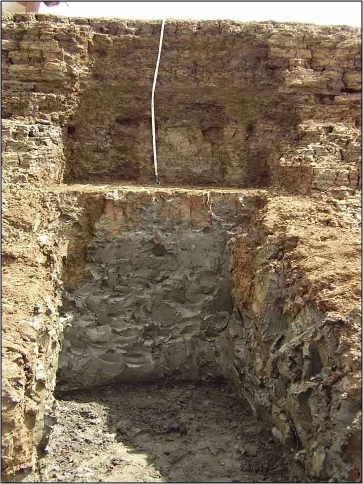
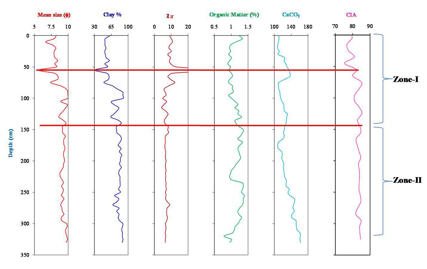
 The results of the present study, demonstrated that the vertical variations in the textural, mineral magnetic and geochemical characteristics of the Vaghad Tank sediments reveal some minor changes in the sediment flux in the upper units of the lithosection (Figure 11). Vaghad Tank, which is located in the sub-humid part, shows that the lower (and older) sediments (below ~150 cm depth) are more or less similar in terms of grain-size, magnetic susceptibility and geochemical parameters. At the depth of ~50 cm from the top, significant variation observed in the sediment characteristics.  The upper (and younger) sediments up to the level of ~150 cm from the top of the lithosection show considerable variations in the sediment characteristics. The sediment section of Vaghad Tank can roughly be divided into two major sections on the basis of properties of sediments i.e. Zone-I (Top to ~150 cm) and Zone-II (~150 cm to bottom) (Figure 11).

Figure 11. Combined plot of vertical variation in multiproxy data

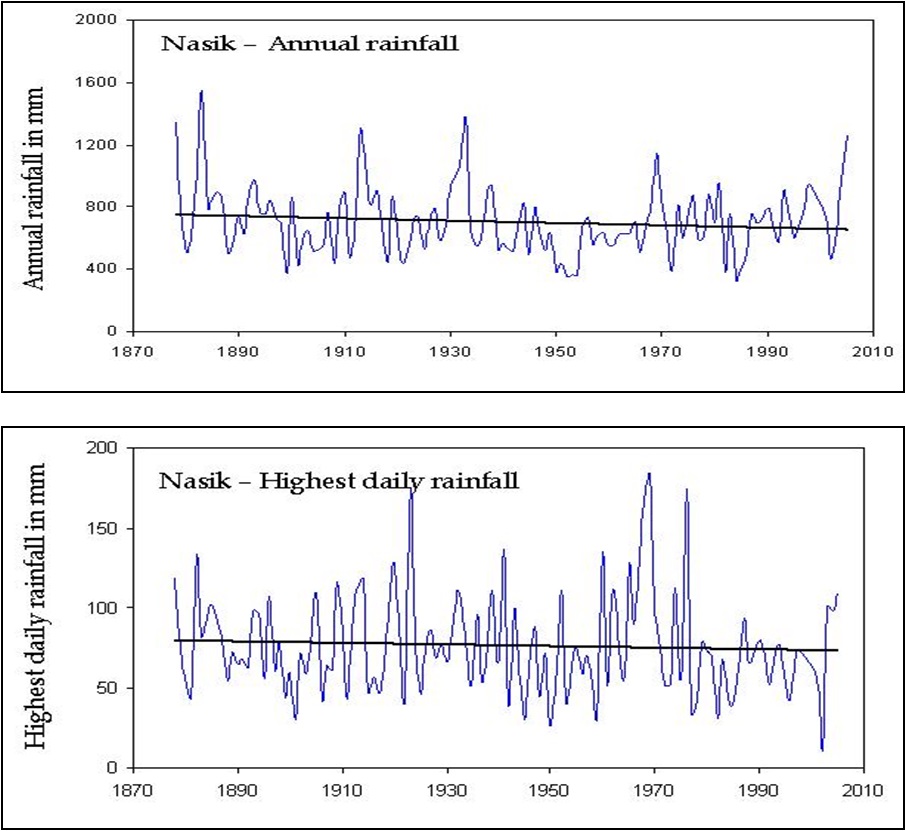
Complete absence of gravelly units and presence of some sandy units in the upper section of the tank deposits indicate that the hydrological conditions have changed slightly in the later stages of sediment deposition. The occasional intense monsoon spells, produce large amount of runoff. The sediments associated with such events are often slightly coarser than those of deposited during low intensity rainfall events, because of high specific energy. Such intense rain-spells are very common in monsoon dominated areas and do not necessarily represent a change in overall climatic conditions. The minor variations in the grain-size in the tank deposits perhaps only represent such high-magnitude random events. Therefore, based on sediment properties of the Vaghad Tank, it appears that the past monsoon rainfall conditions have changed slightly during the last few decades (Zone-I) and the past monsoon rainfall conditions were more or less similar during the early few decades (Zone-II). A very high rainfall event may be attributed to the major variations in the sediment properties at the depth of ~50 cm (Figure 11). The prominent variations in the upper part of the sedimentary records of the Vaghad Tank could be attributed to the changes in the land use or vegetation cover within the Vaghad Tank catchment area as there is no any significant trend in the annual rainfall of Nashik Station in the last century (Figure 12).

Figure 12. Time series plot of annual and highest daily rainfall

The major limitation of the present study is that the dating techniques have not used for analysis of sediment dates. Chronological data of the tank records are essential to establish the exact timing of the changes identified in the sedimentary sequences, as well as to estimate the sedimentation rates.

6 . CONCLUSIONS

The textural, mineral magnetic and geochemical characteristics of the Vaghad Tank deposits have provided information about the past monsoon variability prevailed in the catchment area of the tank.  The results of the study shows some minor variations in the properties of sediments up to ~150 cm from the top of the lithosection and this can be attributed to the minor changes in the past monsoon conditions and/or changes in the landuse pattern. The results also reveal a sedimentary unit at the depth of ~50 cm with major difference in the multi-proxy data and this can be attributed occasional intense monsoon spells in the catchment area. Overall, sedimentary profile does not exhibit any systematic trend in the sediment properties. Finally, based on results of the present study, we conclude that no significant changes in the past monsoon conditions have been occurred during the last century but some minor changes in the hydrodynamic conditions have been noticed during the last few decades.

Tables

Figures

Conflict of Interest

Acknowledgements

Abbreviations

References

1.
Abhyankar, H. G., 1987. Late Quaternary palaeoclimatic studies of western India. Unpublished PhD Thesis, submitted to the University of Poona, Pune.
Basavaiah, N. and Khadkikar, A. S., 2004. Environmental magnetism and its application towards palaeomonsoon reconstruction. Journal of Indian Geophysical Union, 8, 1-14.
Brown, A. G., 2003. Global environmental change and the palaeohydrology of Western Europe: A Review. In: Palaeohydrology, Understanding Global Change, K.J Gregory and G. Benito (eds.). John Wiley and Sons Ltd, Chichester, 105-121.
Chauhan, M. S., Mazari, R. K. and Rajagopalan, G., 2000. Vegetation and climate in upper Spiti region, Himachal Pradesh during late Holocene. Current Science, 79, 373-377.
11.
Collinson, J. D. and Thompson, D. B., 1989. Sedimentary structures. Unwin Hyman Ltd, London, 2.
Gupta, A.K. and Thamban, M., 2008. Holocene Indian monsoon variability. Glimpses of Geoscience Research in India, The Indian Report to IUGS 2004-2008, edited by Singhvi, A.K., Bhattacharya, A. and Guha, S., INSA, New Delhi, 28-31.
Kale, V. S., Gupta, A., and Singhvi, A. K., 2003. Late Pleistocene-Holocene Palaeo-hydrology of monsoon Asia. In: Palaeohydrology, Understanding Global Change. K.J Gregory and G. Benito (Eds.). John Wiley and Sons Ltd, Chichester, 213-232.
Pant, R. K., Phadtare, N. R., Chamyal, L.S. and Juyal, N., 2005a. Quaternary deposits in Ladakh and Karokoram Himalaya: A treasure trove of the palaeoclimate records. Current Science, 88, 1789-1798.
35.
Pawar, N. J., Kale, V. S., Atkinson, T. C. and Rowe, R. J., 1988. Early Holocene waterfall tufa from semi-arid Maharashtra plateau (India). Journal Geological Society of India, 32, 513-515.
36.
Pettijohn, F. J., 1975. Sedimentary Rocks. Harper and Row Publishers, New York, 24-26.
Sangode, S. J., Sinha, R., Phartiyal, B., Chauhan, O. S., Mazari, R. K., Bagati, T. N., Suresh, N., Mishra, S., Kumar, R. and Bhattacharjee, P., 2007. Environmental magnetic studies on some quaternary sediments of varied depositional settings in the Indian sub-continent. Quaternary International, 159, 1-134.
41.
Sant, D. A., Krishna, K., Rangarajan, G., Basavaiah, N., Pandya, C., Sharma, M. and Trivedi, Y., 2004. Characterization of flood plain and climate change using multiproxy records from Mahi River Basin, Mainland Gujrat. Journal of Indian Geophysical Union. 8, 39-48.
42.
Shankar, R., Prabhu, C. N., Warrier, A. K., Vijaya Kumar, G. T. and Sekar, B., 2006. A multi-decadal rock magnetic record of monsoonal variations during the past 3,700 years from a tropical Indian tank. Journal Geological Society of India, 68, 447-459.
Sinha, R., Stueben, D. and Berner, Z., 2004. Palaeohydrology of the Sambhar Playa, Thar Desert, India. Journal Geological Society of India, 64, 419-430.