1 . INTRODUCTION
Groundwater is one of the most natural resources that support human health and ecological diversity, but nowadays it is decreasing and there is an increase in demand for water (Lakshmi and Reddy, 2018). It’s also known as the water that occupies all of the pore space in soils and geologic formations beneath the water table (Wudad et al., 2021). It flows through the aquifer layer towards the discharge point such as wells, springs, rivers, lakes and the oceans (Bekele, 2021). Groundwater is also recognized as one of the most valuable natural resources, an immensely important and dependable source of water supply in all climatic regions all over the world (Debele, 2020).
Ethiopia is one of the countries in Africa known for abundant water resources but minimum utilization of groundwater for irrigation, domestic purposes and livelihood (Berhanu and Hatiye, 2020). The main part of Ethiopian areas has a shortage of rainfall and water scarcity due to a fluctuation in climate (Andualem and Demeke, 2019). The population of Didessa Sub-basins has used waters for drinking and other livestock from ponds and others by going long travel to fetch the water from rivers. The decreased rainfall in the arid zone and increasing population size and demands of water for irrigation and other livelihood requirements urges sustainable exploitation of the groundwater resources in the region (Kindie et al., 2019; Mengistu et al., 2019). In the study area, there is a large demand for groundwater development and utilization. However, there is a lack of in-depth understanding of the groundwater potentials in Ethiopia. In the recent past, the best estimates of the country’s exploitable groundwater potential ranged between 12 and 30 billion cubic meters (Berhanu, 2014). The groundwater potential inside Ethiopia’s territory was estimated to be around 1000 billion cubic meters based on hydrogeological parameters (Kebede, 2013). Other studies have found a different amount for Ethiopia’s groundwater potential about 40 billion cubic meters (Mengistu et al., 2019; Berhanu and Hatiye, 2020). Furthermore, there were just a few studies on the groundwater potentials of smaller catchments. As a result, there is a compelling need to investigate and develop the nation’s groundwater resources so that more people, particularly in rural areas, can benefit from improved water supplies. On the other hand, there is very little research in Ethiopia on the use of groundwater for irrigation (Mengistu et al., 2021). This could be due to a lack of knowledge about the existing groundwater resource and the necessity for big upfront investment in groundwater development for irrigation in the country (Berhanu and Hatiye, 2020). Groundwater potential investigation may thus be a necessary step in ensuring the nation’s long-term usage of groundwater for a variety of needs, including household, agricultural, and industrial uses (Mengistu et al., 2021; Dile et al., 2018). However, extensive use of groundwater based on only limited information may cause unsustainable use of the resource. Subsurface studies are often carried out when there arises a need for local specific development of groundwater exists including borehole, spring, shallow or hand-dug wells for domestic water supply (Wudad et al., 2021). Unsustainable groundwater use is becoming a visible problem and a major source of concern for many developing countries (Hussein et al. 2016). One of these problems is the absence of updated spatial information on the quantity and distribution of groundwater resources (Mengistu et al., 2021). Nowadays, there is a strong need to use groundwater for socio-economic development in Ethiopia, especially in rural areas (Dile et al., 2018). The ministry of water resources, through the water well design and monitoring enterprise, has performed a multi-disciplinary study incorporating hydrogeology and geophysics to investigate Ethiopia’s groundwater potential by employing time-consuming and costly geophysical and hydrogeological procedures, the potential can be realized. Aside from that, the groundwater potential for the Didesa sub-basin has not been characterized in prior research using GIS and RS approaches, separately (Kindie et al., 2019; Mengistu et al., 2019; Bashe, 2017). Since there is a limitation of previously work done in the area of the potentials and recharge zone in detail, the present study fills the gap by applying GIS and remote sensing techniques. These techniques are very easy to access, identify groundwater potential, and recharge zone of large and inaccessible areas (Gidey, 2018; Wudad et al., 2021; Mengistu et al., 2021; Andualem and Demeke, 2019). Considering the problems and the gaps from the other studies in terms of cost and time, an increasing number of population densities and fluctuation of climate on water scarcity in Didessa Sub-basins, this research focused on identifying the potential and mapping the spatial and temporal distribution of groundwater availability in the study area.
The availability, accessibility, movement, and occurrence of groundwater depends on geology, slope aspect, lineaments, drainage density, LULC, Rainfall, surface runoff, and geomorphology of the area (Wudad et al., 2021; Kindie et al., 2019; Bekele, 2021; Debele, 2020). Evaluation, exploitation, exploration, site selection/delineation, and maps of groundwater need serious caution as it is cost and time-effective (Tamiru and Wagari, 2021; Ahmad et al., 2020). It is out of our site improper evaluation of groundwater and site selection is mostly expected to pose the problem.
There are several methods available for the investigation of groundwater exploration or its availability in the sub-surface environment. They range from the oldest traditional water dowsing methods to the recent electromagnetic resonance (EMR) technologies (Wudad et al., 2021). In general, all the methods can be categorized into two broad classes: surface and sub-surface. The most cost-effective and simple methods of groundwater exploration or potential assessment are those that take place on the surface (Gintamo, 2014). Surface geophysical approaches, as well as esoteric geomorphological, geological, soil related, and microbiological remote sensing techniques, are among these technologies. The sub-surface methods mainly consist of test drilling of boreholes and geophysical logging techniques (Bashe, 2017; Tamiru and Wagari, 2021). Although the sub-surface methods are accurate for groundwater exploration, they incur large investment since drilling, completing and development of wells may be needed for the effective application of these methods (Bawoke et al., 2020; Melese and Belay, 2021). Therefore, it is a usual practice to undertake surface investigation methods for locating potential groundwater sources (Gidey, 2018). Remote sensing technique integrated with GIS is becoming a potent tool for the identification and mapping of groundwater potential zones in a time and cost-effective manner (Berhanu and Hatiye, 2020; Kindie et al., 2019; Bekele, 2021). GIS and remote sensing approaches are particularly effective in the identification of groundwater potential of any region and often use spatial data to analyze and characterize required information (Abiy et al., 2014). The geographic information system uses some proxy data from the ground surface to examine subsurface phenomena or objects. Geology, often known as lithology, is the study of rocks and minerals. landforms or geomorphology groundwater potential zones are typically identified using drainage density, rainfall, geological features or lineaments, slope, LULC, and soil properties (Melese and Belay, 2021; Debele, 2020; Kahsay et al., 2019). These data were used as proxy data for groundwater potential mapping in this study. When there are few direct measurements of groundwater, especially in smaller catchments, using such data to assess groundwater potential for Ethiopian conditions is extremely beneficial (Tamiru and Wagari, 2021; Kindie et al., 2019; Mengistu et al., 2021). The Didessa sub-basin is not exceptional to this constraint and there have been no previous investigations on the sub-basin’s groundwater potential. The goal of this work was to use GIS and remote sensing approaches to identify and map the groundwater potential zones in the Didessa sub-basin using groundwater proxy data. The study also aimed to test the veracity of the qualitative analysis GIS and remote sensing techniques yielded. Groundwater potential maps that have been found and organized may provide information on productive wells in the research area. The findings could be utilized as a geo-database to help decision-makers and other stakeholders in the research area appropriately use and manage groundwater resources.
Geographical Information System (GIS) and Remote Sensing (RS) are the optional methods to provide all parameters which influence the groundwater potential of one area and it can access, manipulate, and analyze the spatial and temporal data from satellite images (Yifru et al., 2020; Adeyeye et al., 2019). Besides this, Gupta and Srivastava (2010) explain many decision-making analysis approaches such as Multi-Criteria Decision-Making (MCDM), Analytical Hierarchy Process (AHP) (Wind and Saaty, 1980), and Fuzzy Logic to fill the gap of water scarcity and decision-making on groundwater potential zone for evaluation and mapping. AHP is useful method for complex decision-making. A pairwise comparison matrix is used for checking the consistency ratio (Dinka et al., 2014; Wind and Saaty, 1980). These decision-makers use this to reduce the bias in decision-making (Wind and Saaty, 1980; Kahsay et al., 2019). Therefore, this study was focused on the evaluation of groundwater potential zone in the Didesssa sub-basin by the integrated approach of remote sensing and GIS techniques using the AHP modeling approach. Besides this, the specific objectives of the study were to prepare the thematic maps of the study area such as lithology, LULC, slope, lineaments, soil texture, drainage density, and geomorphology and runoff depth to identify the factors that more affects the groundwater potential and recharge zone to assess, evaluate and delineate groundwater potentials of the area by using remote sensing and geospatial data.
2 . MATERIALS AND METHODS
2.1 Study Area
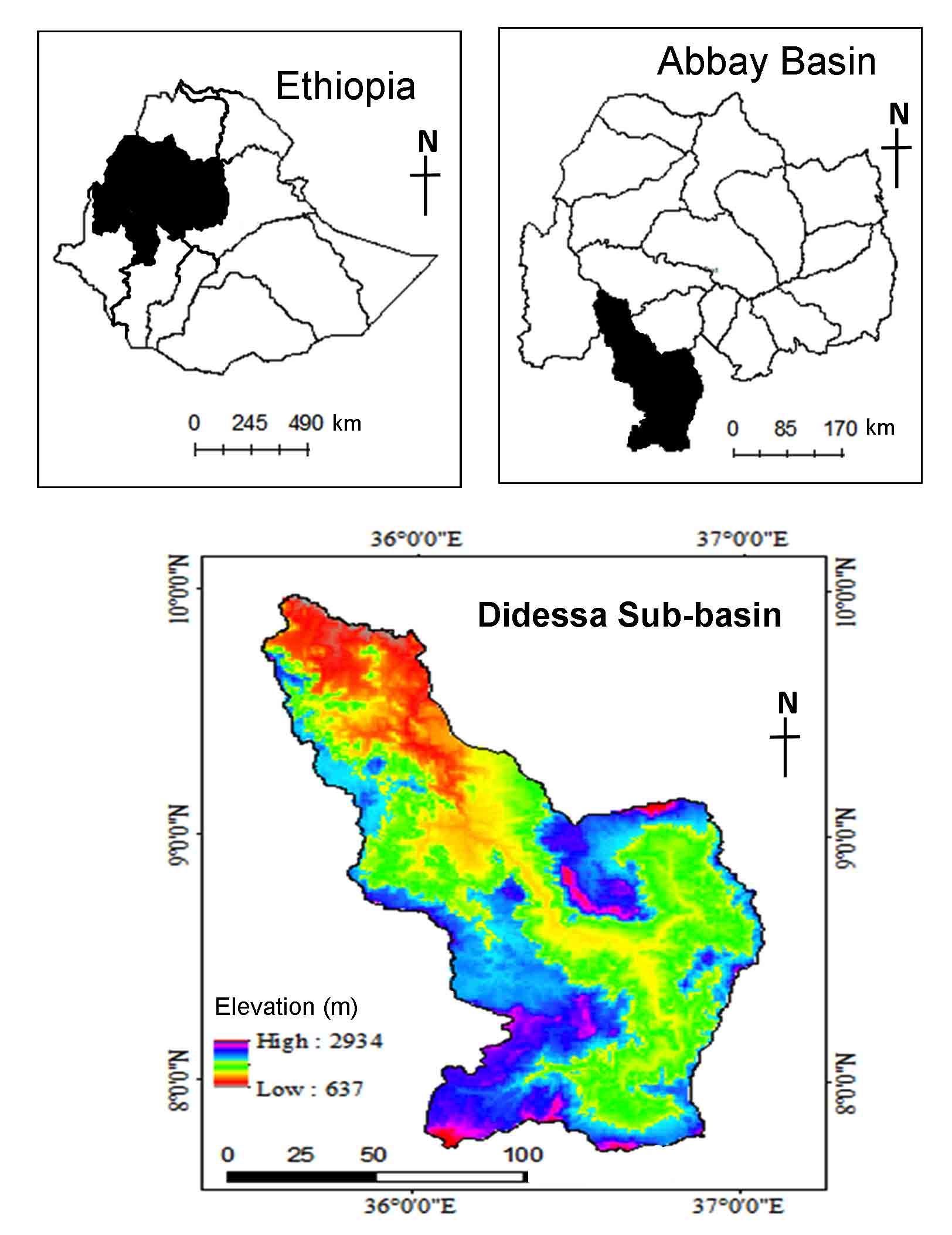
The Didessa sub-basin is the largest among the major sub-basins in Abay Basin in terms of its annual discharge (Kabite and Gessesse, 2018). In the Blue Nile basin, the Didesa sub-basin is the most important both hydrologically and physiographically. The Nile basin, which has supported millions of people since prehistoric times, receives around 60% of its yearly discharge from the blue Nile river, with the Didessa river accounting about 25% of that discharge (Kabite and Gessesse, 2018). The Didesa sub-basin is located in western Ethiopia, and it encompasses the East and West Wollega zones, the Illubabor zone, the Jimma special zone of the Oromiya area, and some parts of the Kamashi zone of Benishangul Gumuz. Geographically the sub-basin is located between 7º and 9ºN and 35º and 36ºE in the western part of Ethiopia. The elevation in the basin ranges between 654m MSL and 3154m MSL. The river drains an area of 28092km2, and the Didessa River, which is the blue Nile’s greatest tributary, contributes nearly a quarter of the river’s total flow. In the research region, the average annual rainfall is around 1745mm. The river basin is classified under a humid tropical climate with heavy rainfall with an annual amount that is mainly received when the weather is wet. The highest and lowest temperature ranges between 21 and 31ºC and 10 and 15ºC, respectively. Geologically, Didessa sub-basin is dominated by Jimma Volcanic and the central part with Wellega Basalt and the lower parts are dominated by undifferentiated lower complex, Wellega Basalt and Adigrat Sand Stone.
2.2 Data
In this study, eight thematic layers (drainage density, rainfall, slope steepness, LULC, lineaments density, soil, geomorphology, and lithology) were used. The rainfall map was prepared using Inverse Distance Weighting (IDW) interpolation of long term mean annual rainfall data recorded at 23 stations. The information of lithology and soil are collected from the Ethiopian Geological Survey. These thematic layers were prepared with the help of ArcGIS 10.7 platform. The drainage and lineament density maps have been prepared using the line density analysis tool in Arc GIS 10.7. The slope and drainage density were derived from the Shuttle Radar Terrain Mapping Digital Elevation Model (STRM DEM) of 30m resolution. Landsat-8 Operational Land Imager (OLI) satellite images were obtained from the United States Geological Society (USGS) website and used to generate the lineament density and LULC maps.
Table 1. Data
|
Data
|
Sources
|
Remarks
|
|
Annual rainfall (1998-2016)
|
National Meteorological Agency (NMA)
|
Areal rainfall map prepared using IDW technique.
|
|
SRTM DEM 30m
|
https://earthexplorer.usgs.gov/
|
Used to prepare the elevation, drainage density and slope maps
|
|
Landsat-8 OLI/TIRS
|
https://landsatlook.usgs.gov/
|
Used for mapping of lineaments, LULC and geomorphology.
|
|
Maps
|
Ethiopian Geologic Survey
|
Procured lithological and soil maps
|
2.3 Methodology
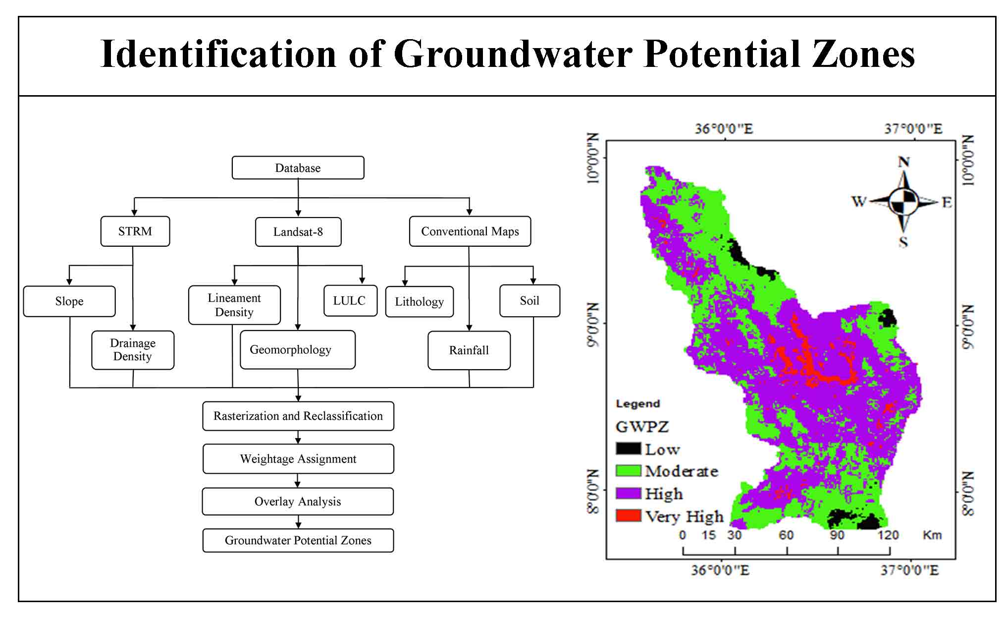
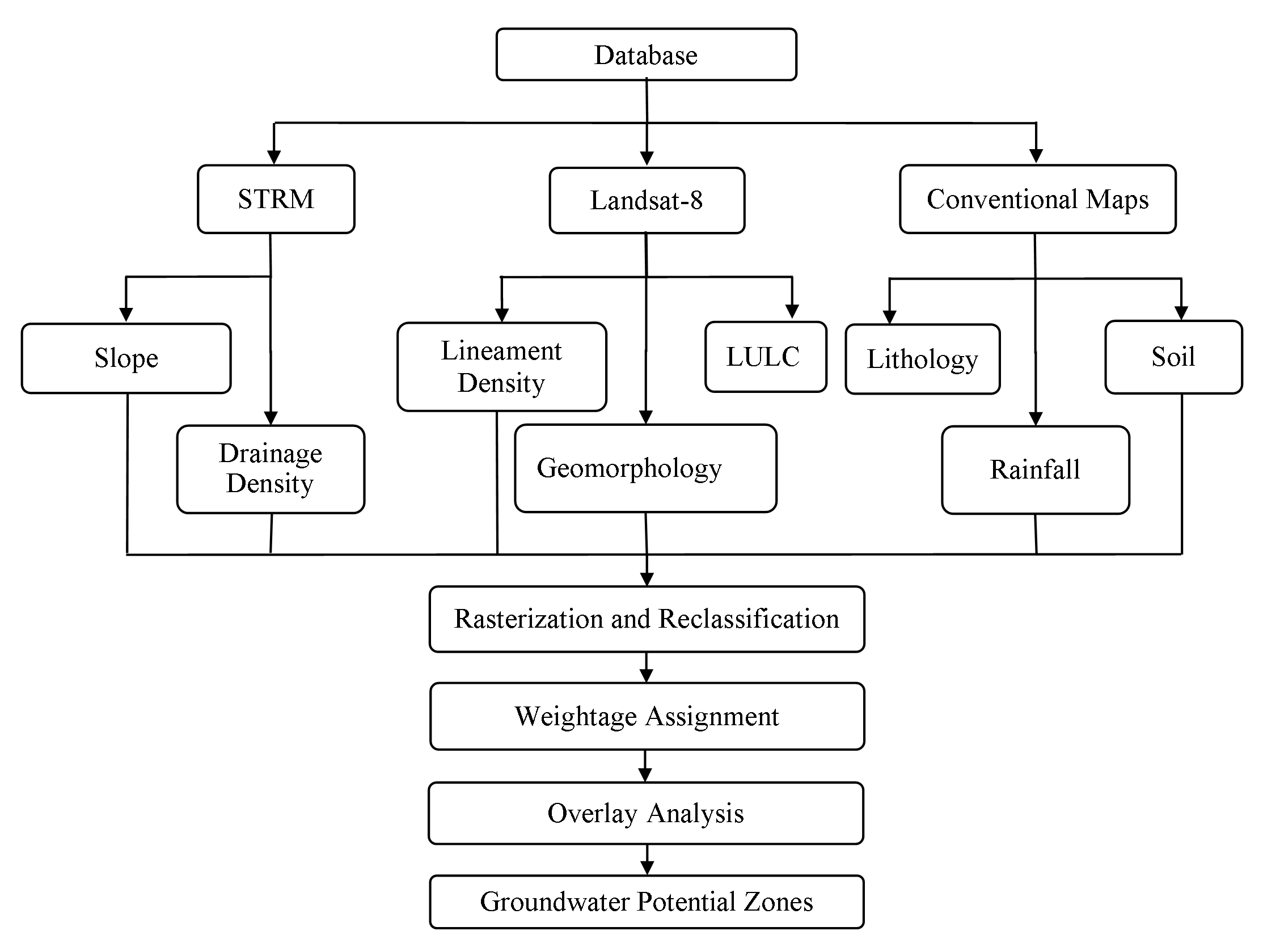
GIS and remote sensing techniques were applied to delineate the groundwater potential of the Didesa sub-basins through the AHP. The methodology used in this work includes the stages: i) identification and evaluation of criteria, ii) data collection, iii) preprocessing, iv) input dataset, vi) reclassified input layers, vii) pairwise comparison of criteria and give weight with AHP, and x) overlay analysis with weight sum overlay analysis in ArcGIS tools and ranking the final value (Figure 2). The long-term average point rainfall values were used to generate areal rainfall map. IDW interpolation approach was used to interpolate the areal rainfall map. Twenty-three stations data were employed for the preparation of areal rainfall of the study area. In this study, data sets such as SRTM data, Landsat-8, and geological data of the study area is identified and used as input data sets for further processing. SRTM at 30 X 30m resolution was used to generate digital elevation model of the area. Landsat images have been used for the preparation of LULC, lineament density and geomorphology maps. Then the elevation map of the Didessa sub-basin was prepared using Arc GIS. Further, the elevation data was used to generate the slope raster data in each grid cell. In the elevation raster, slope was measured by the identification of maximum rate of change in value from each cell to neighboring cells. The slope classes in the watershed were identified using slope spatial analyst tool in the ArcGIS package. On the other hand, the data related to drainage density were generated indirectly from the watershed slope data. Drainage density is defined as the closeness of spacing of stream channels. Drainage density (Dd) is the measure of the total length of the stream segment of all orders per unit area. The lineaments of the study area were extracted from the Landsat-8 OLI/TIRS image (path 170, row 51 with zero cloud cover) using automated processing LINE tool in PCI Geomatica 2017. Out of the 11 bands of the Landsat-8 OLI/TIRS images, the lineaments were extracted from band 5 due to its quality and the highest number of lineaments delineated. After the lineaments were extracted, further processes of editing the watershed divide line and road features were done in GIS to ensure the quality of the extracted lineaments. The geomorphological map of the study area was prepared following the Hammond landform classification technique.
2.3.1 Weight Assessment and Normalization
Because of all parameters do not have an equal effect on groundwater distribution a ranking of each parameter is needed. Weighting each factor and a pairwise comparison matrix were prepared for each map based on Wind and Saaty (1980) scale. The score for the classes in a layer and weights for each factor was assigned and a pairwise comparison matrix has been prepared for each map by using the Multi-Criteria Decision Analysis technique based on AHP (Wind and Saaty, 1980) by considering seven factors (lithology, lineament density, soil, and drainage, rainfall, slope and LULC). On Saaty’s scale of 1 to 9, each criterion is compared to the other criteria, proportionate to its relevance in matrices (Table 2). The score for classes in a layer and weights for thematic layers of each factor were calculated using the pairwise comparison matrix was carried out by using AHP techniques (Moges et al., 2019). The relative weight of their relevant classes was taken into account while calculating the cumulative weight of the primary criteria. Map categorization and weight assignment for groundwater potential and recharge parameters selected for groundwater potential and nine parameters selected for groundwater recharge potential zone. Normalization of assigned weight using AHP (Wind and Saaty, 1980) based on Saaty’s scale were considered two themes and classes at a time based on their relative importance to determine the groundwater potentials and recharge zone. Following that, pairwise comparison matrices with given weights to various thematic layers and classes created with the help of AHP and weights normalized by the eigenvector approach. To assess the normalized weights of various thematic layers and their particular classes, the consistency ratio (CR) was determined according to Wind and Saaty, (1980). To compute the CR of various thematic layers and their classes, the following steps were carried out:
1. Square matrix: A = aij (Equation 1) the element of row i column j was produced and the lower triangular matrix was completed by taking the reciprocal values of the upper diagonal using the formula, aij = 1/aij
\(A = \begin{bmatrix}\frac{P1}{P1} & \frac{P1}{Pj} & \frac{P1}{Pm}\\[0.3em] \frac{Pi}{P1} & 1 & \frac{Pi}{Pm} \\[0.3em]\frac{Pn}{P1}& \frac{Pn}{Pj} & \frac{Pn}{Pn} \end{bmatrix}\) (1)
2. Summation of all columns j in the matrix from (Equation 1) using (Equation 2)
\(\frac{P1}{P1} \ldots \ \ldots+ \frac{Pi}{Pj} \ldots \ \ldots \ \ldots \frac{Pn}{Pn} = \frac{\sum_{i=1}^{n} Pi}{Pi}\) (2)
3. Divide each element of matrix aij = pi/pj (Equation 2) by (Equation 3) to get normalized relative weight (Equation 5)
\(\frac{\frac{Pi}{Pj}} {\frac{\sum_{i=1}^{n} Pi}{Pj}}= \frac{Pi}{Pj} \times \frac{Pj}{\sum_{i=1}^{n} Pi} = \frac{Pi}{\sum_{i=1}^{n} Pi} \) (3)
4. Averaging across the rows (Equation 6) to get the normalized Principal Eigenvector (priority vector) i.e., Rate (Ri) or weight of row ‘i’ (Wi). Since it is normalized, the sum of all elements in the priority vector should be one.
\(\frac{Wi}{Ri}= \frac {Pi} {\sum_{i=1}^{n} Pi} \ldots \ \ldots+ \ \ldots\frac {Pi} {\sum_{i=1}^{n} P1} \times 1/n \) (4)
The judgments of the pairwise comparison within each thematic layer were checked by the consistency ratio (Wind and Saaty, 1980). The proportion of consistency scholars recommended that for matrices having a CR rating greater than 0.1, the method should be repeated until the desired value of CR = 0.1 is obtained. The value of CR is computed as (Equation 5)
\(RC = \frac{Ci}{R}\) (5)
where, RI is Saaty’s ratio index; CI is consistency index. Consistency index is a measure of consistency or degree of consistency of the judgment and computed using (Equation 6).
\(CI = \frac{(\lambda max-mn)}{n-1}\) (6)
where, n is the number criterion, the value of RI for n criteria as indicated in Table 2.
To compute \(\lambda max\) , first multiply the normalized value by the respective weight (Equation 6) and then, the values of the product are added together to get \(\lambda max\) (Equation 7)
\(\lambda max = \sum_{i=1}^{n} Wi \times \left (\frac {Pi} {\sum_{i=1}^{n} Pi} \right)\) (7)
where, \(\lambda max\) is the largest Eigenvalue of the pairwise comparison matrix. \(Pi\) is the priority of the alternative and \(Wi\) is the assigned rate/weight.
2.3.2 Overlay Analysis
The final map (Figure 11) was obtained by overlaying all thematic maps using weighted overlay methods after assigning rates for classes in a layer and weights for thematic layers (Kindie et al., 2019; Abiy, et al., 2014; Tamiru and Wagari, 2021), using the spatial analysis tool in are G.I.S 10.7 as shown (Equation 8)
\(GWP= \sum_{i=1}^{n} Wi \times Ri\) (8)
where, GWP is groundwater potential zone; \(Wi\) is the weight for each thematic layer and \(Ri\) ; rates for the classes within a thematic layer derived from AHP.
Table 2. Saaty’s scale of relative importance (Wind and Saaty, 1980)
|
Relative importance
|
Definition
|
|
1
|
Equal importance
|
|
2
|
Weak or slight
|
|
3
|
Moderate importance
|
|
4
|
Moderate plus
|
|
5
|
Strong importance
|
|
6
|
Strong plus
|
|
7
|
Very strong
|
|
8
|
Very very strong
|
|
9
|
Extremely importance
|
Table 3. Pairwise comparison matrix
|
Parameters
|
Rf
|
GM
|
Ld
|
Dd
|
Sl
|
St
|
LULC
|
Lith
|
|
Rf
|
1
|
2
|
3
|
5
|
6
|
4
|
6
|
7
|
|
GM
|
0.5
|
1
|
2
|
3
|
5
|
5
|
6
|
7
|
|
Ld
|
0.333
|
0.5
|
1
|
0.5
|
2
|
4
|
2
|
3
|
|
Dd
|
0.2
|
0.333
|
2
|
1
|
2
|
2
|
2
|
3
|
|
Sl
|
0.167
|
0.2
|
0.5
|
0.5
|
1
|
2
|
3
|
4
|
|
St
|
0.25
|
0.2
|
0.25
|
0.5
|
0.5
|
1
|
3
|
4
|
|
LULC
|
0.167
|
0.167
|
0.5
|
0.5
|
0.333
|
0.333
|
1
|
4
|
|
Lith
|
0.143
|
0.143
|
0.333
|
0.333
|
0.25
|
0.25
|
0.25
|
1
|
|
Total
|
2.76
|
4.543
|
9.583
|
11.333
|
17.083
|
18.583
|
23.25
|
33
|
Table 4. Scores and weightages
|
Theme
|
Dominant effect
|
Suitability
|
Scores
|
Weightages
|
|
Rainfall (mm/year)
|
1967.75 - 2120.67
|
Very High
|
5
|
0.327
|
|
1871.88 - 1967.74
|
High
|
4
|
|
1791.99 - 1871.87
|
Moderate
|
3
|
|
1691.56 - 1791.98
|
Low
|
2
|
|
1538.62 - 1691.98
|
Very Low
|
1
|
|
Geomorphology
|
Low Plateaus
|
Very High
|
5
|
0.242
|
|
Low Plains
|
High
|
4
|
|
Mid Plateaus
|
Moderate
|
3
|
|
Mid Plains
|
Low
|
2
|
|
Low Mountains
|
Very Low
|
1
|
|
Lineament Density (Km/Km2)
|
0.176 - 0.274
|
Very High
|
5
|
0.112
|
|
0.13 - 0.176
|
High
|
4
|
|
0.084 - 0.13
|
Moderate
|
3
|
|
0.032 - 0.084
|
Low
|
2
|
|
0 - 0.032
|
Very Low
|
1
|
|
Drainage Density (Km/Km2)
|
0 - 028
|
Very High
|
5
|
0.106
|
|
0.028 - 0.079
|
High
|
4
|
|
0.079 - 0.123
|
Moderate
|
3
|
|
0.123 - 0.17
|
Low
|
2
|
|
0.17 - 0.27
|
Very Low
|
1
|
|
Slope (degree)
|
0.0 - 2.02
|
Very High
|
5
|
0.0757
|
|
2.02 - 3.89
|
High
|
4
|
|
3.89 - 6.3
|
Moderate
|
3
|
|
6.3 - 9.82
|
Low
|
2
|
|
9.82 - 19.11
|
Very Low
|
1
|
|
Soil Texture
|
Loamy Sand
|
Very High
|
5
|
|
|
Sandy Loam
|
High
|
4
|
0.064
|
|
Loam
|
Moderate
|
3
|
|
Clay
|
Low
|
2
|
|
Heavy Clay
|
Very Low
|
1
|
|
LULC
|
Forest
|
Very High
|
5
|
0.046
|
|
Grassland
|
High
|
4
|
|
Woodland
|
Moderate
|
3
|
|
Agricultural land
|
Low
|
2
|
|
Bare land
|
Very Low
|
1
|
|
Lithology
|
Taramber
|
Very High
|
5
|
0.026
|
|
Basalt
|
High
|
4
|
|
Fluvium
|
Moderate
|
3
|
|
Colluvium
|
Low
|
2
|
|
Marshsoils
|
Very Low
|
1
|
Table 5. Normalized pairwise comparison matrix
|
Parameters
|
R
|
Sl
|
GM
|
Ld
|
Dd
|
St
|
LULC
|
Lith
|
Wt
|
Wt %
|
|
Rf
|
0.3623
|
0.44
|
0.31
|
0.44
|
0.35
|
0.215
|
0.26
|
0.21
|
0.32
|
32.76
|
|
GM
|
0.1812
|
0.22
|
0.21
|
0.26
|
0.29
|
0.269
|
0.26
|
0.21
|
0.24
|
24.22
|
|
Ld
|
0.1207
|
0.11
|
0.1
|
0.04
|
0.12
|
0.215
|
0.09
|
0.09
|
0.11
|
11.2
|
|
Dd
|
0.0725
|
0.073
|
0.21
|
0.09
|
0.12
|
0.108
|
0.09
|
0.09
|
0.11
|
10.65
|
|
Sl
|
0.0605
|
0.044
|
0.05
|
0.04
|
0.06
|
0.108
|
0.13
|
0.12
|
0.08
|
7.57
|
|
St
|
0.0906
|
0.044
|
0.03
|
0.04
|
0.03
|
0.054
|
0.13
|
0.12
|
0.07
|
6.4
|
|
LULC
|
0.0605
|
0.037
|
0.05
|
0.04
|
0.02
|
0.018
|
0.04
|
0.12
|
0.05
|
4.6
|
|
Lith
|
0.0518
|
0.031
|
0.03
|
0.03
|
0.01
|
0.013
|
0.01
|
0.03
|
0.03
|
2.6
|
|
Total
|
1
|
1
|
1
|
1
|
1
|
1
|
1
|
1
|
1
|
100
|
3 . RESULTS AND DISCUSSION
4.1 Rainfall
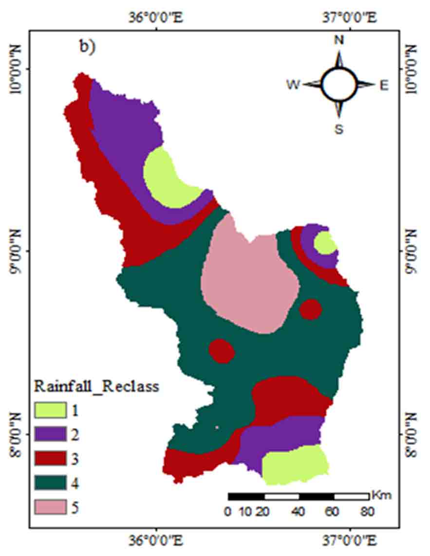
Rainfall is the most important factor for the identification of groundwater potential (Duan et al., 2016). The central and northeastern parts of the study area receive very high rainfall of around 1965-2120mm/year; the most central part receives high rainfall of around 1878-1965mm/year. The northwestern and southern parts receive moderate rainfall 1811-18187mm/year. The Northeastern and few eastern parts of the study area receive low rainfall 1713-1811mm/year. The little eastern southeastern and southern parts receive very low rainfalls (1510-1713mm/year). The high rainfall distribution along high slope gradient in the northwest and southeast highland parts directly affects the infiltration rate groundwater potential zones in the downstream central rift floor of the study area. Based on the mean annual rainfall and its contribution to groundwater potential; the relative weight was given for each rainfall class. The rate was determined by the contribution to groundwater potential; high rainfall areas received a greater weight (Figure 3), while low rainfall areas received the lowest weight indicating low groundwater potential.
4.2 Drainage Density
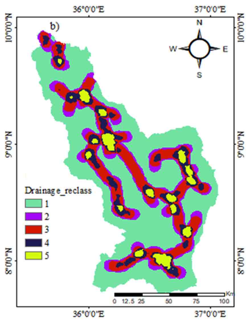
Drainage density is the natural flowing of water runoff to lowland/ common points. It indicates the behavior of surface and subsurface formation, the information of rock, soil permeability, infiltration of water, and surface runoff. Groundwater potential is often weak in places where a higher drainage density is dominant because there is less time for infiltration, whereas areas with a low drainage density allow more infiltration to recharge the groundwater system. Drainage density was prepared from DEM by using line density tool in ArcGIS 10.7 and reclassified into five categories (Figure 4) as very poor = 1 (0-0.02728km/km2), poor = 2 (0.02728-0.07857km/km2), moderate = 3 (0.07857-0.12331km/km2), high = 4 (0.12331–0.170042km/km2), and very high =5 (0.17042–0.2782km/km2). Drainage density is affected by the topographic conditions and the permeability of the geological units. If the slope is flat, the permeability is very high and the drainage density is very low.
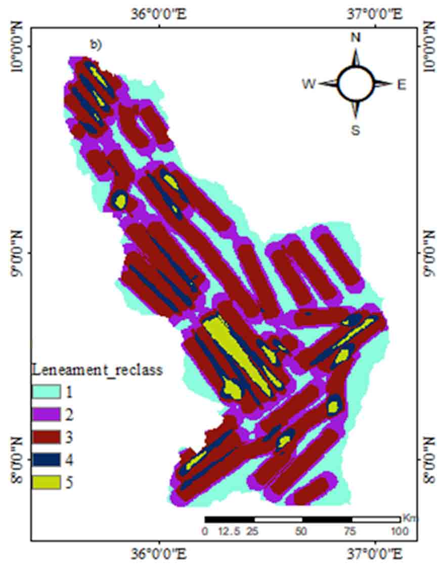
4.3 Lineament Density
Lineaments are the simple and complex linear properties of geological structures. The Geomatica module was used to extract faults, cleavages, fractures, and various surfaces of discontinuities such as terraces and ridges arranged in a straight line or a small curve that are identified by remote sensing lineaments extracted from a single image of Principal Component Analysis (PCA) and record the output as a polyline with vector segment (Tadesse et al., 2015). Due to multispectral imaging bands being often highly correlated, Principal Components used to produce uncorrelated output bands, segregate noise components, and reduce the dimensionality of data sets. This is accomplished by finding a new set of orthogonal axes with their origin at the data mean and which are rotated to maximize the data variance. Landsat images were processed for Principal Component Analysis and eight-bit grayscale lineaments are automatically extracted. Groundwater potential is to be good in areas with a high lineament density. The lineament density was classified into five categories (Figure 5) classified as very poor = 1 (0-0.03234 km/km2), poor = 2 (0.03234-0.08407 km/km2), moderate = 3 (0.08407-0.1304 km/km2), high = 4 (0.1304-0.1767 km/km2) and very high = 5(0.1767-0.2748 km/km2). The large parts of the study areas are classified as moderate lineament density.
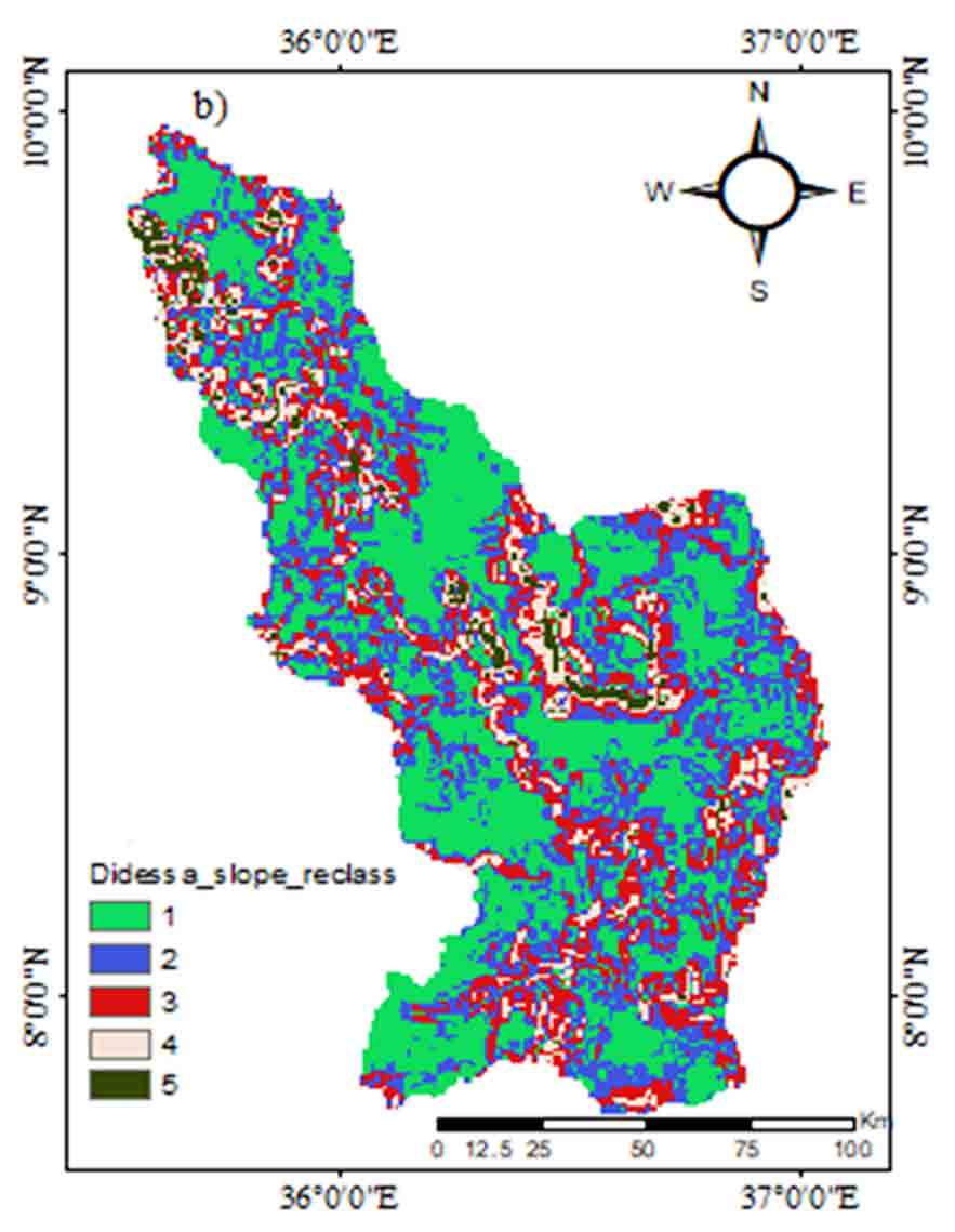
4.4 Slope
The slope is the steepness or the change of elevation between two locations and it has a direct influence on groundwater recharge. High slope regions have high runoff and low infiltration rates that are not suitable for groundwater recharge, because water cannot get enough time to infiltrate to the ground The slope map of the study area was prepared based on the DEM data using the spatial analysis tool in ArcGIS 10.7. Based on this result, the slope of the study area was divided into five classes namely; flat, gentle, moderate, high, and steep slope. The generated map was reclassified (Figure 6) and ranking depend on their groundwater potential and recharge influence. The highest rank was given to flat slope because the flat area can hold water which is very easy for infiltration of water to the ground and the lowest rank was assigned for the steep slope. After all, they result in high runoff and low infiltration which cause low groundwater recharge. For this study, the slopes were reclassified into five categories to groundwater potential zones as very high = 5 (0 - 2.024), High = 4 (2.024 - 3.898), Moderate = 3 (3.898 - 6.297), Poor = 2 (6.297 - 9.82) and very poor = 1 (9.82 - 19.116).
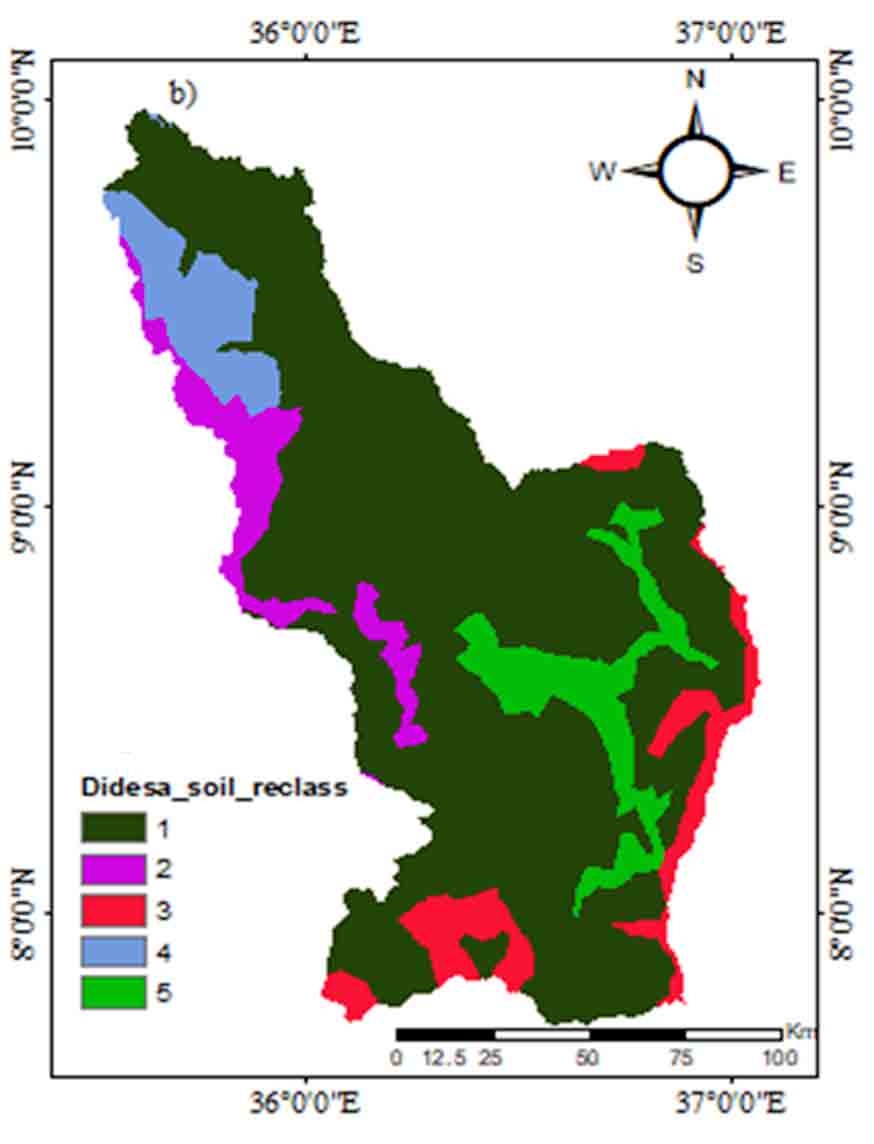
4.5 Soils
Soil is an important factor for delineating the groundwater potential areas. The percolation or infiltration rate of water to the water tables is influenced by soil permeability. Didessa sub-basin is covered by a variety of soil groups. the major soils are Hunitisols which covers (73.77%) and are highly characterized by loam in texture, Hpnitisols (4.66%) with clay texture, Ltleptosols (1.48%) characterized by sandy loam, Hualisols (7.03%), which is loam in texture, Rhnitisols (0.03%) with heavy clay texture character, Dyleptosols (5.73%) which is loamy sand in their texture and Euvertisols (7.3%) characterized by clay texture. The Soils were reclassified into five categories (Figure 7) for groundwater potential zones as very poor = 1 (Heavy clay), poor = 2 (clay), moderate = 3 (loam), high = 4 (sandy loam) and very high = 5 (loamy sand).
4.6 Land Use Land Cover (LULC)
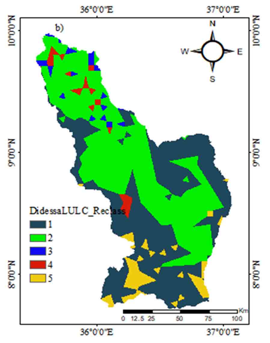
LULC have a direct effect on the hydrological process of surface runoff, evapotranspiration, and groundwater potential. LULC types give the necessary information on infiltration. Water body, agricultural land, and the waterlogged area are excellent sources of groundwater potential, while the bare lands and exposed rock surface areas are less important for groundwater potential. A LULC map was prepared using supervised classification with a maximum likelihood classification from Landsat-8 Operational Land Imager (OLI) Satellite images. Seven dominant LULC namely dominantly cultivated land, shrub land, grassland, dominantly cultivated land, bare land, woodland, and forest are available in the study area. These land use land covers were reclassified into five classes (Figure 8) based on qualitative categories as very poor = 1 (Bare land), poor = 2 (Agricultural land), moderate = 3 (Woodland), high = 4 (Grassland), and very high = 5 (Forest) based on the rate of groundwater recharge.
4.7 Geomorphology
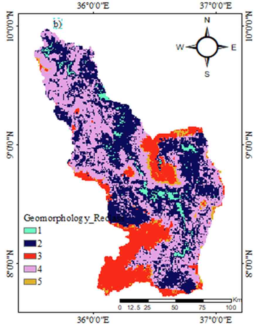
Geomorphology is the study of earth structures and landforms. It mainly depends on geological formation. From a geomorphological study point of view, the identification and characterization of diverse landforms and structural elements in the study region are very significant as they are required for groundwater potential. If the hydrogeological settings convey water for a geomorphological unit a slope based landform, low mountainous, and flat plains are markers for the presence of groundwater. The geomorphological map shows seven landform features namely: High altitude plains, Low plateaus, Mid altitude plateaus, High-altitude plateaus, Low altitude mountains, Mid altitude mountains, and High altitude mountains. These geomorphologies were reclassified into five units (Figure 9) as very poor = 1 (high mountains), poor = 2 (Hills), moderate = 3 (low mountains), high = 4 (plateaus), and very high = 5 (plains) based on the rate of groundwater recharge.
4.8 Lithology
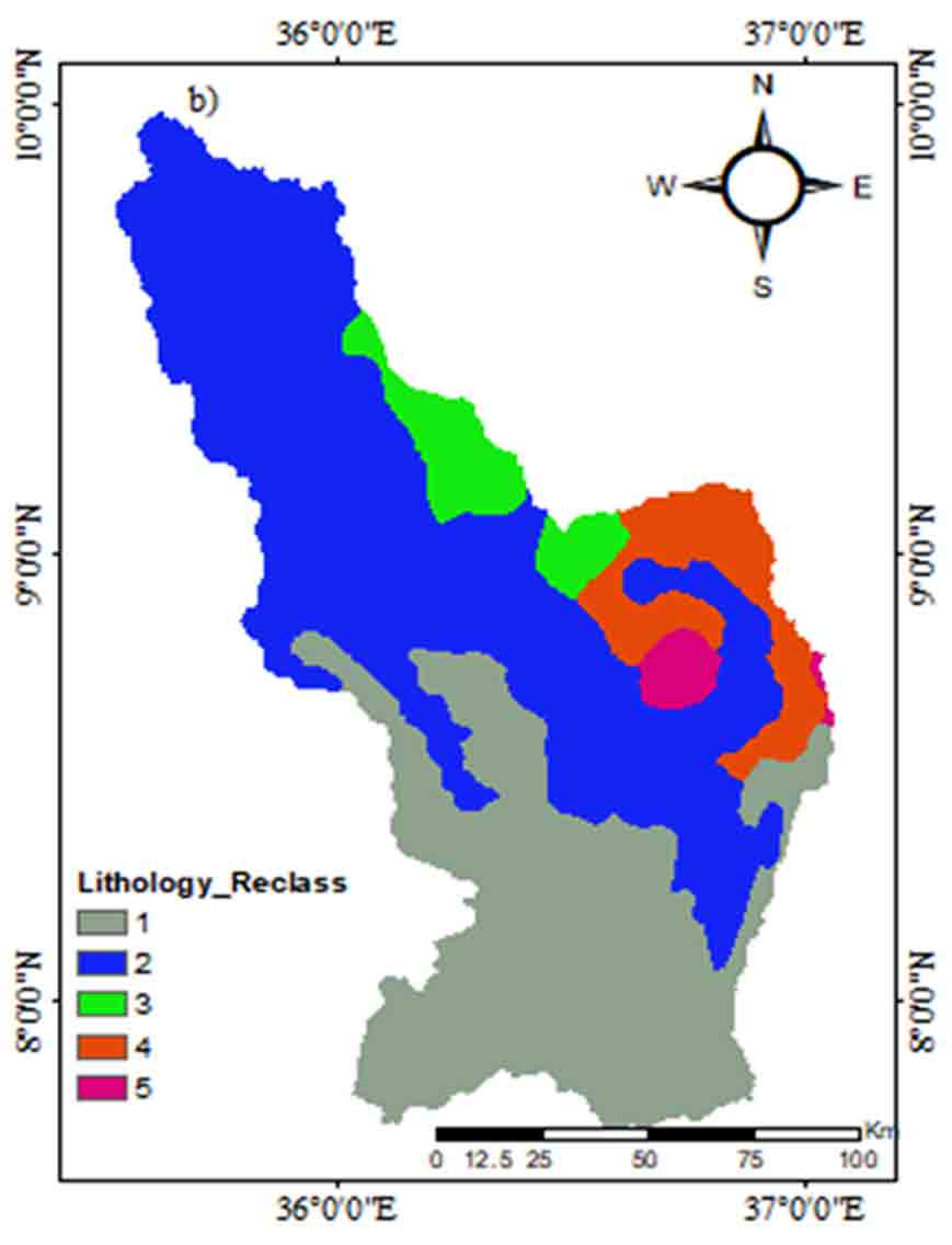
The presence of groundwater in an aquifer is determined by the geological settings’ lithology and permeability. Water is stored in the aquifer when the lithological formation holds and conveys the percolating water. The amount and volume of water stored in the geology is a function of the hydrogeological settings of the area. The water can only be stored if there are enough void areas between the geologic units. The aquifer is assumed to be potential when there are enough spaces in the hydrogeological settings. Porosity and permeability are frequently sufficient in lithological units with uniform grain sizes. Groundwater recharge occurs when precipitation from surface runoff lakes and streams percolates into the subsurface. The study area’s dominant lithology classes are Termeber, Adigrate Sandstone, Blue Nile Basalts, Marshsoils, Fluvium, Colluvium and Lateritecon Amba Alija Rhyolite, and the corresponding classes to the groundwater potential zones are very poor = 1, poor = 2, moderate = 3, high = 4 and very high = 5, respectively (Figure 10).
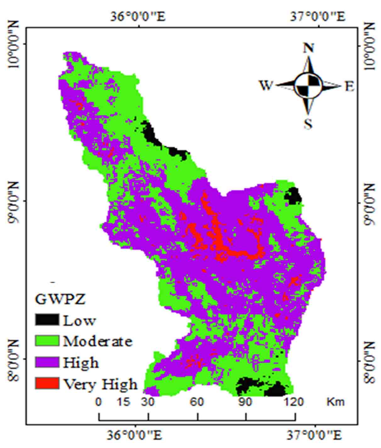
4.9 Groundwater Potential Zones
In locations like the Didessa Sub-basin, where rainfall is erratic, mapping the groundwater prospect zone is critical. Farmers in the study area are required to dig and construct bore wells in order to meet home water needs and maintain agricultural productivity through irrigation. The goal of this research was to find useful information and the optimum locations for groundwater investigation. Groundwater availability and distribution are always determined by a multitude of hydro-morphological conditions that affect soil infiltration and aquifer recharge (Hussein et al., 2016).
The groundwater potential zone map of the study area (Figure 11) was prepared through the integration of various thematic layers including rainfall and characteristics of terrain features such as geology, geomorphology, and slope. The entire watershed classified into very low, low, moderate, high, and very high groundwater prospect zones.
High groundwater prospect zone is widely distributed across most parts of the Subbasin. The total area covered by category is 66% (18532.2 km2) of the total area of sub-basin. The very high groundwater prospect zone is occupying 4.6% (1289.4Km2) of the area. This result is reveals with the findings by Wudad et al. (2021), Kindie et al. (2019), Melese and Belay (2021), Tamiru and Wagari (2021), Hussein et al. (2016), Debele (2020), Hussein et al. (2016), Bashe (2017) and Bawoke et al. (2020) who reported high infiltration and aquifer recharge rates in areas with flat slope, deep soil, and alluvial deposits. The river banks, wetlands and lake fringes of the Didessa Sub-basin also exhibited very good groundwater potential zones.
Appropriate weights were assigned to all thematic layers and their individual features after understanding their importance in influencing groundwater potential. Scores and weights were assigned to all thematic layers based on their roles in groundwater potential including infiltration, aquifer transmission, and storage. The scores and weights assigned to the individual features of the nine themes considered in this study are summarized in Table 4.
The analysis of thematic layers (rainfall, soil texture, slope, runoff depth, LULC, lineament, geomorphology, drainage density, and lithology) and the values of the parameters are given based on the Saaty scale as shown in Table 3. Based on the pairwise comparison matrix, the relative weight matrix and normalized Principal Eigenvector were calculated. The relative weight for thematic layers was assigned according to their relative importance.
The weights were normalized based on equation five (Equation 5), which are calculated by averaging the values in each row to get the corresponding ranking, which gives the results of normalized weights of each parameter as presented in Table 3. From the result, observed rainfall has the highest value rather than other parameters. Because, it indicates high rainfall has the possibility of high groundwater recharge thus high groundwater potential zones, while low rainfall indicates low groundwater recharge thus low groundwater potential zones. The main source of groundwater in the area was the rainfall of the northwestern and southeastern highlands in the study area due to mountain blocks and slopes.
The consistency index was computed to overcome for the formula of consistency ratio and this was done based on equation 9, which results in CI = 0.120. Then, the consistency ratio was computed as per equation 8 and the computed result of CR = 0.085 which is less than 0.1 and the given weights were valid for further analysis.The values of weights taken after the AHP analyses were used in the weighted overlay analysis for each criterion were fixed as 0.327, 0.242, 0.112, 0.1065, 0.0757, 0.064, 0.046, and 0.026 for rainfall, geomorphology, lineament density, drainage density, slope, soil, LULC, and lithology, respectively. Therefore, groundwater potential areas were obtained by the combination of all layers using the overlay analysis method in Arc GIS 10.7 (Equation 9):
\(GWPZ=32.76×Rf+24.22×Gm+11.18×Ld+10.65×Dd\)
\(+7.57×Sl+6.4×St+4.6×LULC+2.6×lith\) (9)
Rainfall, slope, lineament density, and geomorphology hold the highest value relative to the other parameters. The weight assigned for rainfall was greater than the weight of others, which influence the occurrence of groundwater potential and recharge zone than other parameters. The result indicated that about 2.1% of the study area classified (Figure 11) as low 27.35% classified as moderate, 66% as high potential, and 4.6% were classified as very high groundwater potential.
4 . CONCLUSION
In this study, the result of groundwater potential zones by using GIS and remote sensing techniques through AHP decision methods were identified and delineated based on the influential factors for groundwater potentials. Eight parameters were selected which have more affected the occurrence of groundwater potential zone before overlay analysis. It is possible to construct important criteria that have a stronger impact on the result than other criteria by applying quantitative weights. The AHP approach allows decision-makers to give judgments to reduce complexity in decision-making processes. The result of the consistency ratio in this study was 0.08 for the groundwater potential zone and the value was accepted for further analysis.
The delineated groundwater potential zones classified into four zones namely low, moderate, high, and very high. The low zone shows the low suitable area for groundwater prospects. A very high zone, on the other hand, indicates the best location for groundwater potential. The effective parameters in the area for groundwater potential zone are rainfall, slope, geomorphology, lineament density and drainage density in pairwise comparison matrix analysis indicates that all parameters are significant. The values of weights taken after the AHP analyses were used in the weighted overlay analysis for each criterion were fixed as 0.327, 0.242, 0.112, 0.1065, 0.0757, 0.064, 0.046, and 0.026 for rainfall, geomorphology, lineament density, drainage density, slope, soil, LULC, and Lithology, respectively. Therefore, groundwater potential areas were obtained by the combination of all these layers using the overlay analysis method in Arc GIS 10.7. The important factors result show that rainfall and geomorphology have a higher weight and lithology has the lowest weight for identifying the potential of groundwater in the study area. The result indicated that about 4.6% (1289.4km2) of the study area were classified as very high potential, 66% (18532.2km2) classified as high potential, 27% (7683km2) as moderate potential, and 2.1% (587.5km2) were classified as low groundwater potentials. This indicates that the AHP, GIS and Remote Sensing integrated approach for identification of groundwater potentials gives an acceptable result. Hence, it is fair to conclude that this result can be used for the planning of new groundwater based projects and expansion of the existing project in the sub-basin.