Keywords

Watershed , Terrain variables , Soil Properties , Random forest , Himalaya , Digital soil mapping

1 . INTRODUCTION

2 . STUDY AREA

The study was conducted in a small watershed of mid-Himalaya in Tehri Garhwal district of Uttarakhand state in India (Figure 1). The watershed is located at longitude of 78º 25ʹ 55" E to 78º 24ʹ 49" E and latitude of 37º 32ʹ 49" N to 30º 21ʹ 31" N covering an area of 196 ha. The elevation in the watershed varied from 1275 to 1925 m above MSL. The area is a micro-watershed falling within the Maniyar watershed, which drains to the Tehri dam reservoir. The watershed is dominantly covered with forest (especially pine, followed by agriculture and little scrub area. The climate, parent material and LULC were considered uniform throughout the study area due to very small spatial extent of the watershed.

Figure 1. Study area: (a) India, (b) Tehri Garhwal district of Uttarakhand and (c) soil sampling locations on a LISS IV false color composite (FCC) image

3 . MATERIALS AND METHODS

3.1 Data

CartoDEM version 2.0 having a spatial resolution of 10m, generated using Cartosat-1 stereo data was used in the study for generation of various terrain parameters (Table 1). The data was obtained from National Remote Sensing Centre, ISRO, Hyderabad. The DEM is reported to be high quality with vertical accuracy assessment yielding an RMSE value in the range of 3.6m to 4.4m and LE90 value of 7.2m (NRSC, 2014). The LISS IV image was used for generation of False Color Composite (FCC) image of the study area. 

3.2 Methodology

The watershed boundary was delineated from the DEM, using outlet location, employing the hydrology toolbox in ArcGIS. The DEM was pre-processed for the removal of pits. The pre-processed DEM was used to derive various terrain parameters i.e., elevation, slope(degrees), aspect, cos(aspect), sin(aspect), average curvature, plan curvature, profile curvature, flow direction, flow accumulation, heat load index, integrated moisture index, solar radiation, compound topographic index as well as stream power index of the watershed area.

3.3 Terrain Variables

Slope, a widely known primary terrain attribute, indicates the change in elevation or steepness of the surface with respect to a certain linear distance (Burrough, 1986). It plays an important role in defining the erosion rate as well as influences the pace of soil-forming processes at a particular location and thus contribute significantly in defining the spatial distribution of soil properties. Aspect indicates the direction of the steepest slope/downslope of a particular location. It is mainly measured clock wisely from north (0º-360º). The aspect plays a significant role in determining the vegetative growth in the area as well as the rate at which pedogenic processes and soil erosion operates. Sin(aspect) and Cos(aspect) are transformations of aspect done mainly to avoid use of circular data. Instead, the transformations will help us to have a measure of northerness (cosine transformation) and easterness (sine transformation). Flow direction is primary terrain parameter, which indicates the direction in which flow will occur from each cell in a raster. The direction is determined based on the steepest descent, or maximum drop, from each cell, to its neighboring or surrounding cells. Flow accumulation indicates accumulated flow of a cell as the accumulated weight of all cells flowing into each downslope cell. The flow accumulation value denotes the number of cells that flow into each cell. Compound Topographic Index (CTI) a widely used secondary terrain index was computed as per equation (1) making use of average upstream contributing area (As) and slope gradient (β) (Moore et al., 1993). It helps to quantify the involvement of topography on soil erosion occurring in a specific location. CTI also referred as Terrain Wetness Index (TWI) describes the spatial arrangement and extent of soil saturation zones as well as variable sources for run-off generation. Lower CTI values generally depict upper catenary/slope positions whereas lower positions are represented by larger values (Jenson, 1991).

\(CTI = In\left(\frac{A}{tan \beta}\right)\)                     (1)

where, As indicates the upstream contributing area in m² and β, the local slope gradient.

Stream Power Index (SPI) is a commonly adopted secondary terrain parameter especially in hilly terrains. It reflects the erosive power of a terrain and provides an idea about the rate of dissipation of energy by flowing water on the channel bed and basins and aids to determine potential strength of flowing water to stimulate erosion and sedimentation. Higher value of SPI indicates chances of higher erosion rates in an area. SPI computation as per equation (2) is based on the idea that discharge quantity is directly related to its contributing catchment area (Jenson, 1991).

\(SPI=ln⁡(A \times tan⁡β)\)             (2)

where, A indicates the upstream contributing area in m² and β, the local slope gradient.

Curvature is the second derivative of a surface and is computed as slope of the slope. The curvature outputs are helpful in describing the physical characteristics of a drainage basin with the aim of understanding runoff and erosion processes. Profile curvature is calculated in a direction parallel to the maximum slope, whereas plan curvature is in a direction perpendicular to it. The values indicate whether the surface is upwardly convex, upwardly concave or flat/linear at cell depending on the values (negative, positive or zero). Profile curvature values influence the acceleration and deceleration of flow and thereby influence erosion and deposition processes, whereas convergence and divergence of flow across a surface is regulated by plan curvature. Heat Load Index (HLI) generated using the method given by McCune and Keon (2002) signify temperature variations between different slope directions by means of ‘folding’ the aspect. In doing so, the highest values of the index are assigned to southwest and the lowest to northeast aspects. The index is based on the concept that while Potential Direct Incident Radiation (PDIR) is found to be symmetrical along the north-south axis, temperatures are not. This is because a slope experiencing afternoon sun was found to have higher maximum temperatures than a similar slope with morning sun (McCune and Keon, 2002). As a result, slopes facing southwest direction would be much warmer compared to a southeast facing slope, even though both receive equivalent amount of solar radiation. In addition, this index takes into account steepness of slope, which many other aspect-rescaling equations fail to do (McCune and Keon, 2002). Integrated Moisture Index (IMI) helps to integrate the GIS-derived topographic and soil features of the landscape into a single index. A wide variety of ecological processes operating at landscape levels are found to be statistically related to IMI (Iverson et al., 1997).

      \(IMI=(HS.0.40)+(FA.0.30)+(C.0.10)+(TWHC.0.20)\)      (3)

The value of IMI ranges between 0 and 100, where higher values indicate high relative moisture status. It offers a relative rating of moisture using four inputs namely hill-shade, flow accumulation, curvature and total water holding capacity. The values of all input variables are scaled; scores brought to the range of 0 to 100 and further multiplied with their corresponding weights as per equation (3) to estimate IMI. The solar radiation parameter calculates insolation across specific locations or a landscape, adopting procedures from the hemispherical view-shed algorithm (Rich et al., 1994; Fu and Rich., 2000; Fu and Rich, 2002). The analysis yields a solar radiation product (Wh/m²), indicating the total amount of radiation calculated for a particular location or area. The solar radiation analysis facilitates analysis and mapping of solar effects over a geographic area for specific periods. It can account for atmospheric effects, elevation, slope, aspect, latitude, daily and seasonal shifts of sun angle, and shadow effects by neighboring topography. The resultant outputs can assist in physical and biological process’ modeling due to their easy integration with various GIS data (ESRI, 2011).

3.4 Soil Sampling

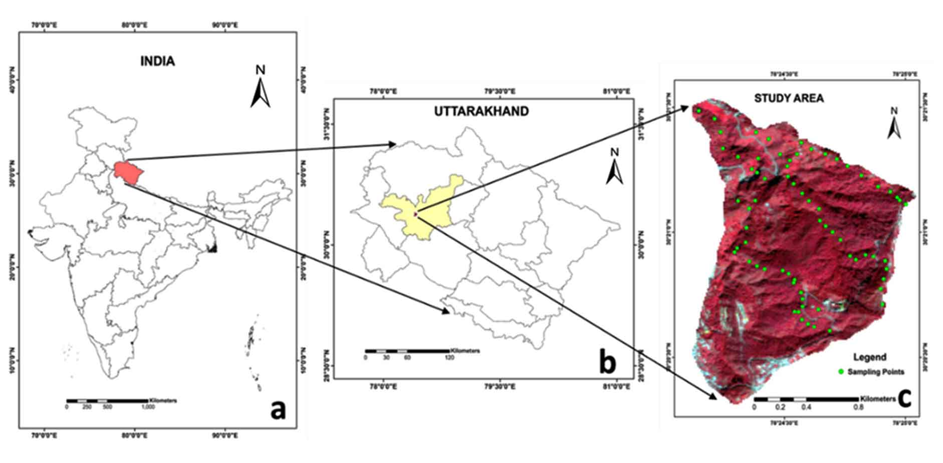
Transect sampling approach was used for soil sample collection from the study area, as the steep sloping terrain was difficult to traverse and ruled out the possibility of grid sampling. Transect sampling was done taking special care to cover the entire elevation range within the watershed. Field data collection in the study area was done by collecting soil samples from 0-15cm depth (surface layer) at 68 different locations following a transect survey method. Handheld GPS (Trimble Juno SD) was during field sampling for recording precise geographic coordinates of sampling locations in the various transects covering entire elevation range in the watershed. The collected soil samples were securely packed and correctly labeled in polythene bags, and transported. The samples were then subjected to air-drying in the laboratory and sieved using a 2-mm sieve for removing small pebbles as well as root/litter particles.

3.5 Estimation of Soil Properties

TOC Analyzer (Shimadzu TOC-VCPH) was used for determination of total soil carbon in the soil samples, using 0.2mm sieved samples, after air-drying and homogenization. Similarly, total nitrogen content of the samples were estimated using CHNS analyzer (Elementar vario MACRO cube). Soil textural composition (percentages of sand, silt and clay) was estimated using Bouyoucos hydrometer method (Bouyoucos, 1962) after dispersing the soil samples using sodium hexametaphosphate in solution.

3.6 Random Forest Modeling

The random forest regression model (Breiman, 2001), a non-parametric technique was developed by extending the Classification and Regression Trees (CART) program with the aim of improving the model’s prediction performance. It uses randomness and bootstrap samples in the tree building procedure. The model is a combination of several trees simulating the concept of forest which act as predictors and the results derived from the model represents the mean of predictions/results obtained from all trees forming/comprising the forest (Breiman, 2001).

Random Forest (RF) package in R software (R Development Core Team, 2007) was employed for implementation of RF model in the study. Model fitting was decided by three parameters viz., the number of trees in the forest (n_tree), the minimum number of predictors used per tree (m_try), and the minimum number of samples per terminal node (node size; n_min) (Liaw and Wiener, 2002). The standard n_tree value of 500 defined in the package was used in this study. Node size value of five and m_try value of four was used. Out-of-bag (OOB) mean square error and the percentage of variance explained by the model were used for evaluating the efficiency of RF modeling for spatial prediction of various soil properties.

The developed models’ performance is evaluated by means of an independent dataset referred as validation data set, which was not involved in calibration or model development. The soil dataset of 68 points were split randomly into two, one used for calibration (46 points) whereas validation was done using the other (22 points). The model performance was evaluated based on coefficient of determination (R²), Root Mean Square Error (RMSE) as well as Lin’s Concordance Correlation Coefficient (CCC) values generated using validation dataset, based on observed and estimated values of each soil property. Lower the RMSE value, higher the accuracy of prediction. The validated models were further used for mapping the spatial distribution of different soil properties in the study area.

4 . RESULTS AND DISCUSSION

4.1 Soil Properties

Descriptive statistics of various soil properties addressed in this study (both calibration and validation datasets) are shown in Table 2 and Table 3. The results indicated that both calibration and validation datasets are having very similar mean values for all the soil properties with no significant difference in the various soil properties at 95% confidence interval based on the results of analysis of variance (ANOVA). The total data set had mean values of 38.63%, 39.93%, 21.62%, 2.37 gkg^-1 and 0.18% corresponding to sand, silt, clay, total organic carbon and total nitrogen, respectively (Table 2).

Both the sample sets were found to be highly heterogeneous, indicated by higher values of coefficient of variation (CV). The CV values varied from 17.92 to 45.25 % in case of calibration dataset, whereas it varied from 26.64 to 80.62% in case of validation dataset. The nitrogen content exhibited highest CV values followed by carbon in both the sets, indicating the increased variability of these soil properties in the watershed. This higher variability may help us in getting better prediction results as reported by Dematte et al. (2007).

4.2 Relationship with Terrain Variables

The correlation analysis revealed the nature of relationship between different soil properties and various terrain parameters (Table 4). Flow direction, heat load index and solar radiation were found to be significantly correlated with sand content in the study area. The above mentioned three parameters along with an aspect were found to be significantly correlated to silt content. Elevation and aspect were found to have significant inverse relationships with TOC content as well as nitrogen content (Table 4). Dharumarajan et al., 2017 have also reported similar inverse relationships. The absence of significant relationships indicates the nonlinear nature of relationship various soil properties are having with terrain variables.

4.3 Performance of Random Forest Modeling

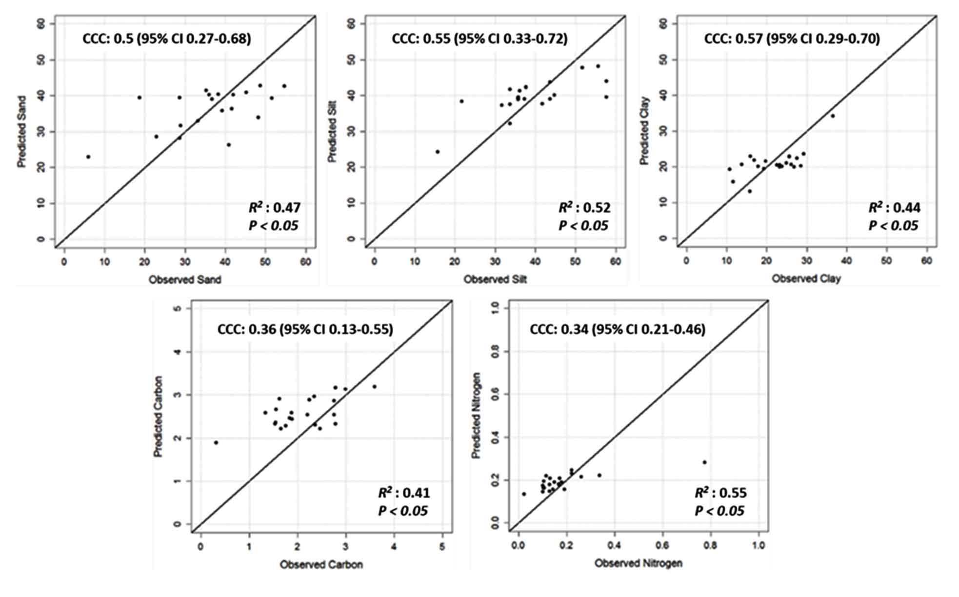
The performance of random forest modeling for prediction of various soil properties using terrain variables were evaluated using various uncertainty indictors viz. R², RMSE and Lin’s CCC. The results revealed that models generated using various terrain parameters could explain 47%, 52%, 44%, 41% and 55% of the variation for sand, silt, clay, carbon and nitrogen, respectively (Table 5; Figure 2). Lin’s concordance correlation test revealed that clay exhibited the highest CCC value (57%) whereas nitrogen exhibited the lowest CCC value (34%). The RMSE values were found to be 11.02, 7.51, 4.75, 0.73 and 0.12 for sand, silt, clay, carbon and nitrogen, respectively (Table 5). The models developed were found to be low to moderately satisfactory for predicting various properties.

Figure 2. Concordance correlation coefficient plots of different soil properties

Among the various models generated, RF models for prediction of particle size fractions were found to have higher predictive performance (indicated by LCCC values >0.5) in comparison to organic carbon and nitrogen contents. Attempts to predict spatial distribution of soil properties solely based on terrain parameters is very rare and less reported. Ließ et al. (2012) has reported the use of DEM derived terrain parameters as covariates for RF modeling. They reported prediction models that can explain 30-40% of the variation in soil texture, which was lower than the results obtained in this study (Table 5). Similarly, Akpa et al. (2014) reported Random Forest Models (RFM), which explained 48-49%, 26-27% and 53-56% of variance for sand, silt and clay respectively in surface layer. Their outcomes are in agreement with our findings for sand, poor in comparison to silt and better in case of clay. Similar or less accurate prediction results with respect to sand, silt and clay have also been reported by various researchers (Hitziger and Ließ, 2014; Vaysee and Lagacherie, 2015; Chagas et al., 2016).

The developed models were able to account for around 50% variation only of different soil parameters. The inability to account for the rest 50% variance may be due to the different factors like tree height, storied growth, boulders, coarse fragments, embedded deposits etc., which cause intra terrain variations in flow and transport of materials. The intra-terrain variability may have caused lower accuracy as the slopes here are not characterized as smooth slopes, which cause limitations in accounting for the impact of terrain on material transport (comparative erosion/deposition processes operating in slopes at small scale).

The performance of the developed models for organic carbon and nitrogen were found to be lower than that of the models for particle size fractions (Table 5). The prediction performance of models for organic carbon in this study was found to be high in comparison to the results obtained by de Carvalho et al. (2014) (R² = 0.20), Gastaldi et al. (2012), (R² = 0.18) and Dharumarajan et al. (2017), (R² = 0.23). The comparatively better results in this study may be attributed to the higher sampling density (34.69 samples per km²), coupled with the use of high spatial resolution (10m) covariates for modeling, which can capture the local scale variations occurring along the slopes in the hilly terrain more efficiently. Still the results were poor in comparison to the works reported by Wiesmeier et al. (2011), Guo et al (2015), Vagen et al. (2016), Sreenivas et al. (2016) and Kalambukattu et al. (2018) who have reported R² values of 0.76, 0.69-0.77, 0.82 and 0.83, respectively for organic carbon predictions. This may be due to the inclusion of various continuous as well as categorical environmental covariates corresponding to different factors of soil formation. In case of nitrogen even though R² value was above 0.5, the Lin’s CCC value (0.34) was found to be the lowest among all the variables. The approach adopted in the study may be useful for soil properties prediction in areas with similar terrain conditions.

4.4 Importance of Variables

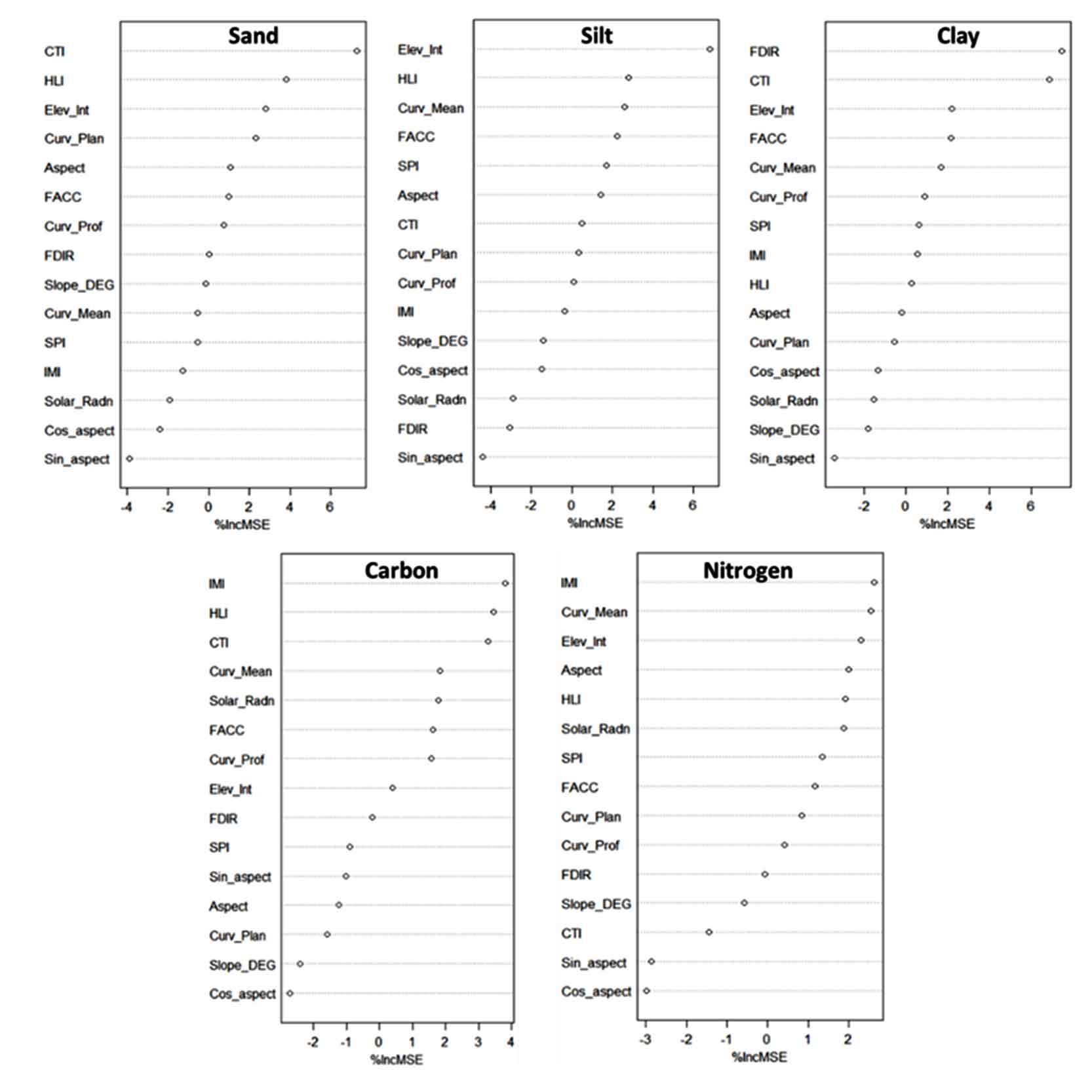
The relative importance of various input parameters for modeling can be estimated using RF model, an advantage over various other modeling approaches (Cutler et al., 2009). In addition, the RF modeling aids us in avoiding the elimination of various predictive variables (even if they are correlated), which may be significant with respect to specific properties (Akpa et al., 2014). In RF modeling, the variable importance is estimated based on how good or bad the model predicts, if one or few variables are removed (Prasad et al., 2006). It also safeguards good predictor variables from being eliminated and preserves them for model.  Variable importance rankings of RF models generated for spatial prediction of sand, silt, clay, organic carbon and nitrogen are given in Figure 3. CTI was observed to be the most important variable for prediction of sand, followed by HLI, elevation and plan curvature. The most important variables for modeling and prediction of silt content were elevation > HLI > mean curvature > flow accumulation, whereas for clay, the most relevant variables were flow direction > CTI > elevation > flow accumulation. For organic carbon the important variables were IMI > HLI > CTI > mean curvature, and for nitrogen, IMI > mean curvature > elevation > aspect. These results clearly confirm that the relative importance of various predictor variables is dependent on soil property under consideration along with other variables. The lower percent increases in mean square error (% IncMSE) values may be improved by the inclusion of various other environmental covariates corresponding to different factors of soil formation, in addition to the terrain related covariates as well as more detailed soil samples (Akpa et al., 2014). Various terrain parameters governing the spatial distribution of soil properties could be identified during the study, which may be quite useful in future studies, for understanding the influence of terrain on soil properties.

Figure 3. Variable importance plot/rankings of the environmental covariates generated using RF models for sand, silt, clay, organic carbon and nitrogen.

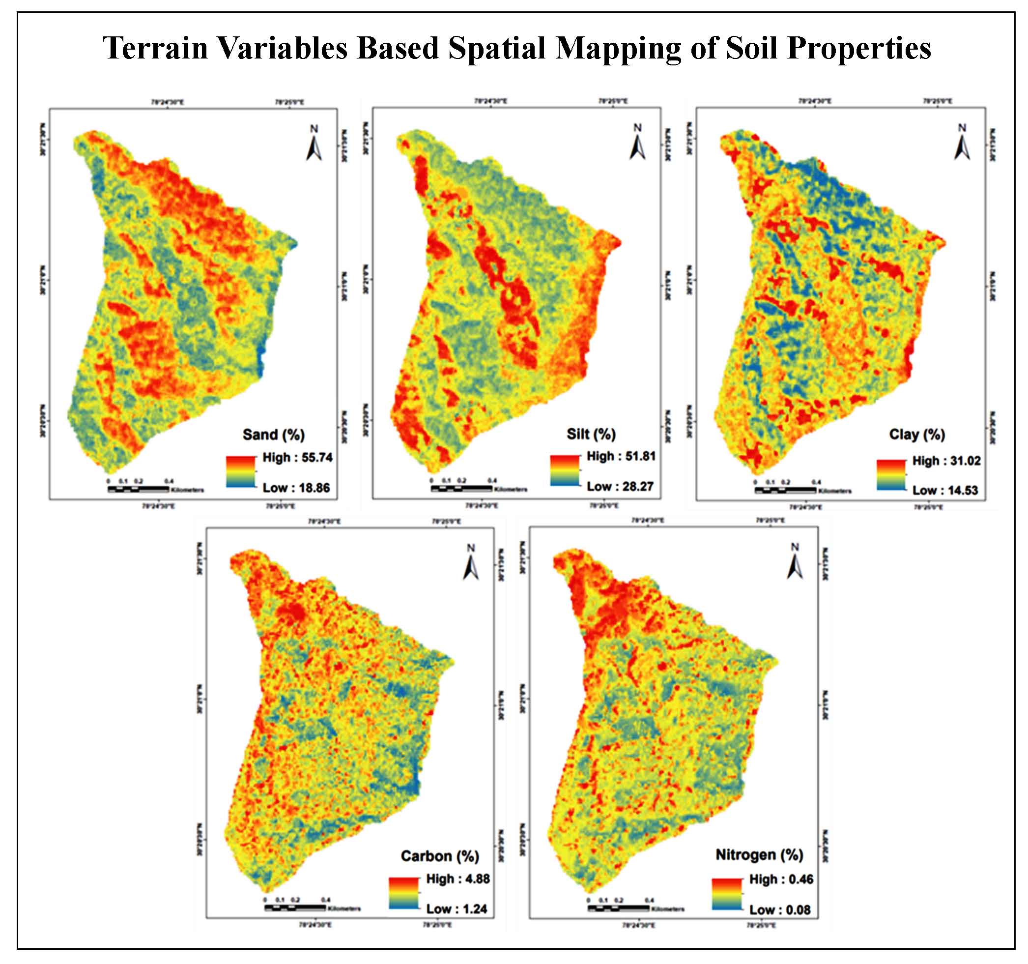
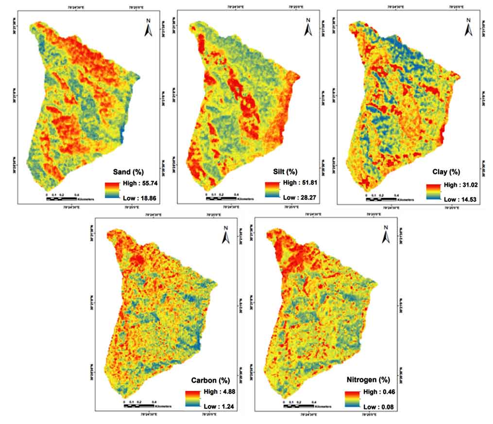
4.5 Spatial Mapping of Soil Properties 

Spatial distribution maps of various soil properties were generated using the validated RF models (Figure 4). The predicted sand content ranged from 18.86-55.74%, the clay content varied from 14.53-31.02%, whereas silt content varied from 28.27-51.81% in the area (Table 6). The soil carbon and nitrogen contents ranged from 1.24-4.88% and 0.08-0.46%, respectively (Table 6). The Skewness values of different properties indicted that the values are symmetrical (sand, clay, carbon) to moderately skewed (silt, nitrogen). Symmetrical distribution indicates that the predicted values followed a normal distribution, whereas the moderate Skewness indicates the predominance of predicted values in the lower range.

Figure 4. Predicted spatial distribution of different soil properties using RF model

The spatial distribution of primary soil particles (sand, silt and clay) as well as soil nutrients (soil carbon and nitrogen) showed large variation in their contents which is governed by the variations in terrain variables. The terrain characteristics play the most vital role in governing the transport and deposition of materials in these hilly mountainous ecosystems. The improved contribution of IMI as well as HLI in prediction of carbon as well as nitrogen may be attributed to their significance in influencing the micro-variations in temperature as well as moisture distribution at landscape level. These moisture as well as temperature variations can influence the decomposition and other biochemical changes for these nutrients in addition to the physical material transport processes of erosion and deposition. Several researchers have reported similar role of moisture regimes in influencing distribution of various soil properties (Hairston and Grigal, 1994; Gessler et al., 1995; Morris and Boerner 1998). Application of various advanced techniques suggested by various researchers such as wavelet transforms, neural networks, support vector machine, additive regression etc (Kalambukattu et al., 2018; Pande et al., 2022; Elbeltagi et al., 2022) for soil properties prediction and mapping may also be explored for improving the accuracies in such difficult terrains. The maps of sand, silt and clay may be used for identifying the various zones of erosion and deposition, which will help in improved planning as well as implementation of various soil and water conservation measures in the watershed. Carbon and nitrogen maps may also help us in identifying areas with soil fertility constraints as well as degradation risks. This will aid in planning and implementation of various management practices ultimately leading to improvement in sustainable agricultural production.

5 . CONCLUSION

Tables

Figures

Conflict of Interest

Acknowledgements

Abbreviations

References