Geo-economic Feasibility of Apple Orchards Across Physiographic Divisions in Kashmir Valley, India

Volume 6 (2022), Issue 1, Pages 40-48

Journal of Geographical Studies

ISSN : 2582-1083

DOI : http://dx.doi.org/10.21523/gcj5

Original Research Paper

Geo-economic Feasibility of Apple Orchards Across Physiographic Divisions in Kashmir Valley, India

Fayaz A. Lone ³

, Showkat A. Ganaie ¹

, M. Imran Ganaie ²

, M. Shafi Bhat ³

, Javeed A. Rather ³

1.Department of Geography, Govt. Degree College, Shopian-192303, Jammu and Kashmir, India.

2.Department of Geography and Disaster Management, University of Kashmir, Srinagar-190006, India.

3.Department of Geography, University of Kashmir, Srinagar-190 006 (India).

Author for Correspondance : Mr.M. Imran Ganaie^*

*.Department of Geography & Disaster management, University of Kashmir, Srinagar-190 006 (India).

Proccessing Editor : Professor.Masood Ahsan Siddiqui¹

1.Department of Geography, Jamia Millia Islamia – A Central University, New Delhi-110025 (India).

DOI : https://doi.org/10.21523/gcj5.22060103

Article History :

Date of Publication : 15-08-2022

Date of Submission : 03-07-2022

In Final Form : 01-08-2022

Date of Acceptance : 02-08-2022

Graphical Abstract

Highlights

The present study focussed on analysis of economic feasibility of apple cultivation in different physiographic divisions.
The study is based on primary survey conducted in all physiographic divisions.
Better economic returns estimated for Karawas division.
The study facilitates for area-specific strategy development with wider recognition of different altitudes.

Abstract

Financial investments in apple cultivation in Kashmir valley are increasingly recognized as key drivers of economic growth and employment creation. This paper presents a comprehensive economic analysis across physiographic divisions using precise economic indices that include cost-benefit analysis, project evaluation method and other socio-economic determinants. It relies on a primary survey of 866 farm-households selected across four physiographic divisions of the Kashmir valley viz- valley floor, karewas, foothills and side valleys. Results reveal that the karewas fetch the highest returns from an investment owing to its ideal geographical conditions. On contrary, the non-karewas belt was found to be trailing in one or more economic indices although the financial feasibility of investment in apple cultivation was still found satisfactory. The study affirms that agricultural land-use decisions at the micro-scale should be determined by the site-specific attributes and that economic indices are largely dictated by physical characteristics of land itself. While demonstrating the utility of land-use decisions in light of geographical factors, our results can assist both farmers and policy-makers to design a more adapted land use strategy for fostering financial investments in apple cultivation in the valley.

Keywords

Profit , Physiography , Karewas , investments , Apple

1 . INTRODUCTION

Apple plantation has emerged the most dominant land use in the Kashmir valley, absorbing mostly fertile agricultural landscapes in non-kerewa belt in the recent past (Alam et al., 2019; Ganaie et al., 2017; Bhat and Shah, 2011; Wani et al., 2009). The horticultural sector in the study area has witnessed a phenomenal growth of 17.5% in its area from 1980 to 2014 (Malik et al., 2017; Ganaie and Bhat, 2014) and accounts for 2 million metric tonnes, contributing 67.7% of total apple production in the country (Shafi et al., 2019). The apple industry contributes overall economic activity of $2 billion equivalent to 10% of total economy of Jammu and Kashmir provides 150 million labor days annually during production process alone. The significance of apple cultivation in the valley is realized by the fact that the valley of Kashmir has more area under apple crop than the United States (the world’s second-largest producer of apples) and ranks sixth in the production of apples in the world (Haseeb, 2020). Despite having tremendous potential for apple industry, economic feasibility assessment, especially for commercial crops, is prelude to achieving sustainable productivity output in the valley of Kashmir. Economic feasibility evaluation of a land unit for a specific land-use can provide a more reliable prediction of land performance since land-use decisions are more based on economic value than physical evaluation (Dent and Young, 1981; Rossiter, 1995). Nevertheless, it is still a prerequisite to identify the land potentials and constraints, which otherwise would result in considerable productivity differences across spatial units in conformity to differences in biophysical and land qualities (FAO, 1976; FAO, 1983; FAO, 1995; Barlowe, 1978). Therefore, the decision-making process based on economic feasibility assessment must inherit an interdisciplinary character (Sojkova and Adamickova, 2011). Measures of economic feasibility evaluation include cost-benefit ratio, gross income, net income, net present value, internal rate of returns, pay-back period, utility functions and so on (Rossiter, 1995). Most of the studies related to financial feasibility and economic evaluation of crops are based on cost-revenue methods since annual crops don’t require evaluation of time value of money (Selvavinayagam, 1991). However, cost incurred on a perennial basis is virtually a project owing to its long life cycle and therefore, involves evaluation of many economic indices that serve as an important yardstick to judge economic performances (DeJong et al., 1999; Reganold et al., 2001; Sojkova and Adamickova, 2011; Badiu et al., 2015). In other words, an apple orchard is a long-term financial initiative that requires an appropriate procedure to evaluate investment decisions (Bechtel et al., 1995). The ideal and most appropriate methodology for this purpose is net present value to arrive at best possible assessment outcomes (Tauer, 2002; Cicek et al., 1999).

Sufficient studies have been conducted on economic feasibility of investments in apple orchards globally (Sultanov, 2021; Sojkova and Adamickova, 2011; Robinson, 2013). However, the majority of them have studied apple orchards from technological perspective neglecting the land qualities which are very critical for success of such investments. In Kashmir valley, no single study on the financial feasibility of apple orchards has been ever addressed despite the significant economic potential of apple production in the region. Also, farmers in the last three decades are continuously shifting their agricultural land especially paddy fields into orchards in non-karewa belts without assessing the biophysical suitability of the land concerned (Ganaie et al., 2017). In this scenario, the research question here is how far the expansion of apple orchards in other physiographic divisions is efficient. This becomes more relevant as the investment cost is very huge and involves a period of 40 years. Besides, investment cost in apple orchards is irreversible and pose potential risk of total financial failure. Importantly apple growers in the valley with small land holdings don’t have sufficient financial strength to cope with monetary losses. Thus, the present study was conducted to explore economic feasibility of apple orchards across physiographic divisions so that a linkage between biophysical and economic parameters is demonstrated more comprehensively. Such an endeavor would fill a research gap that could facilitate in decision-making related to land use planning and horticultural development in the study area.

2 . STUDY AREA

The study area lies between 33º30'N to 34º40'N latitudes and 73º45'E to 75º35'E longitudes and stretches over an area of 15,853km². Kashmir valley is one of the three meso-regions of the erstwhile state of Jammu and Kashmir that are isolated from one another by the Himalayan mountain ranges. It has been said that these divisions are like a three-story building in the midst of which is the Kashmir valley, which has a semi-closed ecosystem (Raza, et al., 1978; Dar, 2017; Khan, 2007). Being geologically an intermountain basin, the Kashmir valley is bounded by the Greater Himalayas to the northeast and the lesser Himalayas (Pir Panjal range) to the southwest (Romshoo et al., 2020). The Kashmir valley comprises of ten districts, which is 140km long from North to South and 45km wide from East to West (Ganaie and Bhat, 2014).

Figure 1. Study area: South Kashmir (India)

The valley of Kashmir can be divided into the following sub-categories based on physiographic distinctions: the valley floor, the karewas, foothills or rimlands and side valleys (Lone et al., 2022; Singh, 1971). The valley floor is its most notable feature, composed of alluvium deposited by Jhelum River and its tributaries. Due to leveled terrain and the abundance of fertile alluvial deposits, irrigational facilities are available throughout the year. Paddy fields predominate the agricultural landscape, which is referred to as the “rice bowl of Kashmir”. Karewas are a significant physiographic feature of the Kashmir valley, just like the valley floor. The Karewas are flat-topped, lacustrine-derived mounds with an undulating surface that surround the valley floor on both sides (Kumar et al., 2020; Bhatt, 1975). Along the valley’s longitudinal extent, they spread across a sizable portion of the southern edge. Around mountain ridges, they tend to slope, and at the valley’s center, they have a relatively flat top (Lone et al., 2022). These characteristics make them perfectly suited for horticultural pursuits. The foothills are mostly border mountains and the low-lying mountainous region of the valley (Easterbrook, 1999; Juanico, 1987). These hills are covered in a dense canopy of conifers that extend from the diverse Himalayan mountain ranges down to the valley plain. The side valleys constitute geographically the major tributary regions of the Jhelum river (Sabha et al., 2020), which exhibit various micro-scale geomorphic and climatic changes and provide the area with yet another distinctive agro-ecological regime.

3 . MATERIALS AND METHODS

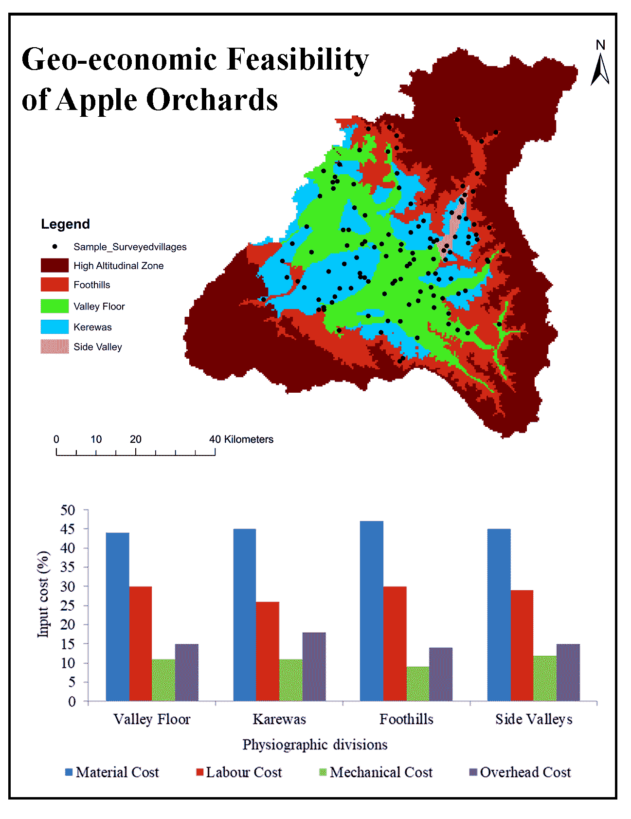
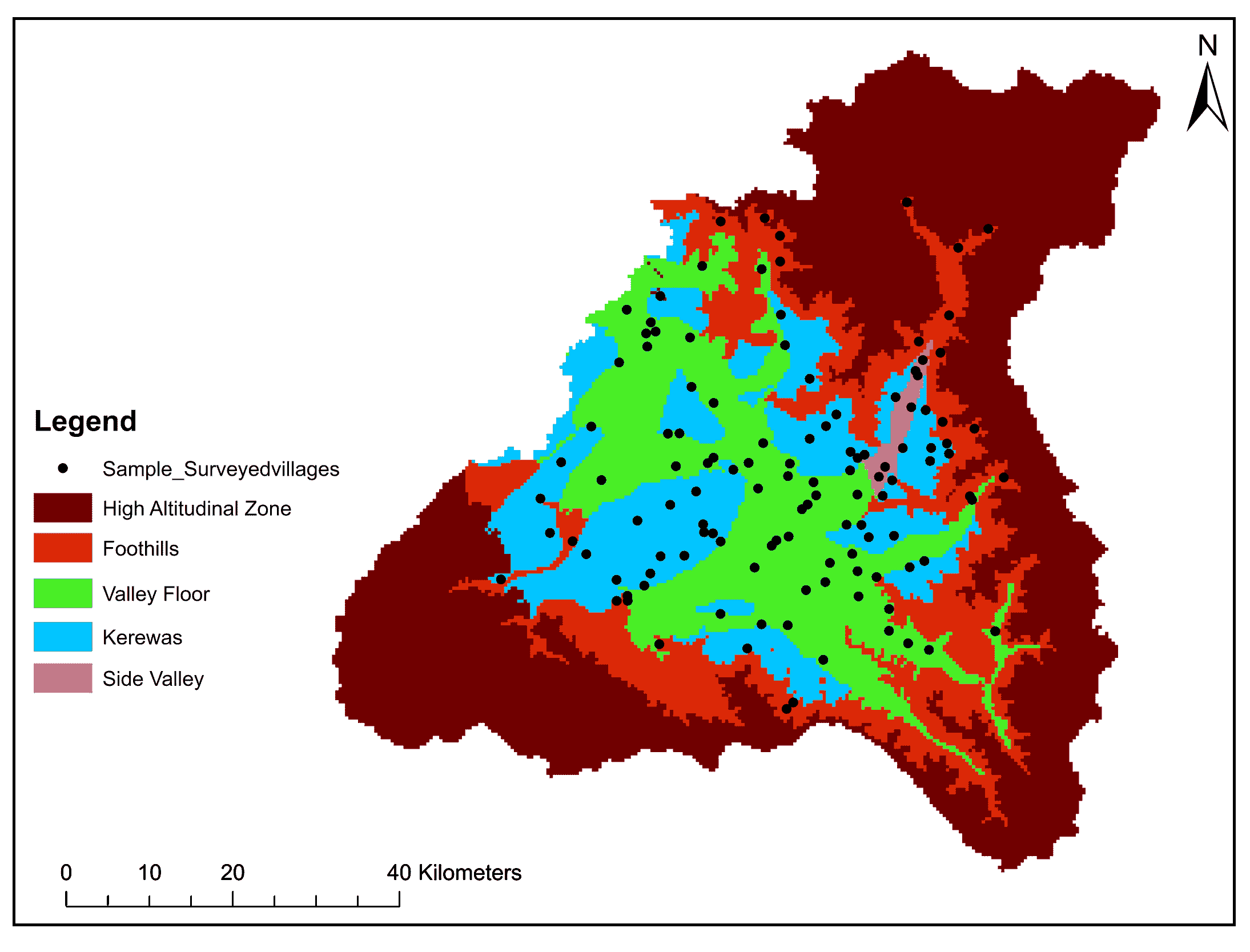
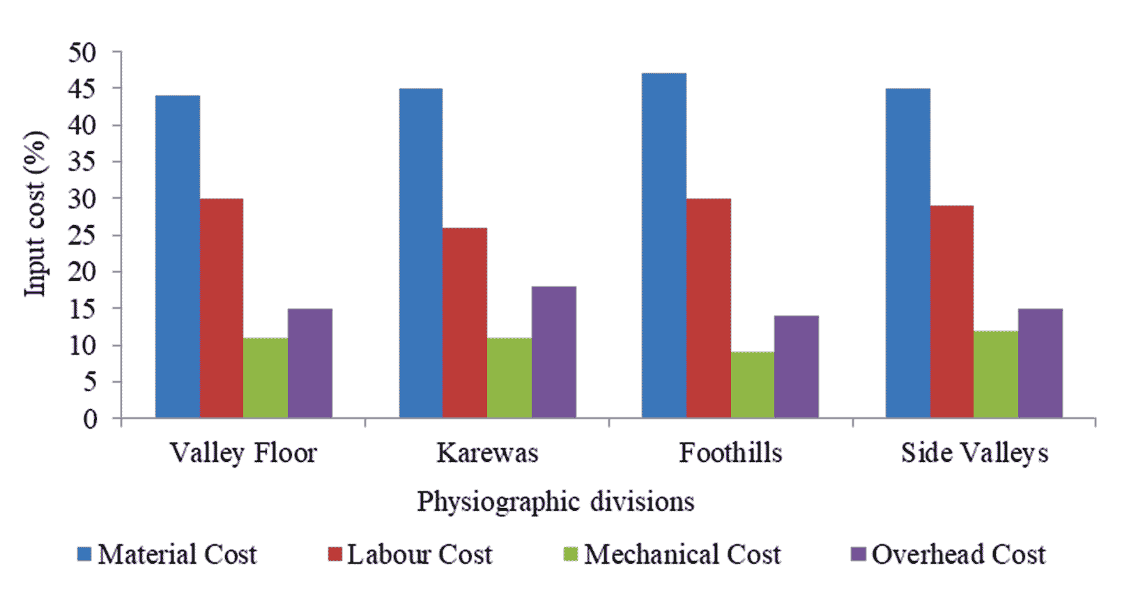
The study employed data from both primary and secondary sources. Primary data were collected in order to estimate the input and output cost empirically. For sampling purpose, the South Kashmir region of the Kashmir valley was specifically chosen because it has predominant horticulture, allowing for more reliable study results. South Kashmir is divided into four administrative districts: Anantnag, Pulwama, Kulgam, and Shopian (Ganaie et al., 2022a, 2022b). Moreover, this region has high agricultural and horticultural development (Ganaie et al., 2014). A basic unit of land measurement in the research region is the kanal’ (0.05 hectare), on which the analysis was based. The study area was delineated into four physical divisions, viz, valley floor, karewas, foothills and side valley. The physiographic map was generated using SOI toposheets on a 1:50000 scale a digital elevation model (DEM) and geological maps of karewas, as well as comprehensive field observations for ground verification and post-processing. The villages that fell inside each physiographic zone were identified by superimposing the village map over the physiographic map to determine the sample locations (Figure 2).

Figure 2. Sampling locations

In each physiographic zone, 10% of the villages were randomly selected, and 2% of the farm-operating households in each village were administered a survey for sampling. This led to the generation of 866 surveys at the farm-household level, divided into four physiographic groups. The data was collected pertaining to all the costs incurred on apple orchard starting from its establishment to the production and marketing stage. Based on data provided by apple farmers, the annual mean during the fructification stage was used to calculate the level of output and the price per unit. The evaluation of economic feasibility of an apple orchard involves a complex set of indices that cover various aspects of investment appraisal (Badiu et al., 2015). The life of an apple orchard in the study area is around 40 years (traditional orchard system). As such the methodology must include the time value of money. In the present study, we are employing widely used investment appraisal methods viz. net present value (NPV), internal rate of return (IRR), and payback period (Sojkova and Adamickova, 2011). Besides, cost-benefit ratio and descriptive statistics were also employed for data analysis.

3.1 Net Present Value (NPV)

Any economic venture, including a crop, is said to be viable if the predicted additional gain surpasses the total input costs incurred during the production phase. Any perennial crop such as apple involves time and calculating aggregate cash inflows occurring in subsequent years require adoption of appropriate discount rates to calculate the present value of future flows. Indeed, this is one of the guiding principles since discount rates should accurately reflects the opportunity cost of the capital to permit a comparison of the value of money in different periods. The net present value is calculated by the following mathematical expression (Erkus and Rehber, 1998):

$NVP = \sum^n_{t=1} {(Bt-Ct) \over (1+r)t} -I_t$

Where

$Bt$ = benefits at time t, $Ct$ = cost at time t,

$I_t$ = investment cost, n = project economic life,

r = discount rate

In our study, the net present value was calculated at the discount rate of 7.5% which also represented the opportunity cost of capital.

3.2 Internal Rate of Return (IRR)

IRR is the discount rate that produces zero NPV. Therefore, it is equivalent to the discount rate r that satisfies the following relationship (Badiu et al., 2015):

$NVP = \sum^n_{t=1} {(Bt-Ct) \over (1+r)t} =0$

where, Bt is the benefit stream and Ct is the cost stream.

The economic activity (an apple orchard in our case) is profitable if IRR is greater than the interest rate that could be earned in alternative investments; thus when IRR > ‘r’ the activity is considered viable. If ‘r’ also called opportunity cost of capital is lower than the IRR, then NPV is positive and vice-versa. This is expressed as:

$IRR>r=I^{mkt}=NPV>0$

$IRR<r=I^{mkt}=NPV<0$

3.3 Payback Period

Taking the changing value of money into consideration, the payback period is defined as the period (years) for which the discounted net cash inflow will cover the discounted value of each investment. The payback period of a project satisfies the following relationship (Badiu et al., 2015).

$Payback \ period = \sum^n_{t=0} {I_k \over (1+i)t} =\sum^n_{t=0} {NI_k \over (1+i)t}$

where,

$I_k$ = Value of investments in the k^th year

$NI_k$ = Net income of the activity in the k^th year disregarding the value of the investments.

4 . RESULTS AND DISCUSSION

The observed investment cost of apple plantation in different physiographic divisions of Kashmir valley is presented in table 1. The highest establishment cost is depicted by valley floor (76325 INR) followed by side valleys (72465), foothills (68790) and karewas (48411). The material cost is highest among the basket of input costs followed by labor cost and overhead cost.

Material and labor cost combined amount to more than 70% share in each physiographic unit (Figure 3). For pooled sample, material cost represents the maximum share (45.08%), followed by labor cost (28.81%), overhead cost (15.40%) and mechanical cost (10.70%).

Table 1. Establishment costs of apple orchards

Specification	Valley floor		Karewas		Foothills		Side valleys		Pooled
Specification	Rs.	%	Rs.	%	Rs.	%	Rs.	%	Rs.	%
Material cost	33575	43.98	21586	44.99	32450	47.17	32300	44.57	29978	45.08
Labor cost	22500	29.47	12800	26.44	20580	29.92	20750	28.63	19158	28.81
Mechanical cost	8450	11.07	5275	10.89	6200	9.01	8540	11.78	7116	10.70
Overhead cost	11800	15.46	8750	18.07	9560	13.90	10875	15.0	10246	15.40
Total cost incurred	76325	100	48411	100	68790	100	72465	100	66498	100

Figure 3. Establishment costs of apple orchards

The results reveal that physiography plays a significant role in the initial and establishment cost. For instance, karewas generate lesser initial and establishment cost per unit of land, owing to their favorable geophysical setting which offsets the bearing stage to just 6 years and therefore induces higher payoffs during production stage. The production cost and revenue returns of the orchards, as well as their economic efficiency, are substantially determined by the investment cost. The investment cost is largely governed by the bearing stage of orchards, tree density and geophysical conditions in the region. This is demonstrated in the high investment cost of apple orchards on valley floor, foothills and side valleys owing to prolonged bearing stage and disease caused by unfavorable geophysical conditions. Therefore, the bottom line of the analysis signifies the role of the geophysical environment and local conditions in overall economic feasibility and profitability of orchard system in the study area.

Besides investment, apple orchards also generate production and marketing cost as in other business or economic enterprises. Table 2 represents the share among the cost categories during the production and marketing stage on annual basis. It is worth mentioning here that both production and marketing cost are directly proportional to output. In addition, production cost is also governed by degree of pest incidence and crop management while marketing channels largely determine the marketing cost. On average, the production and marketing cost per Kanal tend to be 1.43 times higher in karewas than other physiographic divisions primarily because of higher output. Again, promising output in karewas prompted orchardists to invest more in inputs to fetch higher payoffs. Also, the higher age of the apple trees in the karewas requires sufficient use of inputs for their development and maintenance. Similarly, the age of an orchard in production cost is also reflected in orchards of foothills (Rs. 39880/kanal) which tend to be slightly more expensive because of older orchards than valley floor and side valleys. On the contrary, the newly established orchards in valley floor and side valleys with fairly uniform geophysical conditions and production output generate comparatively less production cost per unit of land (Table 2).

Table 2. Production cost

Specification	Valley floor		Karewas		Foothills		Side valleys		Pooled
Specification	Rs.	%	Rs.	%	Rs.	%	Rs.	%	Rs.	%
Material cost	13492	36.12	21884	37.89	14621	36.66	10641	32.44	15159	36.14
Labor cost	11300	30.25	18875	32.68	12935	32.43	10225	31.17	13334	31.78
Mechanical cost	1016	2.72	1267	2.19	1167	2.93	1067	3.25	1129	2.69
Overhead cost	11550	30.92	15735	27.24	11158	27.98	10867	33.13	12328	29.39
Total cost incurred	37358	100	57761	100	39881	100	32800	100	41950	100

Although the returns from apple cultivation look attractive, it involves higher degree of risk induced by weather, natural calamities and the investment itself owing to time factor. Therefore, it is necessary to evaluate different indices to examine the profitability of apple orchards in the study area. The economic feasibility of apple orchard was tested using the project evaluation technique and involves the use of precise indices such as cost-benefit analysis, net present value, internal rate of returns and pay-back period. Besides, the analysis was further supplemented by the use of other important indices to arrive at more accurate conclusion about the economic feasibility of orchard systems in the research area. Once fructification starts, income is generated by the orchards on annual basis. The income of an orchard is a function of quantity produced and the market price at a given point in time. The price at which a product may be sold depends on quality; for all types, the average price ranges from Rs. 391/box in side valleys to Rs. 553/box in the karewas belt (Table 3). The prices were obtained from local fruit marketing centers by taking averages of last five years. This served as an advantage for negotiating inconsistencies in apple prices due to fluctuating production and market rates.

Table 3. Mean income from apple orchards

Specification (output items)	Valley floor	Karewas	Foothills	Side valleys
Total boxes/kanal (0.05 ha)	121	168	134	115
Price per box (Rs.)	431	553	426	391
Total income(Rs.)	52151	92904	57084	44965
Total production cost (Rs.)	37358	57761	39881	32800
Total profit (Rs.)	14793	35143	17203	12165
Total profit (Rs./life cycle)	562134	1476006	636511	462270
Rate of profit (%)	139	160	143	137

According to the findings presented in Table 3, the karewas apple orchards had the highest yield, followed by the foothills, valley floor, and side valleys. This results in the highest income of Rs 57761/kanal/year for karewas among all other physiographic units. Importantly, it is also reflected in profit ratio as well since orchards in the karewas are at least two times more economically efficient than other physiographic divisions. The differences are such that total profit on an annual basis in foothills is slightly less than half of the income generated from the karewas. The output figures depict that orchards in the valley floor and side valleys have marginal economic feasibility. The significance of an investment in an orchard is primarily determined by the life cycle of an orchard itself. Based on the field data, the average life cycle of an orchard in karewas for all traditional apple varieties was found to be 40 years and assuming same life cycle in other physiographic divisions, the total income for each physiographic unit was calculated by multiplying average annual income by number of effective fructification years (42 in karewas, 37 in foothills and 38 in valley floor and side valleys). Again, it was found that one kanal of land in karewas generates an accumulated profit of 1476006 INR surpassing all physiographic units by a considerable margin, owing to its highest productivity, better quality and more fructification years.

The social impact of apple production in different physiographic units could be expressed by the magnitude of labor an orchard generates in a given period. Before fructification, more labor force per year is generated by non-karewas belt as valley floor and side-valley require 27.50 days of labor each, foothills 26.80 days while karewas need only 18.90 labour men for every 0.05 ha (1 kanal). After fructification, 38.13 labour days/kanal are required in valley floor, 58.33 in karewas, 42.50 in foothills and 35.26 in side valleys during apple production and marketing stage (Table 3). As such social impacts are more expressive in karewas as apple cultivation draws a tremendous quantity of both skilled and unskilled labor promoting a self-regulating local economy and labor supply in the research area. These figures generally suggest that apple production is partly labor intensive in research area owing to lack of technological advancements. It may be pointed out that the socio-economic impact of apple cultivation in other physiographic units is still significant although they are overshadowed in comparison to huge monetary benefits associated with orchards of karewas. The net present value (NPV), payback period (PP) and internal rate of returns (IRR) for an apple orchard computed for each physiographic unit in the study area (Table 5). Major comparative differences are found between karewas and other three physiographic divisions, although each of them was found technically and economically efficient in above computed indices.

Table 4. Generation of employment

Unit	Valley floor	Karewas	Foothills	Side valleys
Before fructification no. of labor men/kanal	27.50	18.90	26.80	27.50
After fructification no. of labor men/kanal	38.13	58.33	42.49	35.26

It is clear from Table 5, that apple production in karewas exhibit best results for all computed indices (highest NPV, shortest payback period, and highest IRR) as compared to non-karewas belt. The major limitation of apple orchards on valley floor, foothills and side valley is expressed in their long payback periods as they require 16.10 years, 15.2 years and 16.44 years, respectively to gain back the initial and establishment cost incurred during non-bearing stage of an orchard. More precisely the positive net income starts only after the above-mentioned payback periods in the respective physiographic divisions. As such, payback period may serve an eye-opener to examining the economic feasibility of an investment based on physiographic divisions. Nevertheless, the life cycle of 37-38 years in the above concerned physiographic divisions for traditional apple trees cannot be ruled out which is long enough to provide sufficient dividends to an orchardist in the later years of production. This is translated into positive NPV and IRR values as well. An internal rate of return of above 5.43% on annual basis was used as a critical value to check the feasibility of investment in apple production. In accordance with the results in table 5, the lowest IRR value was found to be 7.43% in orchards of side valleys which is still more than the opportunity cost of capital.

Table 5. Financial feasibility of apple orchards

Physiographic divisions	Initial investment (INR)	Bearing-stage/ fructification years	NPV (24 years)	PP (years)	IRR (%)	Remarks
Karewas	33415	6-7 years	330369	8.88	22.58	High economic feasibility
Foothills	51132	10 years	145836	15.2	9.43	Bearing stage high, moderate NVP, PP high, IRR feasible
Valley floor	51132	11 years	132182	16.10	8.82	High bearing and PP period
Side valleys	45386	11 years	102166	16.44	7.43	High bearing and PP period

5 . CONCLUSION

The study is a primary venture that highlights the role of physiographic attributes in the economic feasibility of apple cultivation in the valley of Kashmir. Since agri-horticultural systems in the valley have evolved physiographically with valley floor and karewas dominating agriculture and horticulture, respectively, the study facilitates area-specific strategy development with wider recognition of altitudinal and elevation gradient at local scale. The study is of utmost importance as apple cultivation occupies a vast geographical area and its economic implications on the local framers exert tremendous influence on their livelihood. Apple is a perennial crop with a life cycle of 40 years; an economic feasibility assessment of the fruit (crop) has significant financial ramifications on land-use and decision making. The study indicates that better economic returns from apple cultivation is realized in karewas. This is explained by the fact that apple orchards in karewas produce from the sixth year and just take 8.88 years to return the entire initial, establishment and production cost. This importantly offsets the time value of money and is revealed in the highest net present value, internal rate of returns, total income, total profit and other socio-economic parameters. On the contrary, non-karewas belts including valley floor, foothills and side valleys are lagging behind in the respective economic indicators although technically speaking financial feasibility of investment in apple orchards was still found satisfactory in each physiographic unit. Surprisingly, among the non-karewas belt, foothills reflect slightly better economic prospects as compared to valley floor and side-valleys signaling a positive role of altitude in apple cultivation. The study implicitly raises awareness about the critical economic dimensions which could be used in policy intervention and decision-making. The study provides constraints and opportunities for horticulture within the same mountainous region where the environment creates so many peculiarities in causing functional linkages on a micro-level. Our results conform to the results of Maithani (1996) that any land-use especially a commercial one such as apple cultivation should take into consideration the nature of terrain and climate having potential to impose severe limitations on crop productivity. Our methodology and results could be of great use to both farmers and decision-makers since they are relevant in long-term financial initiatives. The study envisages a basic idea that understanding complexities within geographies has an ever-consistent role in preventing potential financial risks and as such economic and financial initiatives must be analyzed through the geographical lens to ensure sustainable agriculture outputs and long term growth.

Conflict of Interest

The authors declare that there is no conflict of interest.

Acknowledgements

The authors are grateful to the Department of Geography and Disaster Management, University of Kashmir for providing space. The authors also express their heartfelt appreciation to all who took the time to answer and fill out the questionnaires. We would also want to thank anonymous reviewers for their informative criticism and suggestions.

Abbreviations

DEM: Digital Elevation Model; FAO: Food and Agricultural Organization; IRR: Internal Rate of Return; NPV: Net Present Value; PP: Payback Period; SOI: Survey of India.

References

Alam, A., Bhat, M. S. and Maheen, M., 2019. Using landsat satellite data for assessing the land use and land cover change in Kashmir valley. GeoJournal, 85, 1529-1543.

[CrossRef]

Badiu, D., Arion, F. H., Muresan, I. C., Lile, R. and Mitre, V., 2015. Evaluation of economic efficiency of apple orchard investments. Sustainability, 7(8), 10521-10533.

[CrossRef]

Barlowe, R., 1978. Land resource economics: The economics of real estate. 3^rd Edition, Prentice-Hall, United states.

Bechtel, L., Barritt, B. H., Dilley, M. A. and Hinman, H. R., 1995. Economic analysis of apple orchard management systems with three varieties in central Washington. Research Bulletin XB1032, Washington State University, USA, 10, 2000-03.

Bhat, M. M. and Shah, A. R., 2011. Agricultural land use and cropping pattern in Jammu and Kashmir. Research journal of agricultural sciences. 2(3), 710-712.

Bhatt, D. K., 1975. On the Quaternary geology of the Kashmir Valley with special reference to stratigraphy and sedimentation. Geol. Surv. India Misc. Publ, 24(1), 188-203.

Çiçek, A., Akçay, Y., Sayili, M. and Uzunöz, M., 1999. A comparative economic analysis between walnut and its alternative crops in the region (a case study of Niksar-Tokat-Turkey). IV International Walnut Symposium 544, 605-616.

Dar, R. R., 2017. Tourism and Management of Wetland Ecosystems in Kashmir Valley, Doctoral dissertation, Aligarh Muslim University.

DeJong, T. M., Tsuji, W., Doyle, J. F. and Grossman, Y. L. 1999. Comparative economic efficiency of four peach production systems in California. HortScience. 34, 73-78.

10.

Dent, D and Yong, A., 1981. Soil survey and land evaluation: Allen and Unwin, London, England, 278.

11.

Easterbrook, D. J., 1999. Surface Processes and Landforms (Second Ed.). Upper Saddle River, New Jersey, Prentice Hall, 530.

12.

Erkus, A. and Rehber, E., 1998. Proje Hazirlama Teknigi; Ankara Üniversitesi Ziraat Fakültesi Yayinlari No: 1496, Ders Kitabi: 451, IV. Baski, Ankara.

13.

FAO [Food and Agriculture Organization], 1995. Guidelines for the design of agricultural investment projects. Investment Centre Technical Paper No. 7. Rome: Food and Agriculture Organization of the United Nations.

14.

FAO [Food and Agriculture Organization], 1976. A framework for land evaluation: Soils Bulletin 32, Food and Agriculture Organization of the United Nations, Rome, Italy.

15.

FAO [Food and Agriculture Organization], 1983. Guidelines: Land evaluation for rainfed agriculture: Soils Bulletin 52, Food and Agriculture Organization of the United Nations, Rome, Italy: 233.

16.

Ganaie, M. I., Dev, A., Mayer, I. A., Ahmed, P. and Ganaie, S. A., 2022b. Quality assessment of drinking water sources in the upper Jhelum basin of Kashmir Himalaya, J&K, India. International Journal of River Basin Management, 1-12.

[CrossRef]

17.

Ganaie, M. I., Wani, M. A., Dev, A. and Mayer, I. A., 2022a. Pesticide exposure of farm community causing illness symptoms in upper Jhelum Basin of Kashmir Himalaya, India. Environment, Development and Sustainability, 1-15.

[CrossRef]

18.

Ganaie, S. A. S. and Bhat, M., 2016. Dynamics of cropping land use pattern and status of food scenario in Jammu and Kashmir-a Spatio-Temporal analysis (Doctoral dissertation).

19.

Ganaie, S. A., Bhat, M. S. and Parry, J. A., 2014. Spatial analysis of cropping land use dynamics in Jammu and Kashmir- A district level study. International Journal of Recent Scientific Research, 5(3), 625-631.

20.

Ganaie, S. A., Bhat, M. S. and Parry, J. A., 2014. Spatial variations in the levels of agricultural and socioeconomic development in Jammu and Kashmir- A district level analysis. Agricultural Economics Research Review, 27(1), 119-126.

21.

Ganaie, S. A., Parry, M. J. A. and Bhat, M. S., 2017. Cropping land use shift and food deficit- A disaster in making in Jammu and Kashmir, India. AGU International Journal of Professional Studies and Research (AGUIJPSR), 5, 134-144.

22.

Haseeb, D., 2020. A $5 trillion economy by 2025? Why Kashmir can be the apple of India’s eye. Outlook India, 17^th August, 2020.

23.

Juanico, M., B. and Agno, L, N., 1987. Physical Geography. Goodwill Trading Co., Inc. 113.

24.

Khan, A. R., 2007. Geography of Jammu and Kashmir. Gulshan Books, Srinagar- 190001, Kashmir.

25.

Kumar, K. A., Thayalan, S., Reddy, R. S., Lalitha, M., Kalaiselvi, B., Parvathy, S. and Mishra, B. B., 2020. Geology and Geomorphology. The Soils of India, 57-79. Springer, Cham.

26.

Lone, F. A., Ganaie, S. A., Ganaie, M. I., Rather, J. A. and Parry, J. A., 2022. Is paddy cultivation in Kashmir valley still a profitable activity? Geo-economic analysis across physiographic divisions. SN Business & Economics, 2(8), 1-18.

[CrossRef]

27.

Malik, M. M., Tali, J.A. and Nusrath, A., 2017. Assessment of land use and land cover change in district Baramulla, Jammu and Kashmir. Res Rev J Space Sci Technology 6(3), 1-14.

[CrossRef]

28.

Raza, M., Mohammad, Ali. and Ahmad, A., 1978. The Valley Of Kashmir- A Geographical Interpretation. The Land. Vikas Publication, New Delhi.

29.

Reganold, J. P., Glover, D. J., Andrews, P. K., Hinman, H. R., 2001. Sustainability of three apple production system. Nature. 410, 926-930.

[CrossRef]

30.

Robinson, T., Steve H., Mario, M., Alison, D. and Leo D., 2013. A vision for apple orchard systems of the future. New York Fruit Quarterly, 21(3), 2013.

31.

Romshoo, S. A., Rashid, I., Altaf, S. and Dar, G. H., 2020. Jammu and Kashmir State: An overview. Biodiversity of the Himalaya: Jammu and Kashmir State, 129-166.

32.

Rossiter, D. G., 1995. Economic land evaluation: Why and how soil use and mnagement. 11(3), 132-140.

[CrossRef]

33.

Maithani, B. P., 1996. Towards sustainable hill area development. Himalaya: man, nature and culture, 16(2), 4-7.

[CrossRef]

34.

Sabha, I., Khanday, S. A., Islam, S. T. and Bhat, S. U., 2020. Longitudinal and temporal assemblage patterns of benthic macroinvertebrates in snow melt stream waters of the Jhelum River Basin of Kashmir Himalaya (India). Ecohydrology, 13(7), e2236.

[CrossRef]

35.

Selvavinayagam, K., 1991. Financial Analysis in Agricultural Project Preparation. FAO investment centre, technical paper 8. Food and agriculture organization of the United Nations Rome, 1991.

36.

Shafi Bhat, B., Lone, F.A., Shafiq, M. and Rather, J. A., 2021. Evaluation of long term trends in apple cultivation and its productivity in Jammu and Kashmir from 1975 to 2015. Geojournal. 86 (12), 1193-1202.

[CrossRef]

37.

Singh, R. L., 1971. India: A regional geography. National geographical society of India, Varanasi, 347-389.

38.

Sojkova, Z. and Adamickova, I., 2011. Evaluation of economic efficiency of the orchards investment project with respect to the risk. Agric. Econ. 57, 600-608.

39.

Sultanov, B., 2021. The economic feasibility of cultivating intensive orchards. E3S Web of Conferences 284, 03006, 2021.

[CrossRef]

40.

Tauer, L., 2002. Investment Analysis in Agriculture: SP 2000-03, Department of Agriculture, Resource and Managerial Economics, Cornell University, Ithaca, New York, 14853-7801.

41.

Wani, M. H., Baba, S. H. and Yousuf, S., 2009. Land-use dynamics in Jammu and Kashmir1. Agricultural Economics Research Review, 22(1), 145-154.

[CrossRef]

Journal of Geographical Studies

Geo-economic Feasibility of Apple Orchards Across Physiographic Divisions in Kashmir Valley, India

Graphical Abstract

Highlights

Abstract

Keywords

1 . INTRODUCTION

2 . STUDY AREA

Figure 1. Study area: South Kashmir (India)

3 . MATERIALS AND METHODS

Figure 2. Sampling locations

3.1 Net Present Value (NPV)

3.2 Internal Rate of Return (IRR)

3.3 Payback Period

4 . RESULTS AND DISCUSSION

Table 1. Establishment costs of apple orchards

Figure 3. Establishment costs of apple orchards

Table 2. Production cost

Table 3. Mean income from apple orchards

Table 4. Generation of employment

Table 5. Financial feasibility of apple orchards

5 . CONCLUSION

Tables

Figures

Conflict of Interest

Acknowledgements

Abbreviations

References

Barlowe, R., 1978. Land resource economics: The economics of real estate. 3rd Edition, Prentice-Hall, United states.

Bhat, M. M. and Shah, A. R., 2011. Agricultural land use and cropping pattern in Jammu and Kashmir. Research journal of agricultural sciences. 2(3), 710-712.

Bhatt, D. K., 1975. On the Quaternary geology of the Kashmir Valley with special reference to stratigraphy and sedimentation. Geol. Surv. India Misc. Publ, 24(1), 188-203.

Çiçek, A., Akçay, Y., Sayili, M. and Uzunöz, M., 1999. A comparative economic analysis between walnut and its alternative crops in the region (a case study of Niksar-Tokat-Turkey). IV International Walnut Symposium 544, 605-616.

Dent, D and Yong, A., 1981. Soil survey and land evaluation: Allen and Unwin, London, England, 278.

Easterbrook, D. J., 1999. Surface Processes and Landforms (Second Ed.). Upper Saddle River, New Jersey, Prentice Hall, 530.

Erkus, A. and Rehber, E., 1998. Proje Hazirlama Teknigi; Ankara Üniversitesi Ziraat Fakültesi Yayinlari No: 1496, Ders Kitabi: 451, IV. Baski, Ankara.

FAO [Food and Agriculture Organization], 1995. Guidelines for the design of agricultural investment projects. Investment Centre Technical Paper No. 7. Rome: Food and Agriculture Organization of the United Nations.

FAO [Food and Agriculture Organization], 1976. A framework for land evaluation: Soils Bulletin 32, Food and Agriculture Organization of the United Nations, Rome, Italy.

FAO [Food and Agriculture Organization], 1983. Guidelines: Land evaluation for rainfed agriculture: Soils Bulletin 52, Food and Agriculture Organization of the United Nations, Rome, Italy: 233.

Ganaie, S. A. S. and Bhat, M., 2016. Dynamics of cropping land use pattern and status of food scenario in Jammu and Kashmir-a Spatio-Temporal analysis (Doctoral dissertation).

Ganaie, S. A., Bhat, M. S. and Parry, J. A., 2014. Spatial analysis of cropping land use dynamics in Jammu and Kashmir- A district level study. International Journal of Recent Scientific Research, 5(3), 625-631.

Ganaie, S. A., Bhat, M. S. and Parry, J. A., 2014. Spatial variations in the levels of agricultural and socioeconomic development in Jammu and Kashmir- A district level analysis. Agricultural Economics Research Review, 27(1), 119-126.

Ganaie, S. A., Parry, M. J. A. and Bhat, M. S., 2017. Cropping land use shift and food deficit- A disaster in making in Jammu and Kashmir, India. AGU International Journal of Professional Studies and Research (AGUIJPSR), 5, 134-144.

Juanico, M., B. and Agno, L, N., 1987. Physical Geography. Goodwill Trading Co., Inc. 113.

Khan, A. R., 2007. Geography of Jammu and Kashmir. Gulshan Books, Srinagar- 190001, Kashmir.

Kumar, K. A., Thayalan, S., Reddy, R. S., Lalitha, M., Kalaiselvi, B., Parvathy, S. and Mishra, B. B., 2020. Geology and Geomorphology. The Soils of India, 57-79. Springer, Cham.

Raza, M., Mohammad, Ali. and Ahmad, A., 1978. The Valley Of Kashmir- A Geographical Interpretation. The Land. Vikas Publication, New Delhi.

Robinson, T., Steve H., Mario, M., Alison, D. and Leo D., 2013. A vision for apple orchard systems of the future. New York Fruit Quarterly, 21(3), 2013.

Romshoo, S. A., Rashid, I., Altaf, S. and Dar, G. H., 2020. Jammu and Kashmir State: An overview. Biodiversity of the Himalaya: Jammu and Kashmir State, 129-166.

Selvavinayagam, K., 1991. Financial Analysis in Agricultural Project Preparation. FAO investment centre, technical paper 8. Food and agriculture organization of the United Nations Rome, 1991.

Singh, R. L., 1971. India: A regional geography. National geographical society of India, Varanasi, 347-389.

Sojkova, Z. and Adamickova, I., 2011. Evaluation of economic efficiency of the orchards investment project with respect to the risk. Agric. Econ. 57, 600-608.

Tauer, L., 2002. Investment Analysis in Agriculture: SP 2000-03, Department of Agriculture, Resource and Managerial Economics, Cornell University, Ithaca, New York, 14853-7801.

Views : 294

Crossref citations: 7

Altmetric :

Most Viewed Article

Most Cited Article

Barlowe, R., 1978. Land resource economics: The economics of real estate. 3^rd Edition, Prentice-Hall, United states.