Keywords

TVDI , Surface Soil Moisture , NDVI , Land surface temperature

1 . INTRODUCTION

Surface soil moisture content theatres a crucial character in the hydrological techniques by way of it protect the separating to the run-off and infiltration. Accurate estimation of agriculture and vegetation growth can improve the accuracy of hydrological models besides predictions of water resources availability (Anguela et al., 2008; Kornelsen and Coulibaly, 2013; Bertoldi et al., 2014). The moisture contents in the upper layer of soil, typically the first 5-10cm of soil and his theatrical important in many environmental processes. Surface soil moisture is used to predict weather conditions, including precipitation, and it is also part in the liveliness balance among the earth surface and atmosphere through evapotranspiration (Du et al., 2010; El Hajj et al., 2016; Kurucu et al., 2009; Şekertekin et al., 2016; Srivastava et al., 2015; Zribi et al., 2016). Wang et al. (2021) evaluated the uses of gravimetric method for amount of water contented in a field experiment. The research showed that the gravimetric method provides accurate and reliable measurements of water in the soil, uses to optimize cropping schedules and to improve crop yields. Ruszczak et al. (2022) have evaluated the accurateness of the gravimetric method in measuring the amount of water in different soil types of the several times. The gravimetric method, the percentage of dry soil weight is given and useful to control the moisture content of the soil from the difference in weight before and after drying. In this technique, a soil sample weighing around 100g is obtained and baked for 30 minutes at a temperature between 90°C and 105°C, or until it reaches a consistent weight (Younis and Iqbal, 2015). The difference between the soil samples before and after drying weights is recorded.

Spectral bands of visible and infrared remote sensing techniques depend on the interaction among the solar radiation and surface soil to infer soil moisture content (Batlivala and Ulaby, 1977; Seneviratne et al., 2010; Petropoulos et al., 2015). Sadeghi et al. (2017) used remote sensing data and vegetation indices towards study. The vegetation catalogues, as an NDVI [Normalized Difference Vegetation Index], are normally used to identify water stress and monitor vegetation. The visible and NIR spectral information from remote sensing is deliberated by the NDVI. Rao et al. (1993) deliberated the association among vegetated lands and NDVI. They found that there was a direct relationship among the root zone and surface soil moisture estimated based on NDVI, but that the strong point of the relationship diverse dependent on the type of crops being studied. LST is typically estimated from the thermal emission measured by thermal infrared sensors on remote sensing platforms. In addition, NDVI is also evaluated using the surface reflectance of red and near-infrared wavelengths, which are a portion of the electromagnetic spectrums from optical range (Amato et al., 2015; Hammam and Mohamed, 2018). Soil moisture can affect the thermal inertia of the soil, but soil with greater moisture content will have a lower thermal persistence.

2 . STUDY AREA

Bhagwanpur-1 CD block is a predominantly rural area with a significant population engaged in agriculture based activities. The study area is located in the Purbamedinipur district of West Bengal, India. The study area is located between 22º0ʹ16.46ʺN to 22º10ʹ40.71ʺN latitude and 87º40ʹ19.76ʺE to 87º50ʹ18.31ʺE longitude. The geographical area is about 182.99 km² and the population is 234432 of which 222677 were rural and 11755 were urban (2011). The block is divided into 164 inhabited villages, 167 gram sansads (village councils) and 10 GP (Mondal et al., 2019). The moist soil has a high water-holding capacity and typically found in low-lying areas and alluvial plains. They are characterized by high soil moisture levels throughout the year, especially during the monsoon season and dry soil typically found in upland areas through well-drained soils. They are characterized by low soil moisture levels throughout the year, especially during the dry season. Therefore, it is essential to conduct site-specific assessments to understand this soil moisture regime in a specific region (Maiti et al., 2013).

Figure 1. Location of the study area

3 . DATA AND METHODOLOGY

3.1 Data

3.1.1 Field data

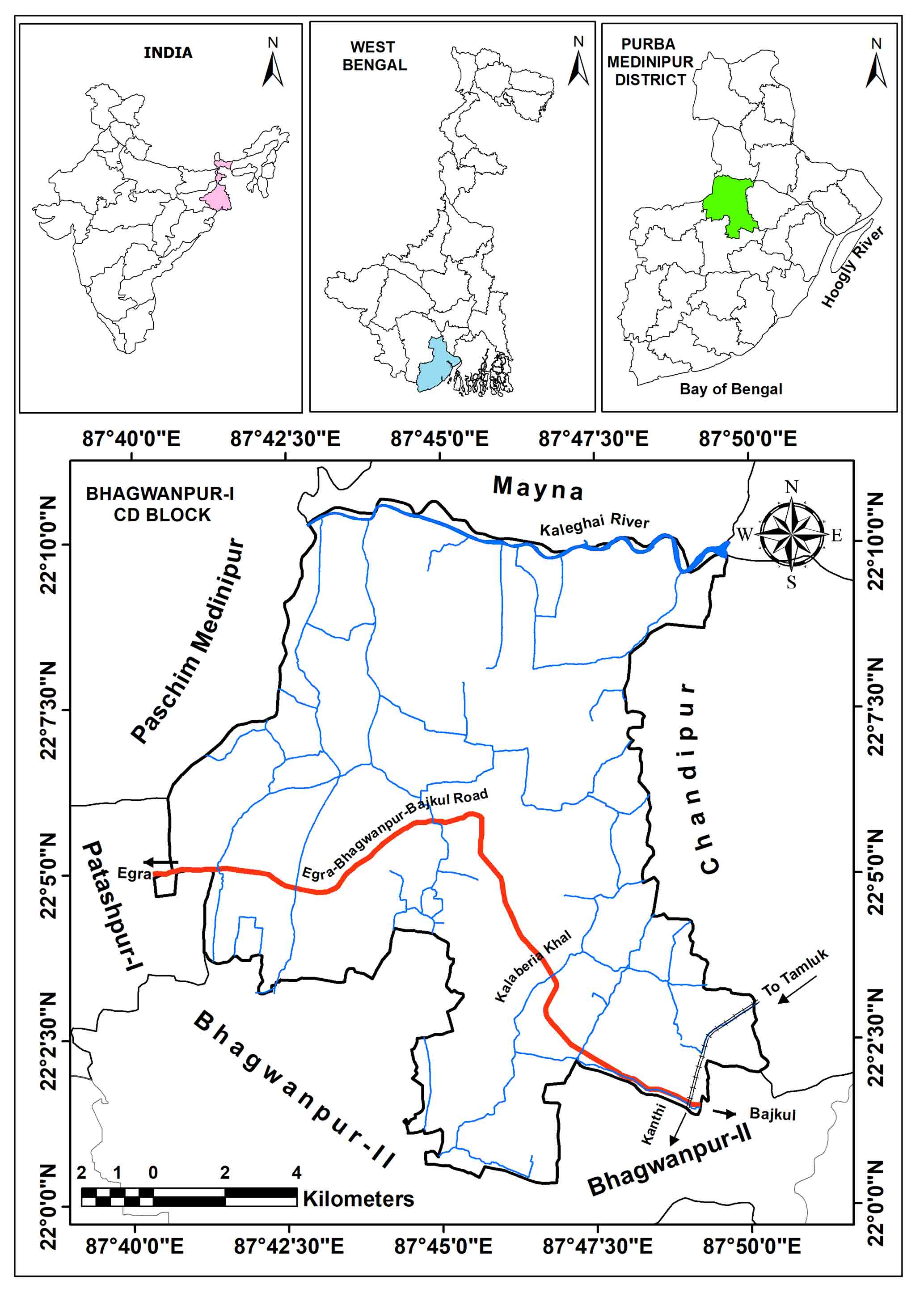
The empirical survey was conducted in the CD block of Bhagwanpur-I to collect the soil samples. The water supply intervals and 52 land parcels selected for soil sample collection, and the dimensions of land parcels were measured (Table 1). The soil samples were collected in tighter air bag since these parcels on 24^th March 2021. The corresponding latitude and longitude locations of the soil sample collection points were measured using GPS with 1m accuracy.

3.1.2 Satellite data and Pre-processing

3.1.2.1 Landsat 8 (OLI) Data

The moisture content of the agricultural field was evaluated using Landsat-8 OLI data. The Landsat 8 sensor provides multi-spectral imagery with 11 spectral bands, counting two NIR bands. The spatial resolution of OLI data is 30m, although the TIRS sensor delivers thermal imagery with a ground resolution of 100m, which was resampled to 30m. The communal method mainly used to resample the remote sensing data using a bi-linear interpolation. Using a weighted average of the neighboring pixels in the original image, bi-linear interpolation calculates the values of the each new pixel in the resampled image. The data was downloaded from web-portal (https://earthexplorer.usgs.gov/) of United States Geological Survey (USGS) recorded on 25^th April 2021. To avoid cloud contamination, images with minimal cloud cover were selected (path 138 and raw 45).

3.1.2.2 Sentinel-2B Data

In the study, Multispectral Instrument (MSI) was used to identify the permanent water body, vegetation, build up area and crop land. We can use USGS open source data portal to download the Sentinel-2A and 2B data recorded on 25^th April, 2021. Sentinel-2A and 2B are both part of the European Union Copernicus platform, and they provide multispectral imagery with high spatial resolution on chronological break of 5 days. Sentinel-2B covered the visible, NIR and SWIR regions with the 13 spectral bands, and ground coverage of 10, 20, and 60m depending on the band. As an illustration, the spatial resolution of the visible and NIR bands is 10m, whereas the spatial resolution of the SWIR bands and the four vegetation red edge bands is 60m. The spatial resolution of the coastal aerosol, water vapor, and SWIR cirrus bands is 60m.

Figure 1. Location of the study area

3.2 Pre-processing

The methods used for calculating sensor radiance for Landsat 8 satellite imagery are:

\(L=[ \{ (\frac {Lmax-Lmin}{QCalmax-QCalmin}) \times (QCal-Qcalmin) \}+Lmin]\)     (1)

where, the radiance value is maximum spectral radiance Lmax, Lmin is the minimum spectral radiance, maximum calibrated quantization level is QCalmax and QCalmin is short for qualified quantization.

This formula takes into account the range of values for the calibration level of quantization (QCal), the minimum and maximum spectral values and a constant offset term (Lmin). The spectral radiance values are affected by atmospheric correction and required to remove these effects and obtain accurate reflectance values and land surface temperature (LST) measurements. The radiance values obtained from equation (1), were used for atmospheric alteration to determine the Red, NIR, and SWIR band reflectance values, in addition for scheming the LST or Land Surface Temperature values to the thermal-infrared spectral band of Landsat 8 (OLI) data. The Level-1C products generated from sentinel-2B data are pre-processed and come using the values of top-of-atmosphere reflectance, and atmospheric correction was performed consuming the SNAP device in the sentinel application platform. NDVI, which was predicted by Rouse et al. (1974) is a commonly used to measure the vegetation intensity and red and NIR bands to use for calculating spectral reflectance.

NDVI= (NIR-RED)/ (NIR+RED)              (2)

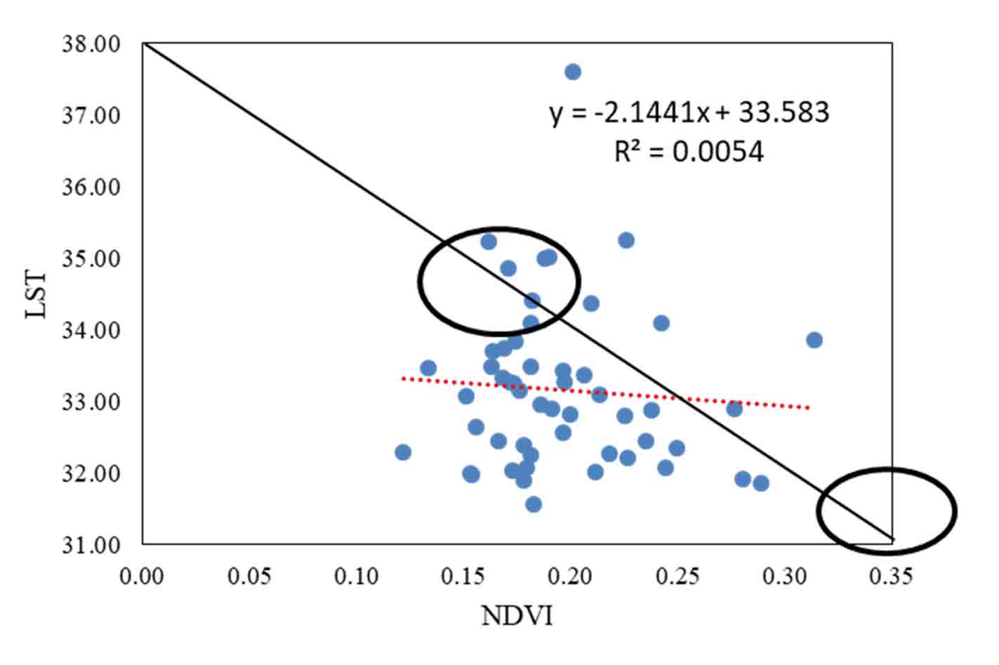
where, NDVI has been widely used for analysis of vegetation intensity and based on the association with the spectral reflectance values of NIR and Red bands. While it able to deliver information of plants healthiness and density, it is not directly related to soil moisture content. Therefore, combining NDVI and LST data can help differentiate between areas with similar vegetation cover but different soil moisture conditions. The scatter plot of LST and NDVI values can make known the soil-vegetation patterns and the distribution of the scatter plot can help extract the Soil Dryness Index Composite (SDIC) that performed for the evaluation of moisture content on the earth surface.

3.3 Top-of-Atmosphere’s Spectral Radiance

The DN values captured by the satellite sensors need to be converted to TOA radiance values for further analysis. This conversion is done using algorithms provided by the USGS website of the Landsat 8 missions. The conversion algorithm takes into account the calibration coefficients provided by the satellite manufacturers and the radiance of the sun at the moment of acquisition. The values responsible for TOA radiance are then used for atmospheric correction and other analysis. The radiometric correction was completed in the Landsat 8 (OLI) bands using the equation (3) in Arc GIS.

\(Lλ = M×P+A\)            (3)

where, Lλ= Spectral radiance (w/cm2μm), M is radiance multiplication scaling factors, A is radiance additive scaling factor for the spectral band, P is pixel values.

The equation (3) is performed to determine the Normalized Difference Vegetation Index (NDVI) for images captured by the satellites Landsat 8(OLI) and Sentinel 2B, for Landsat 8 (OLI), the spectral bands 5 and 4 stand for the NIR and Red bands, respectively, while for Sentinel 2B, the spectral bands 4 and 3 represent the equivalent. Brightness Temperature (kelvin) (equation (4)) was derived for the Land Surface Temperature (LST) from the Landsat 8 imagery.

\(T_B= \frac {K^2}{in(k^{1/2}+1)}\)              (4)

where, T_B is brightness temperature, L = Radiance is obtained from (equation (1)), K¹ and K² = Calibrated constant values get to the image metadata, K¹ and K² constant of band 10 is 774.8853 and 1321.0789, respectively. The function of LST of any region depends on the thermal emissivity for the vegetation function is:

\(P_V= (\frac {NDVI-NDVImin}{NDVImax-NDVImin})^2\)         (5)

where, Pv stands for the vegetation functions, and NDVImax and NDVImin are the minimum and maximum NDVI values. Sobrino et al. (2004) used the Pv values to get the value of emissivity (E).

\(E=0.004×Pv+0.986\)      (6)

The finally, LST was calculated using (equation (7)).

\(LST= \frac {T_B} {1+{\frac {(0.00115*T_B )} {1.4388}\times In(E)}}\)        (7)

It is not possible to establish a directly association among the NDVI and LST for Sentinel-2B imagery since it does not have a thermal band. However, if the assumption is made that the NDVI and LST acquired from Landsat 8 (OLI) data of the similar region and time period have a direct relationship, then it may be possible to use this relationship to estimate LST values for the Sentinel-2A NDVI data. This is constructed on the statement that the vegetation conditions for the two datasets are similar. It is important to note that this approach may have some limitations and uncertainties due to differences in the spatial and spectral resolution, atmospheric conditions and other factors that can affect the relationship between NDVI and LST.

3.4 DEM Data: Per-processing

DEM data, we can use some GPS survey in the region to collect the elevation data and generate it in the DEM with latitude, longitude in particular away. Than IDW in all data set and generate a DEM for SSM estimation. The North to South cross section line has a total length of 16.09km, with a maximum slope ranging from 1°45'18" to 1°50'42". The average slope of this cross section line is 0°24'18" and the minimum elevation value is 0.914m, while the maximum elevation value is 9.7536m. On the other hand, the West to East cross section line has a total length of 12.15km, with a maximum slope ranging from 1°53'24" to 1°56'6". The average slope of this cross section line ranges from 0°24'18" to 0°27'0". The minimum elevation value of this cross section line is 2.45m, while the maximum elevation value is 8.53m (GPS survey, Google Earth image and Alos Palser DEM).

3.5 Field Survey with Validation

As geospatial technology-based product is the foundation of natural resource management and decision-making process, it is very much useful for mitigating the error and accuracy assessment by using some algorithm. Accuracy is considered to truthiness of the result. GPS base survey validates the ground data to the image (Figure 2).

Figure 2. Soil Samples and GCP collection point of the study area

3.6 METHODOLOGY

3.6.1 Field Study

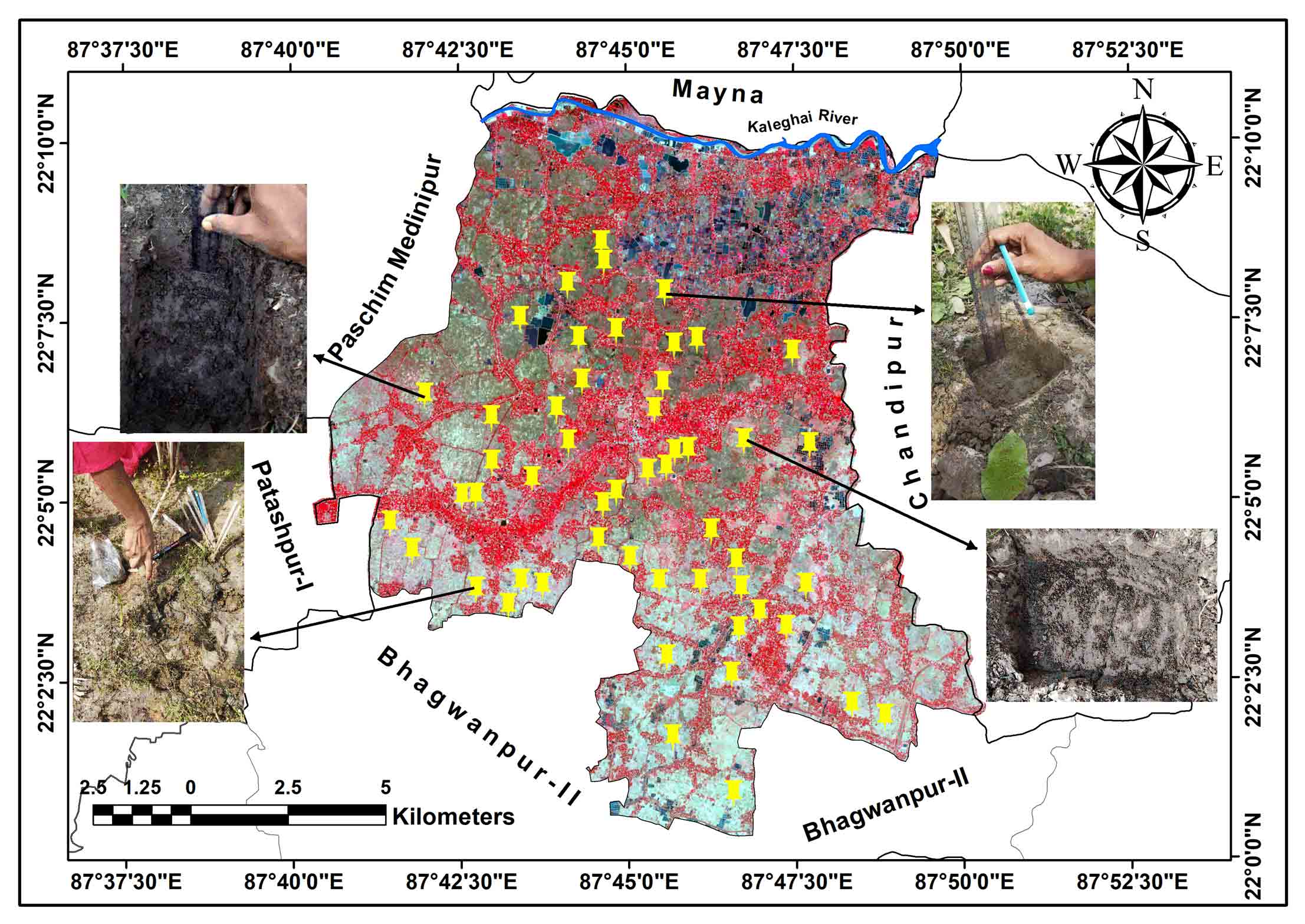
Field work was done on 25^th April 2021 to collect the major soil samples. The measuring surface soil moisture using direct from the soil samples is a reliable technique. The randomized sampling procedure is also a good approach to ensure representative soil samples. The collection of 52 soil samples at 0-10cm depth, through a width of 110cm and length is 18cm is sufficient to obtain a good spatial distribution of soil moisture data (Figure-8). Geo-referencing the sampling points using a handheld GPS system is also important to accurately locate the sampling points in the study area. It is also good to hear that the soil samples were reassigned to a soil laboratory for further analysis of surface soil moisture.

3.6.2 Gravimetric Methods uses for Surface Soil Moisture

The gravimetric method is a conventional technique for measuring soil moisture content. This method, a recognised weight of the soil samples is taken and then dried in a shiver machine at a quantified temperature for a stated period of time till all the water has been disappeared from the soil. The dry weight of the soil is then measured and by subtracting the dry weight of the original soil mass and dividing the result by the dry weight, the moisture content of the soil is taken into explanation (Younis and Iqbal, 2015). In the study area, soil samples were taken using a gravimetric technique at a depth of 1 to 5cm. After collection, the soil samples were transformed to a soil laboratory and all samples were dried in an oven at a temperature range of 85℃-110℃ for 30 minutes. The soil moisture content was calculated using the gravimetric method, which provides a perfect measurement of content of soil moisture at a specific depth. These measurements can be used to validate and calibrate remotely sense used for mapping the surface soil moisture. This method involves collecting the soil samples from the fields, drying them in an oven and measuring sample weight before and after drying to calculate the soil moisture content. The distribution of our test location of surface soil moisture is mostly affected by irrigation and rainfall patterns. Therefore, it is important to collect soil samples simultaneously with the satellite image acquisition to ensure that the data accurately indicates the moisture levels in the soil top layer. By averaging the gravimetric reading from various soil samples taken from the test location, the average values of the surface soil moisture content may be intended.

\(Gravimetric \ Soil \ Moisture \ (Sg) = \frac {Ws-Wd}{Wd} \times100\)   (8)

\(Builk \ Density \ (Pb) \ = \frac {Ws}V\)           (9)   

\(Valumetric \ Soil \ Moisture \ (Sv)\ = Sg \times Pb \)      (10) 

where,  is weight of soil moisture,  is weight of dry soil samples is volumes of soil samples. The Gravimetric Soil Moisture ( ) values were calculated for each test site.

Figure 2. Soil Samples and GCP collection point of the study area

3.6.3 Estimation of Soil Moisture through the Remote Sensing data

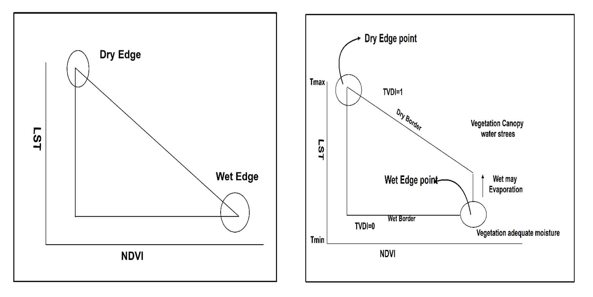
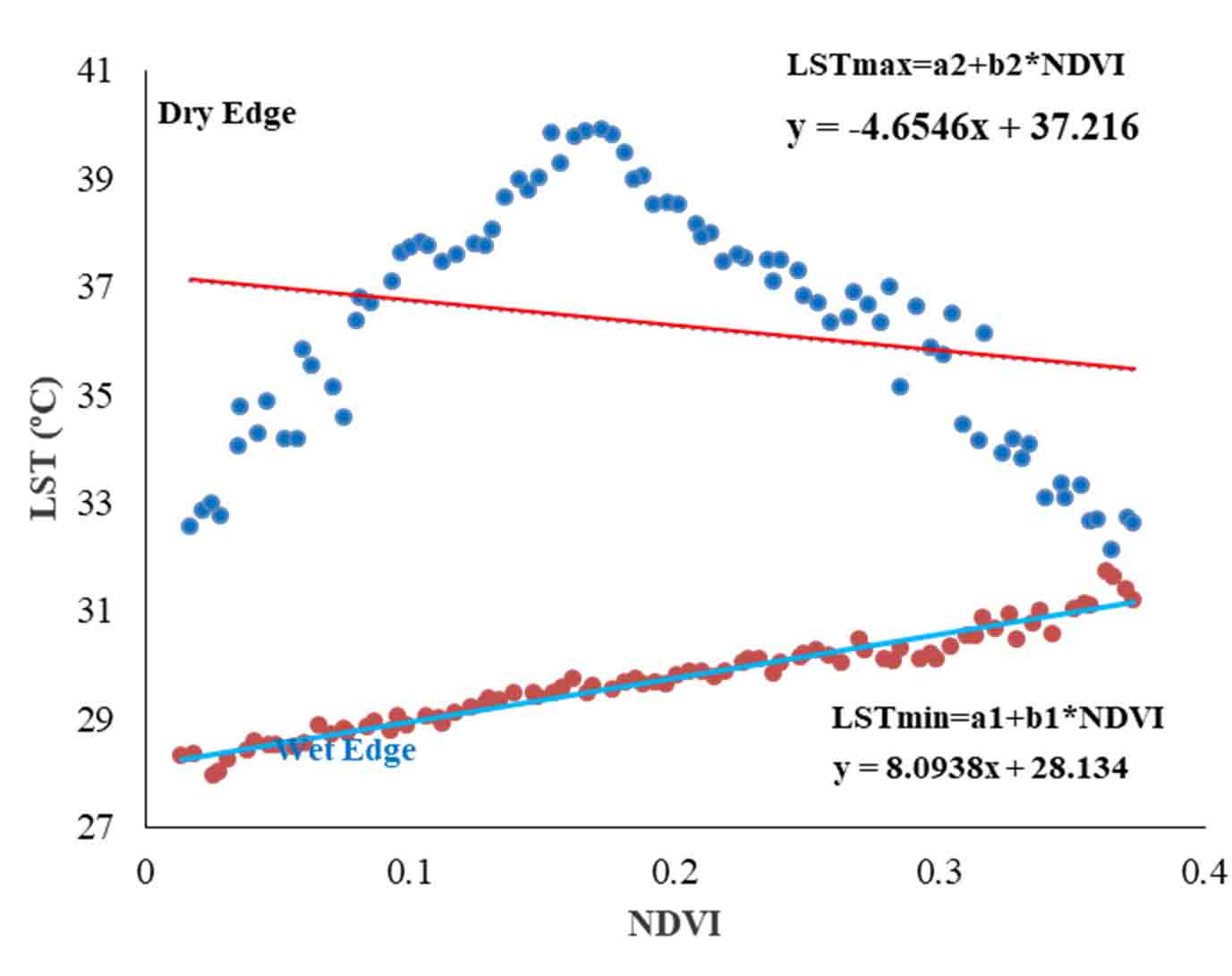
Temperature Vegetation Dryness Index (TVDI) is a method that uses Landsat-8 imagery to assess the surface soil moisture content through the combining optical datasets such as: visible, infrared and thermal bands. NDVI and LST utilize plants and water stress and the foundation of the TVDI techniques. The link between thermal and visible/NIR data is used in the TVDI method to map soil moisture. The distribution of pixels values in Ts-NDVI space is interpreted to identify a huge space of the soil water content and the triangle-shaped greenery that surrounds it. This triangle is designed since, decreased surface temperature as increased vegetation cover. By combining LST-NDVI space and TVDI approaches, which have a tight relationship to surface temperature and surface soil moisture into a scatter plot.

3.6.4 Theatrical Background NDVI and LST Spectral Space for Estimation of Soil Moisture

The pixel values dropping Lower Left Corner (LLC) points were places low NDVI and LST stand made patches of moist and exposed soil. The amount of pixels that were identified in the Upper left Corner (ULC) as dry, bare soil regions had high LST and low NDVI. The pixels with low LST and high NDVI in the Lower Right Corner (LRC) originate from areas of think vegetation with low soil moisture content. Therefore, distinguishing the wet and dry edges from the NDVI and LST spectral space is important from a scientific stand point since these edges are crucial for determining the minimum and maximum LST inconsistency for specific NDVI values as shown in figure (3).

Figure 3. Theoretical background of soil moisture, LST and NDVI

Figure 4. Methodology

3.6.5 Computation of TVDI

The slope (b) and intercept (a) of the dry edge and wet edge of the surface were used to determine the LSTmax and LSTmin, two important edge numbers. Equation 14a and 14b. The LST of dry and wet soil is what LSTmax and LSTmin are made up. The subsequent equation was performed to determine the maximum and minimum LST for the dry edge and wet edge of the surface.

\(LSTmax=a1+b1×NDVI\)  (11a)

\(LSTmin=a2+b2×NDVI\)  (11b)

where, NDVI stands for the Normalized Difference Vegetation Index, the intercepts of the dry and wet edges are (a1) and (a2), respectively, and the slopes of the dry and wet edges are (b1) and (b2), respectively. So it can determine dry and wet values from the TVDI image. The minimum and maximum LST values can use for calculating surface soil moisture content of the equation (12).

TVDI= ((LST-LSTmin)/ (LSTmax-LSTmin)) (12)

where, TVDI is Temperate Vegetation Dryness Index, and LST values are obtained from the Landsat 8 (OLI) imagery.

4 . RESULTS AND DISCUSSION

The foremost aim of the study was to use optical multispectral images to assess the soil moisture status in the upper layer of the agricultural area in Bhagwanpur-I CD block. The finding demonstrates that it is possible to estimate the surface soil moisture content using satellite images from Landsat 8 (OLI) and sentinel 2B. The visible, NIR and thermal infrared dataset were used in the triangulation method for developed the created TVDI map with the LST and NDVI. The study found that gravimetric methods provide more precise soil moisture data compared to indirect measurement methods. The minimum and maximum LST values of wet and dry soil are used to calculate the wet edge and dry edge in the LST-NDVI spectral space.

4.1 Soil Moisture Estimations using Optical Satellite Data

TVDI method is established in the observations that surface temperature fell as vegetation cover increased. A connection between surface energy and moisture status was built using data from LST and NDVI measurements. From the TVDI image, a vast area of vegetation and soil moisture content was extracted, generating a triangle in the Ts-NDVI space. For estimating the minimum and maximum LST predictability at specific NDVI values, the Ts-NDVI triangle space with dry edge and wet edge of the surface was used. These maximum and minimum LST values are provided to evaluate the surface moisture in the upper layer of agricultural areas in the Bhagwanpur-I block of East Medinipur, West Bengal.

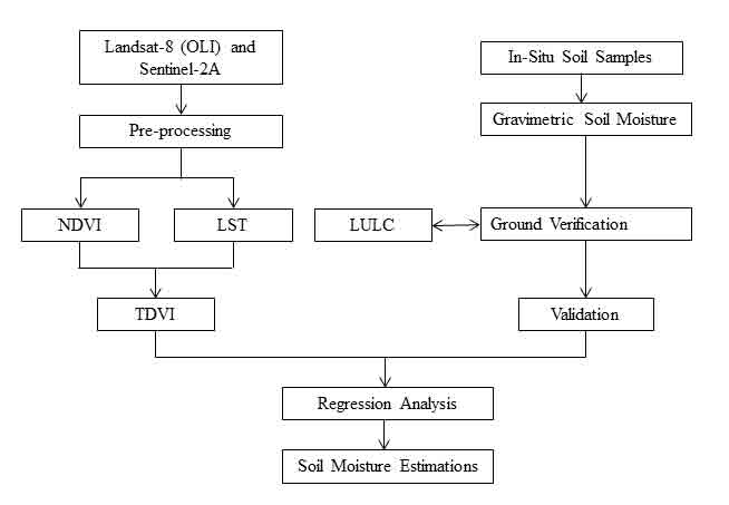
4.1.1 NDVI

NDVI is calculated using the reflectance patterns of vegetation leaves in the visible and near-infrared spectra. Because of the visible region (0.4-0.7 micrometers) is largely absorbed by the healthy chlorophyll concentration in vegetation. The NDVI values range between -1 and +1, where values close to +1 and 0 that’s specify dense green vegetation and bare soil or rock respectively, another, the values close to the -1 indicate water. In the study, the NDVI values ranged from 0.02 to 0.54. A study and statistical evaluation of the NDVI-LST model’s accuracy in estimating soil water content was conducted. The results showed that the ability of model to estimate the soil moisture was enhanced by substituting NDVI for EVI. The arrangement of the study space into five major NDVI classes based on vegetation intensity is a valuable tool for considerate the distribution of vegetation and its relationship with soil moisture content (Figure 5). The highest vegetation intensity was found in the middle and southeastern parts of the study area (57.38km²; 31.37%) (Table 1). In contrast, the areas with very low and low vegetation intensity is 7.32km² and 34.34km² (4.00% and 18.78%), respectively mainly located in the northern part where soil moisture content is high. Moderate and very high vegetation intensity estimated for the area about 55.25km² and 28.63km² (30.19% and 15.65%), respectively (Table 1). The findings imply that the spread of vegetation in the studied region is significantly influenced by the soil moisture content.

 

Table 1. Distribution of NDVI

Classes	Values	Area
		km2	%
Very low	-0.16683	07.31	4.00
Low	0.09564 - 0.1709	34.34	18.78
Moderate	0.17100 - 0.2157	55.22	30.20
High	0.2158 - 0.2645	57.38	31.37
Very high	0.2646 - 0.4476	28.63	15.65
Total		182.88	100

 

Figure 5. NDVI

 

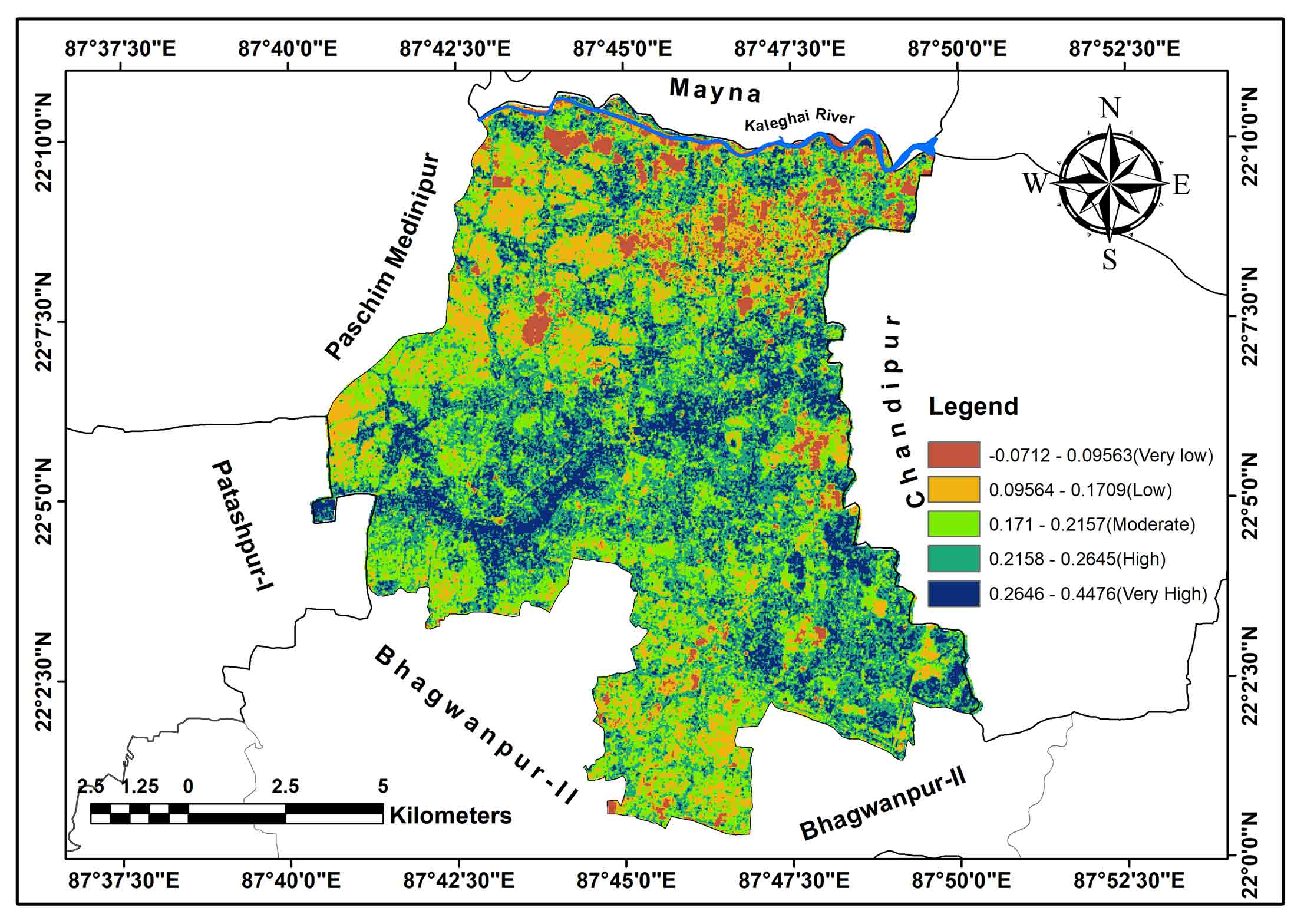
4.1.2 LST

The relationship between the LST and processes including evapotranspiration, surface energy balance, and vegetation development makes it a crucial in environmental studies. TIR of a Landsat-8 satellite image was used to compute LST. To estimate the LST, the average values of the two bands: TIR 10 and 11 bands were used. Two procedures were taken in order to translate the thermal digital numbers (DN) into actual surface temperature measurements. The top of the atmosphere (ToA) radiance was firstly converted into the ToA brightness temperature in Kelvin and then back to the ToA radiance values. Using the formula c=k-273.15, the temperature data were finally converted to degrees Celsius. The TIR bands and surface emissivity can be used to estimate LST and surface emissivity, respectively. If both LST and surface emissivity are needed, Landsat-8 (OLI) data can be combined with other satellite data, such as MODIS data, to obtain a higher temporal resolution. However, atmospheric correction is required to remove the effects of atmospheric water vapor, aerosols and clouds that can affect TIR radiation. The obtained LST values ranged from 28.25ºC to 39.09ºC. The temperature map (Figure 6), which depicts the temperature variation among the research locations, was produced using the Arc GIS environment. The study area appears to have been divided into five main groups based on LST. The largest area was covered by the moderate temperature class, which accounted for 44.45% (80.77km²) (Figure 6). The other classifications, which comprised 5.18% (9.43km²), 29.36% (53.35km²), 7.75% (14.10km²) and 13.27% (24.17km²), respectively were very low, low, high, and very high (Table 2). The middle and southern portions show very little water in the soil. On the other hand, the northern region shows water bodies predominantly and soil water content is very high.

 

Table 2. Distribution of LST

Classes	Values	Area
		(km2)	(%)
Very low	28.22 - 31.29	9.43	5.19
Low	31.3 - 32.57	53.38	29.36
Moderate	32.58 - 33.59	80.77	44.43
High	33.6 - 35.04	14.10	7.76
Very high	35.05 - 39.09	24.12	13.27
Total		181.80	100

 

Figure 6. LST

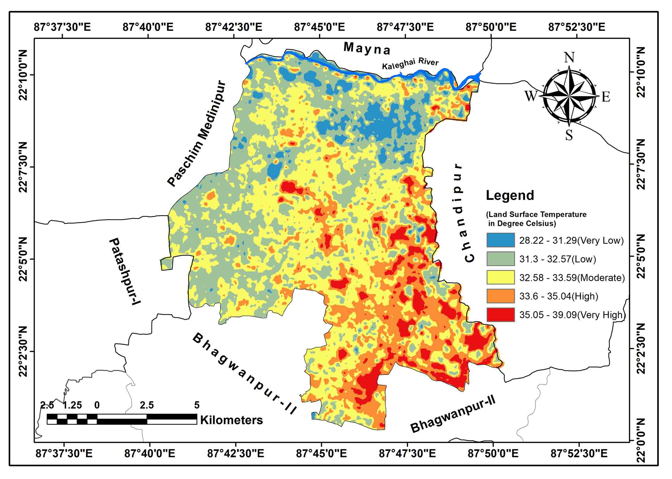
4.1.3 TVDI

TVDI is computed using the determined values of LST and NDVI. TVDI is a variant of the Vegetation Drought Index (VDI) that takes into account the temperature and vegetation components separately. The LST and NDVI readings were plotted against one another in Excel sheets to form the Ts-NDVI space. In order to identify the wet-dry edge of the surface in the research area, regression lines were created to define the upper-lower edge of the triangle. This method helped for image classification of the wet-dry edge based on the distribution of LST and NDVI pixels. An analysis of the triangle formed by the distribution plot of LST and NDVI representative the Ts-NDVI planetary data. Sandholt et al. (2002) used this area for the classification of TVDI. It was considered by subtracting the minimum potential evapotranspiration (PET) from the actual evapotranspiration (ET), which was estimated using the LST and NDVI values. The TVDI values vary from -1 to 1, with destructive values representative wet environments and constructive values representative of dry environments.                

There is a strong association among LST and NDVI, with LST declining as NDVI increases during the growing season. This relationship can be used to detect the slope of the NDVI-LST curve, which can be successfully determined throughout the growing season. This information can be useful for estimating in-situ soil moisture, as the NDVI incline from image windows remained found to be meaningfully associated with the surveyed soil moisture (Xin et al., 2006). This relationship between LST and NDVI is important in the calculation of TVDI. The TVDI is calculated the LST and NDVI values, as the minimum and highest LST values. The values of TVDI range from 0 to 1 with higher values are signifying drier environment (Figure 7). Five classifications can be seen on the TVDI map: low, moderate, high, and very high. The very low and low TVDI values cover 15.45% (28.21km²) and 34.82% (63.58km²), respectively. This area is mostly found in the northern-eastern part of the study area where more water content in the soil. The moderate TVDI values are observed on the area about 29.45% (53.78km²) especially in the southern and middle regions with moderate soil moisture. The high and very high TVDI values estimated about 14.67% (26.79 km²) and 5.61% (10.25 km²) study area, respectively.

Figure 7. TVDI

4.2 Relationship and spatial variation of the NDVI-LST

Significant spatial variation in LST and NDVI shows favourable in south-eastern part and less positive correlation is observed in the south-western part (Figure 8).

 

Figure 8. Distribution of LST and NDVI

 

Figure 9. Dry edge and wet edge of the land and water surfaces are defined by the NDVI-Ts space

4.2.1 The Validation of GSM and Remote Sensing Derived Soil Moisture

It is stimulating that there is the less positive relationship among the TVDI and actual soil moisture content to the Rout Mean Square Errors (RMSE) was documented as 0.175. The TVDI, which was based on a combination of surface temperature and NDVI, was found to be more accurate in regional drought assessment. To conclude the TVDI and dryness index are effective in apprehending the spatial disparity of the condition of soil moisture for illustration of soil moisture (Figure 14).

A SSM map with the classifications of extremely low, low, moderate, high, and very high was created based on the TVDI map. The very low and low SSM values observed for 6.00% (10.97km²) and 14.19% (25.92km²) area, respectively typically located in the southern portion. The central and southern portions, where the soil had moderate water content with moderate SSM values. The high and very high SSM values estimated for 35.39% (64.63km²) and 15.82% (28.89km²) area, respectively show more water in the soil.

 

Table 4. RMSE between experimental soil moisture and remotely observed soil moisture

Sample Points	Gravimetric Soil Moisture	TVDI	Residual	Square of Residual	RMSE
S1	0.0638	0.7777	0.2825	0.0798	0.174933
S2	0.1765	0.6236	0.0910	0.00827
S3	0.1786	0.6604	0.1271	0.01615
S4	0.2658	0.4484	-0.1139	0.01296
S5	0.2346	0.3617	-0.1902	0.03617
S6	0.0638	0.3688	-0.1264	0.01598
S7	0.1549	0.7069	0.1815	0.03294
S8	0.2025	0.8475	0.3062	0.09378
S9	0.0337	0.425	-0.0602	0.00362
S10	0.0482	0.537	0.0470	0.00221
S11	0.0877	0.4835	-0.0196	0.00038
S12	0.0976	0.5492	0.0428	0.00183
S13	0.1628	0.5044	-0.0237	0.00056
S14	0.2048	0.2729	-0.2691	0.07244
S15	0.2206	0.2656	-0.2816	0.07932
S16	0.1447	0.6096	0.0875	0.00766
S17	0.1765	0.4255	-0.1071	0.01146
S18	0.1507	0.517	-0.007	0.00005
S19	0.1837	0.6036	0.0686	0.00471
S20	0.1429	0.7062	0.1847	0.03412
S21	0.1647	0.4892	-0.0395	0.00156
S22	0.1228	0.3459	-0.1689	0.02853
S23	0.1159	0.3562	-0.1563	0.02442
S24	0.0964	0.2758	-0.2302	0.05297
S25	0.1364	0.328	-0.1913	0.03658
S26	0.1236	0.3364	-0.1787	0.03192
S27	0.1628	0.5507	0.0226	0.00051
S28	0.1236	0.4673	-0.0478	0.00228
S29	0.1628	0.7996	0.2716	0.07374
S30	0.1905	1.1967	0.6594	0.43483
S31	0.2727	0.6239	0.0593	0.00352
S32	0.1625	0.5402	0.0123	0.00015
S33	0.1364	0.571	0.0517	0.00268
S34	0.1731	0.5597	0.0282	0.0008
S35	0.1892	0.4699	-0.0669	0.00448
S36	0.1628	0.3814	-0.1467	0.02152
S37	0.1286	0.5736	0.0569	0.00324
S38	0.1600	0.3571	-0.1700	0.0289
S39	0.1294	0.5235	0.0065	0.00004
S40	0.1235	0.6662	0.1512	0.02286
S41	0.1071	0.8264	0.3168	0.10035
S42	0.0204	0.3504	-0.1304	0.017
S43	0.0526	0.3746	-0.1169	0.01366
S44	0.1587	0.3384	-0.1884	0.03548
S45	0.0638	0.8041	0.3089	0.09543
S46	0.1111	0.4553	-0.0556	0.0031
S47	0.0233	0.3953	-0.0864	0.00746
S48	0.1628	0.4224	-0.1056	0.01116
S49	0.0753	0.4563	-0.0427	0.00182
S50	0.1765	0.5379	0.0053	0.00003
S51	0.1111	0.5712	0.0603	0.00364
S52	0.1494	0.4133	-0.1103	0.01217

 

Figure 10. Soil moisture estimated using remotely sensed data

Table 5. Area of soil moisture derived from multi-spectral data

Classes	Values	Area
		km2	%
Very low	0.1-0.16677	10.97	6.01
Low	0.1678-0.3766	25.96	14.19
Moderate	0.3767-0.5234	52.21	28.59
High	0.5235-0.6645	64.63	35.39
Very high	0.6646-1.071	28.89	15.82
Total		182.62	100

 

 

4.2.2 Validation of Soil Moisture Measurements Obtained Using Remote Sensing

A critical step in guaranteeing the correctness and dependability of the acquired data is the validation of LULC derived from satellite imagery. The validation process involves comparing the satellite image with ground truth information to assess the level of agreement or disagreement. The following are some typical techniques for validating LULC generated from remote sensing: Crowdsourcing, statistical analysis, expert assessment, visual interpretation and gathering real-world data. A combination of the above methods can be used to validate the data, depending on the project requirements and available resources. The LULC map use in this project is generated from Sentinel-2A image using unsupervised classification. This LULC image is classified into 5 categories as: water bodies, vegetation, fallow land, settlements and agricultural lands. The maximum area agricultural lands and vegetation are covered by 44.8907 % (15.4817km²) and 1.141228% (69.6432 km²), respectively they are mostly located in in the middle and northern parts as well as the southern to western parts in the study. The lowest water bodies, fallow lands and settlements are covered 8.494303% (15.4817 km²), 1.141228% (2.08 km²) and 7.262819 % (13.2372 km²) area, respectively (Figure 11 and Table 6).

Figure 11. LULC

Table 6. Distribution of LULC

Classes	Area
	km2	%
Water bodies	15.48	8.49
Vegetation	69.64	38.21
Fallow land	2.08	1.14
Settlements	13.24	7.26
Agricultural lands	81.82	44.89
Total	182.26	100

 

 

4.2.3 Gravimetric Soil Moisture

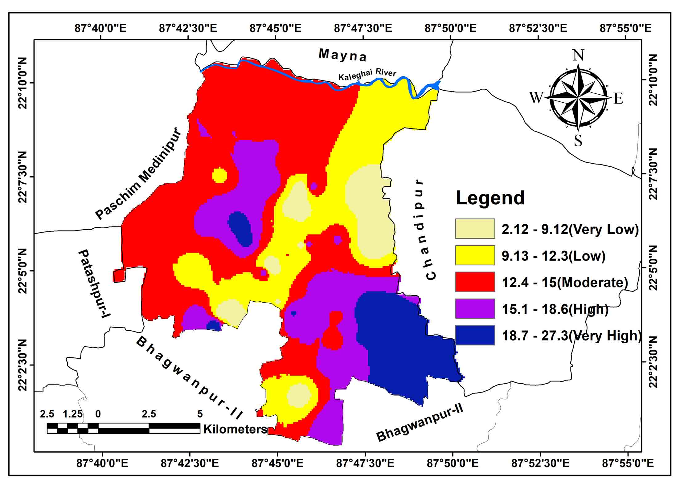
Maps showing GSM and SSM based on TVDI provide information on soil moisture they are based on different methods of measurement and therefore can have differences the values of soil moisture distribution in space. It is wealth observing that the GSM map were based on direct in-situ soil samples, it provide more accurate measurements of the soil moisture in the locations where soil samples were taken, but may not always accurately reflect the soil moisture levels across the research area. However, due to factors including cloud cover and soil type, the precision of the TVDI-based SSM map, which offers a more thorough assessment of soil moisture conditions across a greater area, may be questionable. In order to comprehend the soil moisture in the research region more completely, it is crucial to take into account both maps (Figure 12; Table 7).

 

Table 7. Gravimetric soil moisture

Classes	Gravimetric Soil Moisture (%)	Area
		km2	%
Very low	2.12-9.12	14.12	7.75
Low	9.13-12.30	38.77	21.26
Moderate	12.40-15.00	77.58	42.55
High	15.10-18.60	31.80	17.44
Very high	18.70-27.30	20.06	11.00
Total		182.35	100

 

 

Figure 12. Gravimetric soil moisture

 

4.2.4 Soil moisture based on models

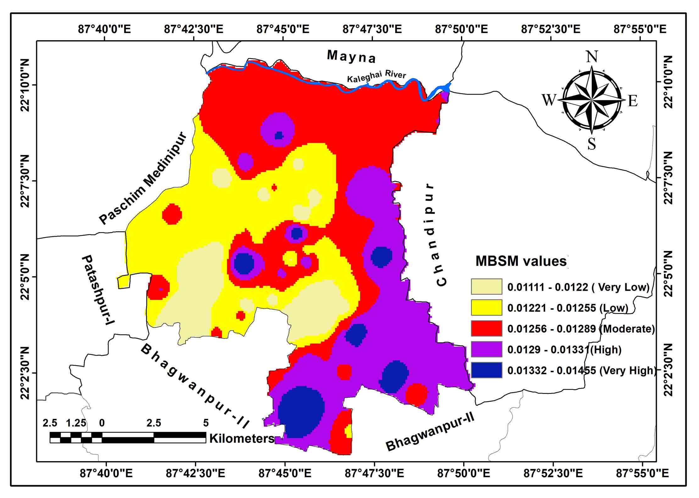
The Model Based Soil Moisture (MBSM) Map was created by comparing in-situ soil moisture and backscattering coefficients. Very low, low, moderate, high, and very high were the resulting categories in the map. According to the map, 11.922% (21.736km²) of the study area has very low MBSM values and 24.183% (44.089km²) has low MBSM values. These values are primarily found in the study area’s central and western regions, where there is less water in the soil. The third type, moderate MBSM values, covers 31.857% (58.078km²) area and is found of northern and some middle part in the study area where the soil has a moderate amount of water. Lastly, the high and very high MBSM values cover 27.813% (50.706km²) and 4.224% (7.700km²), respectively located in the south and southeast portion in the study area where very high water content in the soil observed (Figure 13; Table 8).

Table 8. Model based soil moisture

Classes	MBSM Values	Area
		km2	%
Very low	0.01111-0.0122	21.74	11.92
Low	0.01221-0.01255	44.09	24.18
Moderate	0.011256-0.01289	58.08	31.86
High	0.0129-0.0133	50.71	27.81
Very high	0.01332-0.01455	7.70	4.22
Total		182.31	100

 

 

Figure 13. Model Based Soil Moisture

 

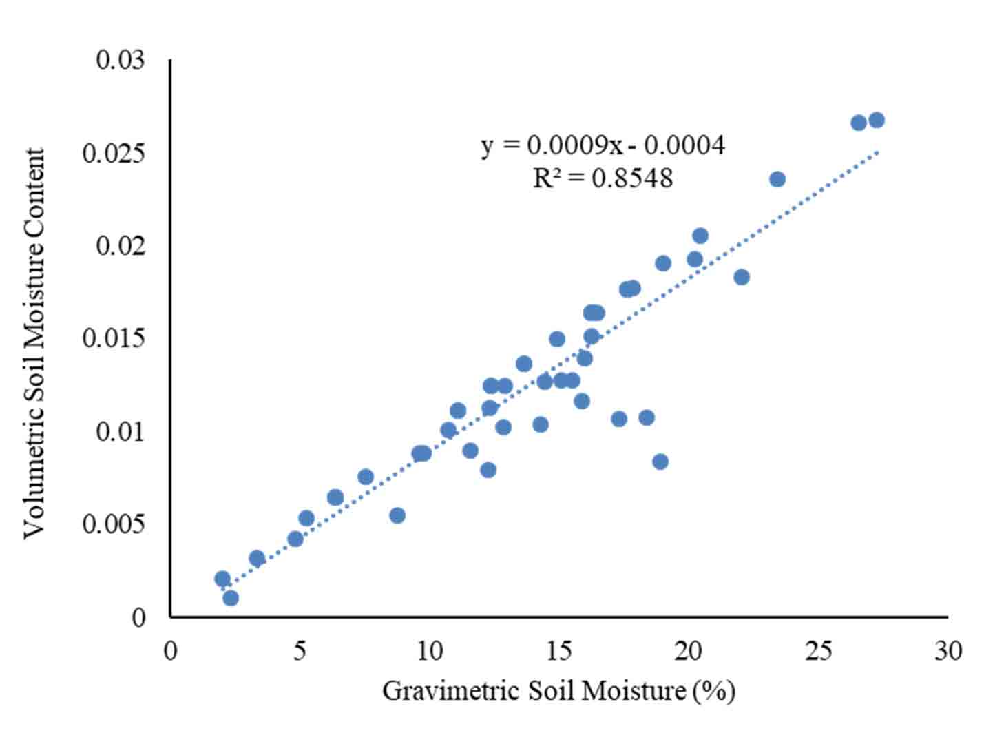
4.2.5 Relationship between Volumetric Soil Moisture and Gravimetric Soil Moisture

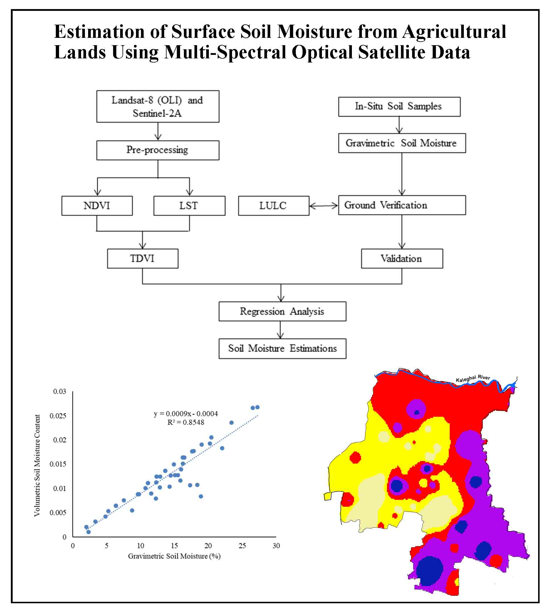
Two approaches are frequently used to gauge how much water is present in soil are: 1) moisture content measured by gravity and 2) soil moisture measured by volume. Volumetric soil moisture content is expressed as a percentage of the total soil volume, but gravimetric soil moisture is frequently expressed as a percentage of the dry weight of the soil. The relationship between these two measures of soil moisture can be complex and is influenced by a number of factors, including soil texture, porosity and organic matter content. In the study, gravimetric soil moisture and volumetric soil moisture content have a strong positive connection (R²= 0.8548), with greater gravimetric soil moisture values often suggesting higher volumetric soil moisture content. This correlation can be quantified using various arithmetic procedures, which can be performed to control the nature, intensity, and direction of the link among the two variables (Figure 14; Table 9). However, it is crucial to keep in mind that the precise relationship between gravimetric soil moisture and volumetric soil moisture content might change based on the exact kind of soil and environmental factors in a given study region.

 

Figure 14. Gravimetric soil moisture and volumetric soil moisture

 

Table 9. Gravimetric soil moisture content and volumetric soil moisture content

Samples	Latitude	Longitude	Gravimetric soil moisture (%)	Volumetric soil moisture content
S1	22.02794	87.76105	6.38298	0.0064
S2	22.06251	87.7123	17.6471	0.0176
S3	22.01494	87.77608	17.8571	0.0177
S4	22.0325	87.81374	26.5823	0.0266
S5	22.05863	87.72033	23.4568	0.0235
S6	22.06425	87.72346	6.38298	0.0064
S7	22.09656	87.77899	15.493	0.0127
S8	22.03529	87.8056	20.2532	0.0192
S9	22.09557	87.79541	3.37079	0.0031
S10	22.0633	87.72878	4.81928	0.0042
S11	22.0693	87.75054	8.77193	0.0054
S12	22.07376	87.74275	9.7561	0.0088
S13	22.08187	87.74395	16.2791	0.0163
S14	22.09651	87.73545	20.4819	0.0205
S15	22.10418	87.73248	22.0588	0.0183
S16	22.13114	87.75949	14.4737	0.0126
S17	22.13816	87.74437	17.6471	0.0176
S18	22.12044	87.73806	15.0685	0.0127
S19	22.12225	87.74745	18.3673	0.0107
S20	22.08798	87.72629	14.2857	0.0103
S21	22.10221	87.71631	16.4706	0.0163
S22	22.09183	87.71631	12.2807	0.0079
S23	22.08409	87.70897	11.5942	0.0089
S24	22.08426	87.71227	9.63855	0.0088
S25	22.07785	87.69099	13.6364	0.0136
S26	22.07147	87.69643	12.3596	0.0124
S27	22.04246	87.77573	16.2791	0.0163
S28	22.05298	87.7776	12.3596	0.0124
S29	22.05681	87.78276	16.2791	0.0163
S30	22.05322	87.78936	19.0476	0.019
S31	22.06293	87.79429	27.2727	0.0267
S32	22.06869	87.77699	16.2500	0.0151
S33	22.0624	87.77819	13.6364	0.0136
S34	22.06396	87.76801	17.3077	0.0106
S35	22.06404	87.75783	18.9189	0.0083
S36	22.11053	87.73881	16.2791	0.0163
S37	22.14264	87.74379	12.8571	0.0102
S38	22.13301	87.73532	16.000	0.0139
S39	22.10751	87.69966	12.9412	0.0124
S40	22.08963	87.75508	12.3457	0.0112
S41	22.10389	87.75682	10.7143	0.01
S42	22.10994	87.75892	2.04082	0.002
S43	22.11878	87.76181	5.26316	0.0053
S44	22.12009	87.76747	15.873	0.0116
S45	22.11697	87.79117	6.38298	0.0064
S46	22.12513	87.72353	11.1111	0.0111
S47	22.08474	87.74718	2.32558	0.001
S48	22.0946	87.76518	16.2791	0.0163
S49	22.09409	87.7618	7.52688	0.0075
S50	22.07573	87.77077	17.6471	0.0176
S51	22.09057	87.75966	11.1111	0.0111
S52	22.04653	87.75964	14.9425	0.0149

 

5 . CONCLUSION

Temperature Vegetation Dryness Index (TVDI) approach was performed to estimate the soil moisture content in the upper layer of agricultural fields using optical data from a Landsat 8 satellite picture. Traditional methods for analyzing direct in-situ methods were used to measure the surface soil moisture. An accurate assessment of soil moisture using the TVDI method was established, and a significant association between LST and NDVI was found. Through the regression study, the surface of TVDI was formed, which was formerly associated with the gravimetric soil moisture. So, the results showed a positive association, indicating that the developed models worked well in the study area. The TVDI method was found to be effective and can be used in conjunction with in-situ measurements to improve accuracy. The results have important implications for crop growing and hydrological resource management, as a precise measurement of surface soil moisture can help optimize irrigation and water use practices.

Tables

Figures

Conflict of Interest

Acknowledgements

Abbreviations

References