Keywords

Extreme values trilemma , Probability paper , Statistical choice

1 . Introduction

Statistical decision for univariate extremes is currently at a moderate stage of development. Some problems have been effectively solved, but not all of the essential ones. On the way, many problems to be solved will appear, constituting a happy hunting ground for researchers. Curiously, even, Bayesian methods have not been strongly developed for statistical extremes, except essentially for some Reliability questions.

The analysis that follows has the following steps: once it is assumed that the useful distribution is of one of the three forms ― Fréchet, Gumbel or Weibull — we will discuss statistical decision using the assumed distribution. This chapter will be devoted to quick exploration techniques, or even as a rough guide on how to assume one of the three models. The last chapter will deal with optimal analytical techniques, comparing them, as far as possible, with the quick ones.

Note that as a matter of practical convenience we will deal with statistical decision for Gumbel and Fréchet distributions for maxima and for Weibull distribution for minima, as the latter is very important in Reliability.

The statistical techniques presented, in the all but the two last chapters, deal with complete samples and an assumed distribution; the penultimate chapter will deal with statistical choice of models and the last one with some cases of incomplete information.

Clearly the Gumbel distribution for maxima with \(\mathrm{\delta \left( >0 \right) }\) known, the Fréchet distributions for maxima with \(\mathrm{\lambda }\) and \(\mathrm{\alpha \left( >0 \right) }\)  known, and the Weibull distributions for minima with \(\mathrm{\lambda }\) and \(\mathrm{\alpha \left( >0 \right) }\) known are easily reduced to the exponential distribution (only with a scale parameter) by evident transformations, and the whole technique of the exponential distribution can be transformed to these special distributions of extremes.

2 . Assumption of a model from previous knowledge

In fact, this section could also be called “assumption by tradition”. This essentially involves a variable mixture: a convenient usage of accumulated experimentation, of limiting results to be considered as being finitely capable of fitting data, as well as some intuition. The situation is completely analogous to the assumption of normal (multinormal) distribution, where the Central Limit Theorem plays an important role as does long-term accumulated experience with measurements (1), to the assumption of binomial or Bernoulli distribution for use in repeatable trials with an approximately stable probability of the event under consideration, to the assumption of Poisson

Let us suppose that we are dealing with maxima (or dually with minima) of i.i.d. samples, with the same size \(\mathrm{n}\), and underlying distribution either as behaviour of small (random) numbers or as a limit of binomial distribution (2)  to the assumption of the exponential distribution in the (first) analysis of inter-arrival times (thus implying the Poisson distribution for the associated counting process), to the assumption of geometric, inverse binomial or Pascal distributions in stopping time experiments with the event probabilities approximately stable, etc... The situation here is very similar.

Suppose that \(\mathrm{F \left( . \right) \in }\, \mathcal{D}\, \mathrm{ ( \tilde{L} ( . ) ) ,}\) that is \(\mathrm{F(.)  } \) belongs to domain of attraction of \(\mathrm{\tilde{L}(.)  } \) (Weibull, Gumbel or Fréchet distributions), i.e., there exist sequences \(\mathrm{\{ \lambda _{n}, \delta _{n};~ \delta _{n}>0 \} ~  } \)such that \(\mathrm{ F^{n} \left( \lambda _{n}+ \delta _{n}~x \right) \rightarrow \tilde{L} \left( x \right) ,  } \) the convergence being at every point of \(\mathrm{\mathbb{R}}\) by the continuity of \(\mathrm{\tilde{L}(.)}\), and the sequences not being unique, as said before.

Then as convergence is uniform, i.e.

\(\mathrm{\begin{array}{c} \mathrm{sup} \\ \mathrm{x} \end{array}| F^{n} ( \lambda _{n}+ \delta _{n}\,x ) -L \left( x \right) \vert =\begin{array}{c} \mathrm{sup} \\ \mathrm{y} \end{array} \vert F^{n} ( y ) -\tilde{L}( \frac{y- \lambda _{n}}{ \delta _{n}} ) \vert \rightarrow 0, }\)

for large \(\mathrm{n}\), we can assume that there exists \(\mathrm{\left( \lambda ,~ \delta ;~ \delta >0 \right) }\) such that \(\mathrm{F^{n} \left( y \right) \approx\tilde{L} ( \frac{y- \lambda }{ \delta } ) . }\)

Also \(\mathrm{\tilde{L}(.)}\) satisfies the stability equation \(\mathrm{\tilde{L}^{t} ( x ) =\tilde{L} \left( \alpha _{t}+ \beta _{t}~x \right) , \beta _{t}>0. }\)

The heuristic reasoning used by Fisher and Tippett (1927/28),(p.180), shows approximate stability of maxima.

Thus, with the uniformity of convergence and the (approximate) stability of maxima, we can use the approximation \(\mathrm{F^{n} \left( y \right) \approx \tilde{L} \left( \left( y- \lambda \right) / \delta \right) .~ }\)

But what happens when \(\mathrm{F(.) }\) is one of those “awkward” distributions that are not attracted to one of the \(\mathrm{\tilde{L}'s~? }\) This, in general, is a consequence of high tails (the right-tail for maxima), and the use of “slowing down” transformations as the \(\mathrm{log(.) }\) or \(\mathrm{log\,log(.) }\) can be useful; recall the example given in Part-1.

Note that the approximation to \(\mathrm{F^n(y) }\) depends on the size of the sample \(\mathrm{(n) }\); accumulated experience and simulation can give some idea when the fit is good or even reasonable.

It should be noted that in the heuristics given before we assumed i.i.d. samples of the same size. If the samples are i.i.d. but not of the same size, a not uncommon situation, a correction can be made and the data fit analysed.

\(Essentially\)  if two samples are of sizes \(n\) and \(n’ \) we have under general conditions:

\(\lambda _{n’}= \lambda _{n}+ \delta _{n}~log\frac{n’}{n}, \delta _{n’}= \delta _{n} \)            for the Gumbel distribution,

\(\lambda _{n’ } = \lambda _{n}= 0, \delta _{n’}= \delta _{n} \left( n’/n \right) ^{1/ \alpha } \)       for the Fréchet distribution and

\(\lambda _{n’ } = \lambda _{n}= \tilde{w}, \delta _{n’}= \delta _{n} \left( n/n’ \right) ^{1/ \alpha } \)       for the Weibull distribution

for maxima; see Tiago de Oliveira (1977) and Ramachandran (1974). If we have more than two samples we will shift their parameters to those of a sample of average size. 

If the \(\mathrm{i.}\) or \(\mathrm{i.d.}\) on both conditions fail we have seen (Part-1) that usually the asymptotic results are still valid and the same approximating technique can be used; but, in general, the sample sizes should be larger chiefly when correlation is positive.

Some rules of thumb, integrating accumulated experience, can be suggested.

As a consequence, and with these guidelines coming from accumulated experience, we can give the first steps in the approximation of \(\mathrm{ F^{n} ( y ) }\) by \(\mathrm{\tilde{L} \left( \left( y- \lambda \right) / \delta \right) }\) and of \(\mathrm{1- \left( 1- F \left( y \right) \right) ^{n} }\) by \(\mathrm{1-\tilde{L} \left( - \left( y- \lambda \right) / \delta \right) }\) where \(\mathrm{\tilde{L}(.)}\)can be \(\mathrm{ \Psi_\alpha(.),\Lambda(.)\,or\,\Phi_\alpha(.)\,. }\)

But, also, other quick and more experimental techniques are available, as follows.

3 . The probability paper for Gumbel distribution

Consider that it is assumed that the i.i.d. sample has the underlying Gumbel distribution

\(\mathrm{\Lambda \left( x \vert \lambda , \delta \right) =exp \left( -e^{- \left( x- \lambda \right) / \delta } \right) }\)

which can be written by taking logarithms twice:

\(\mathrm{z=\frac{x- \lambda }{ \delta }=-log \left( -log\, \Lambda \right) }\)

or

\(\mathrm{z = \lambda + \delta \left[ -log \left( -log~ \Lambda \right) \right] ; }\)

\(\mathrm{z} \) is the reduced variate and \(\mathrm{x}\) the observed one.

Recall that the return period or return time for the level \(\mathrm{x}\) is

\(\mathrm{T ( x \vert \lambda , \delta ) = \left( 1- \Lambda \left( \left( x- \lambda \right) / \delta \right) \right) ^{-1}~. }\)

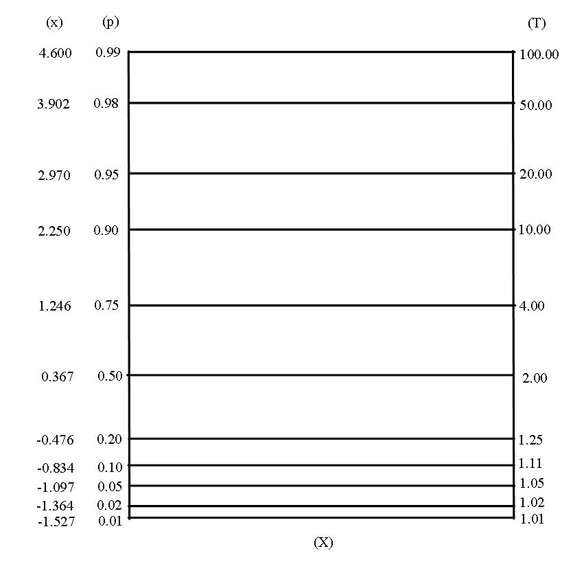
For the probability paper, the iterated logarithms can be built on one of the scales of the paper so that we need only to plot \(\mathrm{\left( x, \Lambda \right) . }\) We do not have only scales for \(\mathrm{ x}\) and \(\mathrm{ \Lambda }\) but also for \(\mathrm{ T}\) as been in the usual probability paper that follows.

Figure 4.1. Gumbel maxima probability paper

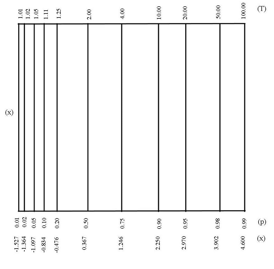
The next figure illustrates the reverse probability paper where the scales of \(\mathrm{ \left( x, \Lambda \right) }\) are exchanged, as engineers often do.

Figure 4.2. Gumbel maxima probability paper (reverse)

So far we have ignored the problem of determining an estimate of \(\mathrm{ \Lambda \left( \left( x_{i}^{’}- \lambda \right) / \delta \right) }\) to plot. One could use, \(\mathrm{~i/n }\) as plotting position to go with \(\mathrm{x_{i}^{’}~, }\) the i^th order statistic in a sample of \(\mathrm{​​n}\) , which is the usual plotting position for the sample distribution function, used for example in the Kolmogorov-Smirnov bounds. This is equivalent to estimating \(\mathrm{ \Lambda \left( \left( x_{i}^{’}- \lambda \right) / \delta \right) }\) as the proportion of \(\mathrm{x_{j}^{’}~s }\) less than or equal to \(\mathrm{x_{i}^{’}.}\) Since 1 (and also 0) do not appear on the \(\mathrm{\Lambda }\)-scale, we cannot plot \(\mathrm{\Lambda \left( \left( x_{n}^{’}- \lambda \right) / \delta \right) . }\) If we estimate \(\mathrm{ \Lambda \left( \left( x_{i}^{’}- \lambda \right) / \delta \right) }\) by\(\mathrm{~ \left( i-1 \right) /n }\), the proportion of \(\mathrm{x_{j}^{’} \,s}\) less than \(\mathrm{x_{i}^{’} }\), we cannot plot \(\mathrm{\Lambda \left( \left( x_{1}^{’}- \lambda \right) / \delta \right) }\). As a compromise it was suggested to “split the difference” and use \(\mathrm{\left( i - 1/2 \right) /n }\) as the estimate of \(\mathrm{ \Lambda \left( \left( x_{i}^{’}- \lambda \right) / \delta \right) }\). Another procedure is to use the mean value of \(\mathrm{ \Lambda \left( \left( x_{i}^{’}- \lambda \right) / \delta \right) }\) as a plotting position, which leads to the value \(\mathrm{ i/ \left( n+1 \right) .}\) Blom (1958) devoted almost an entire book to the problem of obtaining “optimum” plotting positions, based on the idea of Chernoff and Lieberman (1954) that the plotting position should depend on the quantity to be estimated. For example Blom (1958)(p.145) shows that for the normal distribution, plotting position \(\mathrm{\left( i- 3/8 \right) / \left( n+1/4 \right) = \left( i - .375 \right) / \left( n+.25 \right) }\)leads to a practically unbiased estimate of \(\mathrm{\sigma }\) with a mean square error about the same as that of the unbiased best linear estimate, while the plotting position \(\mathrm{(i-.5)/n }\) leads to a biased estimate of \(\mathrm{\sigma }\) with nearly minimum mean square error.

Note that some symmetry of plotting positions must be verified: if \(\mathrm{p_{i,n} }\) is the plotting position for the \(\mathrm{x_{i}^{’} }\) then we should have \(\mathrm{p_{i,n}+ p_{n+1-i,n}= 1 }\) which does not happen with the plotting positions \(\mathrm{ i/ n }\) and \(\mathrm{\left( i-1 \right) /n }\) but happens with the two other ones. Another perspective, to be used further in the next section, leads to the plotting position \(\mathrm{ p_{i}= \left( i-0.3 \right) / \left( n + 0.4 \right) , }\) also symmetrical; for details see Tiago de Oliveira (1983). Taking  \(\mathrm{p_{i,n}= \left( i+A \right) / \left( n+B \right) }\) the symmetry condition leads to \(\mathrm{B=2A+1 }\) and \(\mathrm{p_{i,n}= \left( i+A \right) / \left( n+1+2A \right) }\) and as \(\mathrm{0<p_{i,n}<1 }\) for each \(\mathrm{i}\) and \(\mathrm{n}\) we must have \(\mathrm{-1<A; }\) for \(\mathrm{A~=-1/2,~A=0,A=3/8 }\) and\(\mathrm{~A=-.3 }\) we obtain the given plotting positions. We have   \(\mathrm{max_{i} \vert \frac{i+A}{n+1+2A}-\frac{i+A’}{x+1+2A’} \vert \leq \frac{ \vert A-A’ \vert }{n}~ }\). Note that for very large \(\mathrm{A}\) all the plotting positions are close to \(\mathrm{1/2}\) which means that it is acceptable to use \(\mathrm{\vert A \vert <1 }\) to have a reasonable spread of the plotting positions in \(\mathrm{\,] 0,1 [ \,; }\) in that case the upper bound \(\mathrm{\vert A-A’ \vert /n }\) of the maximum error is bounded above by \(\mathrm{2/n }\) and is practically irrelevant for sample sizes \(\mathrm{n \geq 50 }\) , and all \(\mathrm{p_{i,n} }\)  are practically equivalent (3) .

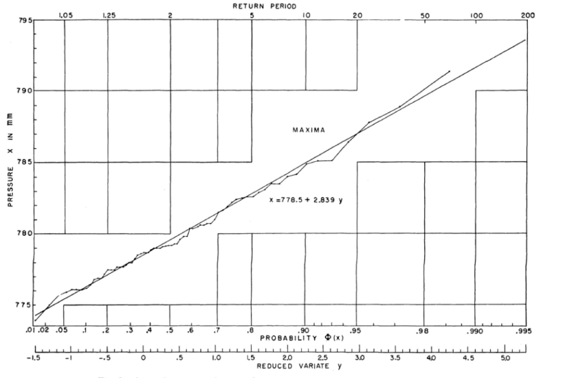
In the graph that follows we will use the classical Gumbel plotting position \(\mathrm{i/ \left( n+1 \right) }\).  Figure 4.3 that follows was taken from Gumbel and Lieblein (1954) and illustrates the procedure for estimating \(\mathrm{\lambda ^{*}=778.5~and~ \delta ^{*} = 2.839}\) for maximum atmospheric pressure (in mm) at Bergen, Norway for the period between 1857 and 1926. If the fitted straight line is extrapolated beyond the fitted values, one would “predict”, for example, that a pressure of \(\mathrm{793~mm }\) corresponds to a probability of 0.994. That is, pressures of this magnitude have less than 1 chance in 100 of being exceeded in any particular year.

Figure 4.3. Annual maxima of atmospheric pressures, Bergen, Norway, 1857-1926 (reverse probability paper)

4 . The use of Gumbel probability paper for quick statistical choice between Weibull, Gumbel and Fréchet distributions for maxima

Here we will describe a graphical technique taken from Tiago de Oliveira (1983). As was shown in the previous section, \(\mathrm{Z}\) being a reduced random variable, the probability paper for Gumbel distribution was made as follows: from \(\mathrm{p= \Lambda \left( z \right) ,}\) which can be written as \(\mathrm{\Lambda ^{-1} \left( p \right) =z, }\) if we note by \(\mathrm{y = \Lambda ^{-1} ( p ) }\) and graduate the y-axis in the functional scale \(\mathrm{p}\), the relation \(\mathrm{p= \Lambda \left( z \right) }\) can be written as the first diagonal \(\mathrm{y =z. }\) In addition, if the true distribution is \(\mathrm{G ( z \vert \theta ) =exp⁡ \{ - \left( 1+ \theta {z} \right) _{+}^{-{1}/{ \theta }} \} ,}\) the von Mises-Jenkinson formula, the relation \(\mathrm{p = \Lambda \left( y \right) =G \left( z \vert \theta \right)}\) may be written as \(\mathrm{y= \Lambda ^{-1} \left( G \left( z \vert \theta \right) \right)}\) and the relation between \(\mathrm{(z,y)(or(z,p))}\) is the curve in the plane \(\mathrm{y=log \left( 1+ \theta {z} \right) / \theta ,~ for~1+ \theta {z}>0. }\)

Let us now return to the plotting positions. If \(\mathrm{p_{i,n} }\) is the plotting position for the order statistic \(\mathrm{z_{i}^{’} ( =~z_{i,n}^{’}}\) with greater rigour) the distance between the plotted point \(\mathrm{ ( z_{i}^{’},p_{i,n}^{’} )}\) and the first diagonal is \(\mathrm{\vert \Lambda ^{-1} \left( p_{i,n} \right) -z’_{i} \vert }\) horizontally or vertically or \(\mathrm{\vert \Lambda ^{-1} \left( p_{i,n} \right) -z’_{i} \vert \sqrt{2}}\) orthogonally.  The distance \(\mathrm{\vert \Lambda ^{-1} \left( p_{i,n} \right) -z’_{i} \vert }\) is minimized in mean if \(\mathrm{\Lambda ^{-1} \left( p_{i,n} \right) }\) is the median of \(\mathrm{z_{i}^{’} }\) (with Gumbel distribution) or \(\mathrm{p_{i,n} }\) is the median of Beta \(\mathrm{\left( i, n-1- i \right) }\)distribution; a good approximation is to take the one given before, \(\mathrm{p_{i,n}=\frac{i-0.3 }{ n+0.4 };}\) note that we are not using the least squares approach but we are minimizing \( \mathrm {\begin{array}{c} \\ \mathrm{max} \\ \mathrm{i} \end{array} \vert \Lambda ^{-1} \left( p_{i,n} \right) -z_{i}^{’} \vert }\).      

Having chosen one of these plotting positions, let us consider the general case, i.e. observations with unknown location and dispersion parameters \(\mathrm{\lambda}\) and \(\mathrm{\delta , z_{i} = \left( x_{i}- \lambda \right) / \delta }\) being the reduces values. Then if \(\chi_{ \mathrm{\theta }}\mathrm{ ( p ) }\) is the \( \mathrm{p}\)-quantile of \( \mathrm{G \left( z \vert \theta \right) , }\) i.e. \( \mathrm{G \left( \chi _{ \theta } \left( p \right) \vert \theta \right) =p, }\)the \( \mathrm{p}\)-quantile of\( \mathrm{~G \left( \left( x- \lambda \right) / \delta \vert \theta \right) }\)is, evidently,\( \mathrm{~ \lambda + \delta \chi _{ \theta } \left( p \right) . }\)Consider then the random variable

\(\mathrm{v=\frac{x- \left( \lambda + \delta ~ \chi _{ \theta } \left( r \right) \right) }{ \left( \lambda + \delta ~ \chi _{ \theta } \left( s \right) \right) - \left( \lambda + \delta ~ \chi _{ \theta } \left( r \right) \right) }=\frac{z- \chi _{ \theta } \left( r \right) }{ \chi _{ \theta } \left( s \right) - \chi _{ \theta } \left( r \right) } }\)

with \( \mathrm{0< r< s<1; }\) \( \mathrm{v }\) is obviously independent of the location and dispersion parameters.

Clearly we are going to plot estimated  \( \mathrm{v_{i }^{'} }\) where the \( \mathrm{r }\) and \( \mathrm{s }\) quantiles are estimated by the sample quantiles by \( \mathrm{x_{ \left[ nr \right] +1}^{’} }\) and  \( \mathrm{x_{ \left[ ns \right] +1}^{’} }\).

The relation \( \mathrm{p= \Lambda \left( y \right) =G \left( z \vert \theta \right)}\) can then be written as \( \mathrm{y= \Lambda ^{-1} (G( \chi _{ \theta }(r)+ (\chi _{ \theta }(s)- \chi _{ \theta }(r))v|\theta=y_\theta(v) , }\) for \(\mathrm{r}\) and \(\mathrm{s}\) fixed. Taking \(\mathrm{v=0}\) and \(\mathrm{v=1}\) we see that all curves \(\mathrm{y_{ \theta } \left( v \right) }\) pass through the points \(\mathrm{\left( 0, \chi _{0} \left( r \right) \right) }\) and \(\mathrm{\left( 1, \chi _{0} \left( s \right) \right) }\), or \(\mathrm{\left( 0, r\right)}\) and \(\mathrm{\left( 0, s \right)}\) if we use the functional scale for \(\mathrm{y}\). Thus between \(\mathrm{v=0}\) and \(\mathrm{v=1}\) the curves \(\mathrm{y_\theta\,(v)}\) will with difficulty be separated from the first diagonal, chiefly taking into account that the plotted points, even using real and not estimated reduced observations, do not fall exactly on the first diagonal for Gumbel distribution. In summary, the points between \(\mathrm{v=0}\) and \(\mathrm{v=1}\) are lost for separation of models; it is, thus, natural to use about \(\mathrm{1/3}\) of the observations for the zone \(\mathrm{v \in \left[ 0,1 \right] }\) and \(\mathrm{2/3}\) outside; a smaller percentage in this zone would introduce instability in the implicit estimation of \(\mathrm{\lambda }\) and \(\mathrm{\delta }\) by the quantiles, as the denominator would be small.

With this rule of thumb, we have taken \(\mathrm{ \chi _{0} \left( r \right) =0 }\) and, \(\mathrm{ \chi _{0} \left( s \right) =1 }\),  or \(\mathrm{r = \Lambda ^{-1} \left( 0 \right) = e^{-1}=0.3678794 }\) and \(\mathrm{s = \Lambda ^{-1} \left( 1 \right) = exp \left( - e^{-1} \right) = 0.6922006 }\) (note that, as said before,\(\mathrm{~~r \approx 1/3~ }\) and\(\mathrm{s \approx 2/3); }\) practically we can take \(\mathrm{r=0.368 }\) or even \(\mathrm{r=0.37}\) and \(\mathrm{s=0.692}\) or even \(\mathrm{s=0.69.}\)

Let us now compute the curves \(\mathrm{y_{ \theta } \left( v \right) . }\) As \(\mathrm{\chi _{ \theta } ( p ) =\frac{ \left( -log~p \right) ^{- \theta }-1}{ \theta } }\) and so \(\mathrm{\chi _{ \theta } \left( e^{-1} \right) =0~ }\)and  \(\mathrm{\chi _{ \theta } \left( exp ( -e^{-1} ) \right) = \left( e^{ \theta }-1 \right) / \theta }\) we get

\(\mathrm{y_{ \theta } \left( v \right) =\frac{log \left( 1+ \left( e^{ \theta }-1 \right) v \right) }{ \theta } }\)

which is evidently defined when \(\mathrm{1+ \left( e^{ \theta }-1 \right) v>0; }\) note that \(\mathrm{y_{ \theta } \left( v \right) }\) is convex for \(\mathrm{\theta <0 }\) (Weibull model) and concave for \(\mathrm{\theta>0 }\) (Fréchet model), \(\mathrm{y_0 ( v ) }\) (Gumbel model) being a straight line.

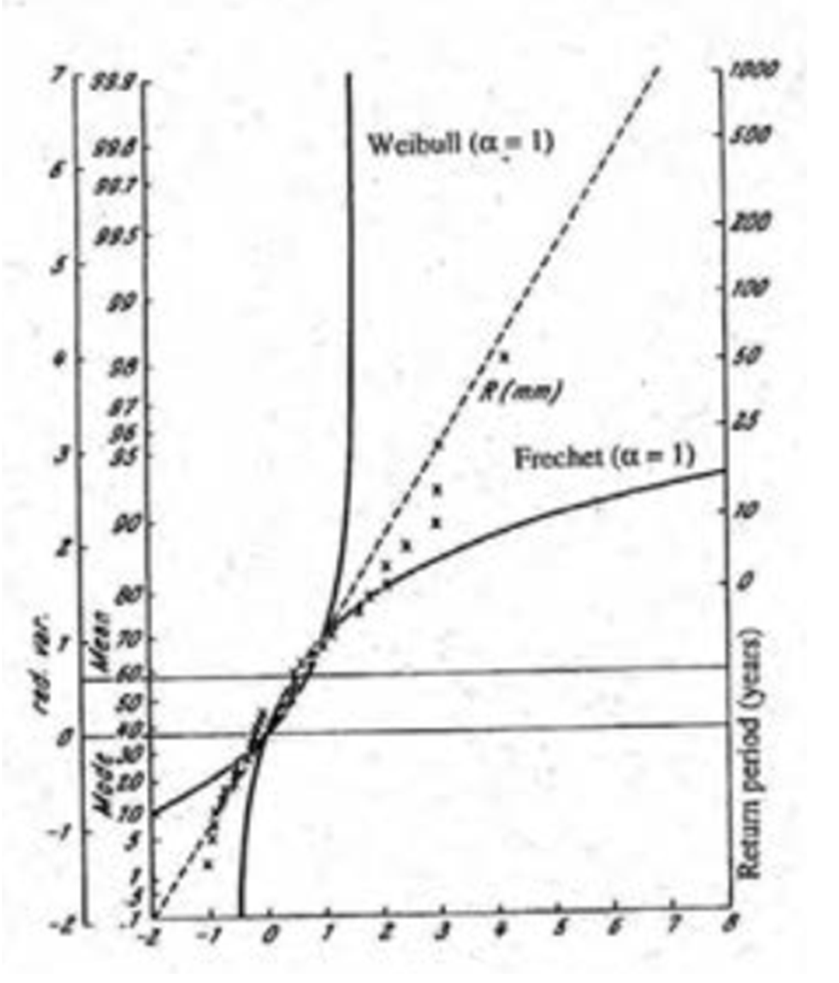
Thus in a Gumbel probability paper we plot a bundle of curves \(\mathrm{\left( v,~y_{ \theta } \left( v \right) \right) }\) for different values of  \(\mathrm{\theta }\) and the quick statistical choice is made according to the location of the plotted points \(\mathrm{\left( v_{i}^{’},p_{i} \right) }\) close to the diagonal (Gumbel distribution) or in the Fréchet or Weibull zones as shown in  the Figure 4.4. Estimation of the parameters is to be made by the analytical methods of the next three chapters.

As an example consider the Table 1 of maximum wind velocities in km/h between 1941-1970 in Lisbon.

The values of the maximum likelihood estimators are \(\mathrm{\hat{\lambda }= 94.71~}\) and \(\mathrm{\hat{\delta } = 12.49; }\) the \(\mathrm{1/e}\)-quantile and \(\mathrm{exp\,(-1/e})\)-quantile needed for computation of the \(\mathrm{v_{i}^{'}}\) are \(\mathrm{Q\left( .367 \right) = 96.0 }\) and \(\mathrm{Q ( .692 ) =108.0; }\) we took, as said before \(\mathrm{p_{i}=i/ \left( n+1 \right) . }\)

         As regards m^th extreme, the simplest way is to try the statistical choice for maxima (or minima) because then the limiting distribution is well known and was given in Part-1.

Figure 4.4

Plotting of \(\mathrm {(v'_i,p_i)}\) for the maximum wind velocities in km/h in Lisbon, 1941-1970; Fréchet and Weibull zones shown.

5 . Simple statistical choice between the extreme models

We will use a simple statistic proposed in Gumbel (1965) for the study of the Fréchet distribution. In Tiago de Oliveira and Gomes (1984) we developed the asymptotic theory of this statistic for all distributions. Let us denote for a sample \(\mathrm{\left( x_{1},…,x_{n} \right) ,}\) from the distribution \(\mathrm{G ( z \vert \theta ) ~by~~x_{1}^{’}=min ( x_{i} ) ,x_{ \left[ n/2 \right] +1}^{’}=med\,\{X_i\}\,\,and\,\,x_{n}^{’}=max\,\{X_i\}}\) the maximum, the medium and the minimum of the sample. We consider the statistic

\(\mathrm{Q_{n}=Q_{n, \theta }=\frac{x_{n}^{'}-x_{[n/2]+1}^{'}}{x_{[n/2]+1}^{'}-x_{1}^{'}}=\frac{max\{x_i\}-med\{x_i\}}{med\{x_i\}-min\{x_i\}}}\)

which is, evidently, location and dispersion parameter-free.

We have shown in Tiago de Oliveira and Gomes (1984) that if \(\mathrm{\theta =0, G ( z \vert 0^{+} ) =G ( z \vert 0^{-} ) = \Lambda \left( z \right) , }\) there exist \(\mathrm{\beta _{n,0} }\) and \(\mathrm{\alpha _{n,0}>0 }\) such that \(\mathrm{~~\frac{Q_{n}- \beta _{n,0}}{ \alpha _{n,0}}\stackrel{\mathrm{w}}{\rightarrow} \Lambda \left( z \right) ; }\) a choice is \(\mathrm{\beta _{n,0}=\frac{log~n+log\,log\,2}{log~log~n-log\, log\,2}, \alpha _{n,0}={1}/{log}\,log~n; }\) if \(\mathrm{\theta >0, G \left( z \vert \theta \right) = \Phi _{1/ \theta } \left( \theta z+1 \right) , }\) there exist \(\mathrm{\beta _{n, \theta }}\) and \(\mathrm{\alpha _{n,\theta}>0 }\) such that \(\mathrm{\frac{Q_{n}- \beta _{n, \theta }}{ \alpha _{n, \theta }}\stackrel{\mathrm{w}}{\rightarrow}G (z\vert \theta ) = \Phi _{1/ \theta } \left( \theta z+1 \right); }\) a choice is \(\mathrm{\beta _{n, \theta }=\frac{n^{ \theta }- \left( log\,2 \right) ^{- \theta }}{ \left( log\,2 \right) ^{- \theta }- \left( log\,n \right) ^{- \theta }}~;~ \alpha _{n, \theta }= \theta \left( n\,log\,2 \right) ^{ \theta } }\) or more simply   \(\mathrm{\beta ’_{n, \theta }= \left( n~log⁡~2 \right) ^{ \theta }, \alpha ’_{n, \theta }= \theta ~ \beta ’_{n, \theta }~;~if~ \theta <0, G \left( z \vert \theta \right) = \Psi _{-1/ \theta } \left( - \theta z-1 \right) , }\) there exist \(\mathrm{\beta _{n, \theta } }\) and \(\mathrm{\alpha _{n, \theta } > 0 }\) such that \(\mathrm{ \frac{Q_{n}- \beta _{n, \theta }}{ \alpha _{n, \theta }}\stackrel{\mathrm{w}}{\rightarrow}1-\Lambda(-z) }\); a choice is \(\mathrm{\beta _{n, \theta }=\frac{n^{ \theta }- \left( log~2 \right) ^{- \theta }}{ \left( log~2 \right) ^{- \theta }- \left( log~n \right) ^{- \theta }}~; \alpha _{n, \theta }=- \theta \left( log~2 \right) ^{- \theta } \left( log~n \right) ^{ \theta -1}}\) or even more simply for \(\mathrm{\theta <1, \beta ’_{n, \theta }= ( \frac{log~n}{log~2} ) ^{ \theta } }\) and similarly  \(\mathrm{\alpha ’_{n, \theta }= \alpha _{n, \theta }=-\frac{ \theta }{log~n}~ \beta ’_{n, \theta }. }\)

Two intuitive conclusions may be drawn from these results:

1. There is a “discontinuity” between \(\mathrm{\theta \geq 0 }\) and \(\mathrm{\theta <0; }\) for \(\mathrm{\theta \geq 0 }\) the influent term is the maximum but for \(\mathrm{\theta <0 }\) ; the influent term is the minimum; this explains, to a certain extent, why we cannot have a simple common expression for \(\mathrm{\beta _{n,\theta} }\) and \(\mathrm{\alpha _{n,\theta} }\).
2. As for \(\mathrm{\theta \geq 0, \alpha _{n, \theta } \rightarrow \infty }\) and for \(\mathrm{\theta <0, \beta _{n, \theta } \rightarrow \infty0 }\) it seems natural to decide for the Fréchet distribution \(\mathrm{\left( \theta >0 \right) }\) if \(\mathrm{Q_n }\) is large and for the Weibull distribution \(\mathrm{\left( \theta <0 \right) }\) if \(\mathrm{Q_n }\) is small; then the decision rule will be:

Choose \(0 < b < a <+ \infty \) and decide for the Gumbel distribution when \(b \leq \frac{Q_{n}- \beta _{n,0}}{ \alpha _{n,0}} \leq a,\) for the Fréchet distribution when  \(\frac{Q_{n}- \beta _{n,0}}{ \alpha _{n,0}}>a, \) and for the Weibull distribution when \(\frac{Q_{n}- \beta _{n,0}}{ \alpha _{n,0}}<b, \) where  \(\beta _{n, \theta }=\frac{log\,n+log\,log\,2}{log\,log\,n-log\,log\,2} \) and \(\alpha _{n, \theta }= \left( log\,log\,n \right) ^{-1}. \) 

Let us compute, for \(\mathrm{b<a,}\) the probabilities of correct decision; using the Khintchine convergence of types theorem:

\(\mathrm{1 ) ~~ \theta =0:~~~~~~~~Prob \{ b \leq\,\frac{Q_{n}- \beta _{n,0}}{ \alpha _{n,0}}<a \} \rightarrow \Lambda \left( a \right) - \Lambda \left( b \right) ; }\)

\(\mathrm{2 ) ~~ \theta >0:~~~~~~~~Prob \{ \frac{Q_{n}- \beta _{n,0}}{ \alpha _{n,0}}> a \} \rightarrow 1-G \left( -1/ \theta \vert \theta \right) =1:}\)

\(\mathrm{3 ) ~~ \theta <0:~~~~~~~~Prob \{ \frac{Q_{n}- \beta _{n,0}}{ \alpha _{n,0}}< b \} \rightarrow 1-G \left( -1/ \theta \vert \theta \right) . }\)

The technique is thus consistent in the usual sense, whatever \(\mathrm{0 < b < a <+ \infty }\) may be; in fact if the decision technique is such that for \(\mathrm{\theta=0}\) the limit probability of correct decision is \(\mathrm{\Lambda \left( a \right) - \Lambda \left( b \right) ,}\) but if \(\mathrm{​​​​\theta \neq 0 }\) the limit probability of correct decision is 1. We could improve the situation by putting the significance level \(\mathrm{\alpha _{n}=1- \left( \Lambda \left( a_{n} \right) - \Lambda \left( b_{n} \right) \right) \rightarrow 0 }\) with convenient restrictions in \(\mathrm{b_n }\) and \(\mathrm{a_n }\). But this does not seem to be needed because it is well known that for large \(\mathrm{\alpha}\) (i.e, for small \(\mathrm{\theta}\) in von Mises-Jenkinson form) both the Fréchet and the Weibull distributions are very close to the Gumbel distribution. Following on from the previous remark, it seems natural to solve only the statistical trilemma \(\mathrm{\left( \theta <0, \theta = 0~or~ \theta > 0 \right) }\) and not a statistical dilemma or one-sided test of hypothesis of \(\mathrm{\theta =0~vs.~ \theta >0~or~ \theta = 0~vs.~ \theta <0. }\) The latter would correspond to the partial acceptance of \(\mathrm{\theta \geq 0~or~ \theta \leq 0 }\) which lead to a one-sided test as a consequence of assuming stronger previous knowledge or a stronger plausibility. Thus we will not deal with one-sided tests.

It remains now to obtain the one equation for \(\mathrm{(b,a)}\) and the best seems, from what has been said, that the length of the Gumbel decision interval \(\mathrm{a-b}\) should be the smallest possible with the condition \(\mathrm{\Lambda \left( a \right) - \Lambda \left( b \right) = 1- \alpha . }\) The use of Lagrange multipliers gives the equations

\(\mathrm{\Lambda \left( a \right)- \Lambda \left( b \right) =1- \alpha }\)

\(\mathrm{\Lambda ^{’} \left( a \right) = \Lambda ^{’} \left( b \right) . }\)

The values corresponding to the usual significance levels are:

Examples of quick exploration of data, as well as the analysis of univariate models and statistical choice, can be found in the “Some Case Studies” chapter.

6 . Footnotes

(1)     Recall that Poincaré (a mathematician) said Lippman (a physicist) told him that physicists used normal distribution supposing it to be a theorem, while mathematicians studied it supposing it to be experimentally verified.

(2)  Recall the justification of the Poisson distribution used by “Student” for the counts of particles in a haemacytomaters.

Tables

Figures

References

1.
Blom, G., 1958. Statistical Estimation and Transformed Bet-Variables, Wiley, New York.
Gumbel, E. J., 1958. Statistics of Extremes, Columbia University Press, New York.
9.
Gumbel, E. J., 1962. Statistical theory of extreme values (main results). in ContributionstoOrder Statistics, Ahmed E. Sarhan and Bernard G. Greenberg eds., 56-93, Wiley, New York.
10.
Gumbel, E. J., 1965. A quick estimation of the parameters in Fréchet distribution. Rev. Int, Statist. Inst., 33, 349-363.
Thom, H. C. S., 1960. Distribution of extreme winds in the United States. J. Structural Div., Proc. ASCE, 86.
13.
Thom, H. C. S., 1971. Asymptotic extreme-value distributions of wave heights in the open ocean. J. Marine Res., 29, 19-27.
14.
Tiago de Oliveira, J., 1977. Asymptotic distributions of univariate and bivariate m-th extremes. in Recent Developments in Statistics, J. R. Barra et al. eds., 613-619, North-Holland, Amsterdam.
15.
Tiago de Oliveira, J., 1983. Gumbel distribution. in Encyclopedia of Statistical Sciences III, N. L. Johnson and S. Kotz eds., 552- 558, Wiley, New York.
16.
Tiago de Oliveira, J., and Gomes, M. I., 1984. Two test statistics for choice of univariate extremes models. in Statistical Extremes and Applications, J. Tiago de ed., D. Reidel, Dordrecht.
17.
Weibull, W., 1939. A statistical theory of the strength of materials. Proc. Roy. Swed. Inst. Eng. Res., 151, Stockholm.
we get
and
and  we get the same result for minima with