Keywords

Valuation , Land use , Khulna , GIS , Ecosystem services

1 . INTRODUCTION

The goods and services those humans and other living organisms obtain directly or indirectly from natural systems are referred to as ecosystem services (MEA, 2005; Costanza et al., 2014). The urban ecosystem provides many functions such as food and water, temperature and climate control, waste treatment, soil formation, provision of habitant, production of atmospheric oxygen, management of urban heat islands, etc. (Xie et al., 2017; Langemeyer et al., 2016). A sound ecosystem contributes to livable and green improvement (Rahman and Szabo, 2021). Despite the exceptional provision of services provided by ecosystems to nature and living-being, anthropogenic factors have the potential to modify ecological surroundings and natural ecosystems by altering the formation and arrangement of the usage of land (Belay et al., 2022).

Urban ecosystem services are under threat as a result of fast urbanization, continuous population increase, migration, climate change, and industrialization and the present urban ecosystem services may not be able to survive such strain (Liu et al., 2019). With fast economic development and population expansion during the last five decades, at least two-thirds of ecosystems have degraded resulting in a large drop in ES and severe loss in biodiversity (Wang et al., 2022). The decline of urban environment resources is a clear impediment to meeting the MDGs [Millennium Development Goals] (Chen et al., 2020).

Urban ecosystem services are diminishing because of anthropogenic activities and natural occurrences (Escobedo et al., 2011; De Araujo Barbosa et al., 2016; Liu et al., 2020). Land use and land cover changes are among the most significant influences that overrun or degrade the capacity of environmental processes and services (Li et al., 2007; Liu et al., 2014; Islam et al. 2016). Because of increased urbanization and population mobility, the pace and degree of the changes in land use are occurring at a higher rate than in the past (Lambin et al., 2011). Due to the rapid pace of development efforts and interventions, the conversion of land from natural ecosystems to urban areas has resulted in the loss of ecosystem services (Dewan and Yamaguchi, 2009; Xia et al., 2020). For example, conversion from wetland to built-up is responsible for urban flooding because of heavy rainfall (Zhao et al., 2019).

The field of ecosystem services was first explored on a global scale in the early 1970s (Guo et al., 2022). Since then, numerous types of research have now been conducted to investigate how land utilization and ground cover modification affect ecological services. (Wang et al., 2018; Jiang et al., 2020) and the majority of them are concerned with evaluating how sensitive ecosystem service is to land use and land cover modification (Spake et al., 2017). There are four ways to evaluate ecosystem services, such as the revealed preferential process, stated preferential practice, cost-dependent method and benefits transfer technique (Talberth, 2015). The Benefit Transfer Method, developed in 1997 by Costanza, is the most widely used approach for valuing ecosystem services worldwide. The benefit transfer technique to Ecosystem Service Value (ESV) has been criticized for failing to account for local variability, which is a fundamental aspect of the environment (Baveye et al., 2013; Horlings et al., 2020). Despite these disadvantages, the Benefit Transfer Process is applied to assess the worth of ecosystems in data-poor locations (Costanza et al., 2014). Being inspired by the work of Costanza et al. (2014), several efforts had been undertaken to quantify the value of changing ecosystem services such as Kreuter et al. (2001), Liu et al. (2011) Kindu et al. (2016), Yi et al. (2017), Tian et al. (2021), Tolessa et al. (2021), Anley et al. (2022), etc.

Bangladesh has also seen enormous land-use changes in recent decades as a result of growing urbanization and population pressures (Hasan, 2017; Mukhopadhay, 2018). Urbanization has taken over rural areas and it is projected that 199908 hectares of agricultural land are urbanized (Sayed and Haruyama, 2015). In Bangladesh, a number of research projects have been conducted to evaluate the impact of land use shifts and the significance of alterations in ecosystem services (Dewan et al., 2010; Khan et al., 2014; Islam et al., 2015; Islam et al., 2016; Hasan et al., 2017; Mukul et al., 2017; Hasan et al., 2020; Dey et al., 2021) but those are very limited, especially the use of satellite image-derived land use and ground cover shift for the assessment urban ecosystem service. Land-use changes are pronounced in Bangladesh’s southwest coastal areas (Khan et al., 2014). Khulna conurbation, both a divisional city and one of Bangladesh’s coastal zones, has seen significant changes in its land cover over the last several decades because of accelerated urbanization, economic expansion, rising mean sea level, climate emergencies, and natural catastrophic events (Moniruzzaman et al., 2018). Land-use change in urban areas is responsible for slimming down agricultural land and wetland. Therefore, the land turning into urban areas has detrimental effects on several ecosystem services of this city such as provisioning services (rice, fisheries production, and livestock), regulating services (natural drainage system), and cultural services (aesthetic view). Research on land use change and valuation of ecosystem services in Khulna is scarce; however, there are some studies in southwest coastal regions. For instance, Akber et al. (2018) investigated the outcome of land use changes on ecosystem services in the Khulna, Satkhira, and Bagerhat districts. In addition, as part of the coastal region research, Hoque et al. (2022) also examined the effects of land use change on the ecosystem service functions of Khulna. As a result, this is the first research of its type to use satellite images to quantify the impact of land use shifts on ecosystem services in Khulna Conurbation. The specific objectives of this study: i) to explore land use scenarios in the years 1987, 1996, 2007, and 2018 of Khulna conurbation; ii) to evaluate the worth of individual ecosystem services; iii) to determine the influence of land use change on ecosystem services in the study region. The findings should be beneficial in developing remuneration for environmental services, and they should have a favorable impact on natural resource management and urban development strategies.

2 . METHODOLOGY

2.1 Study Area

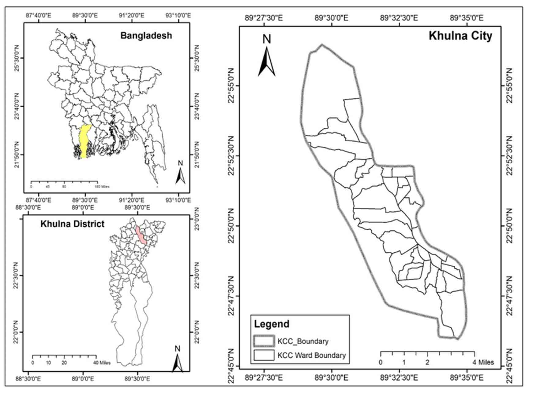
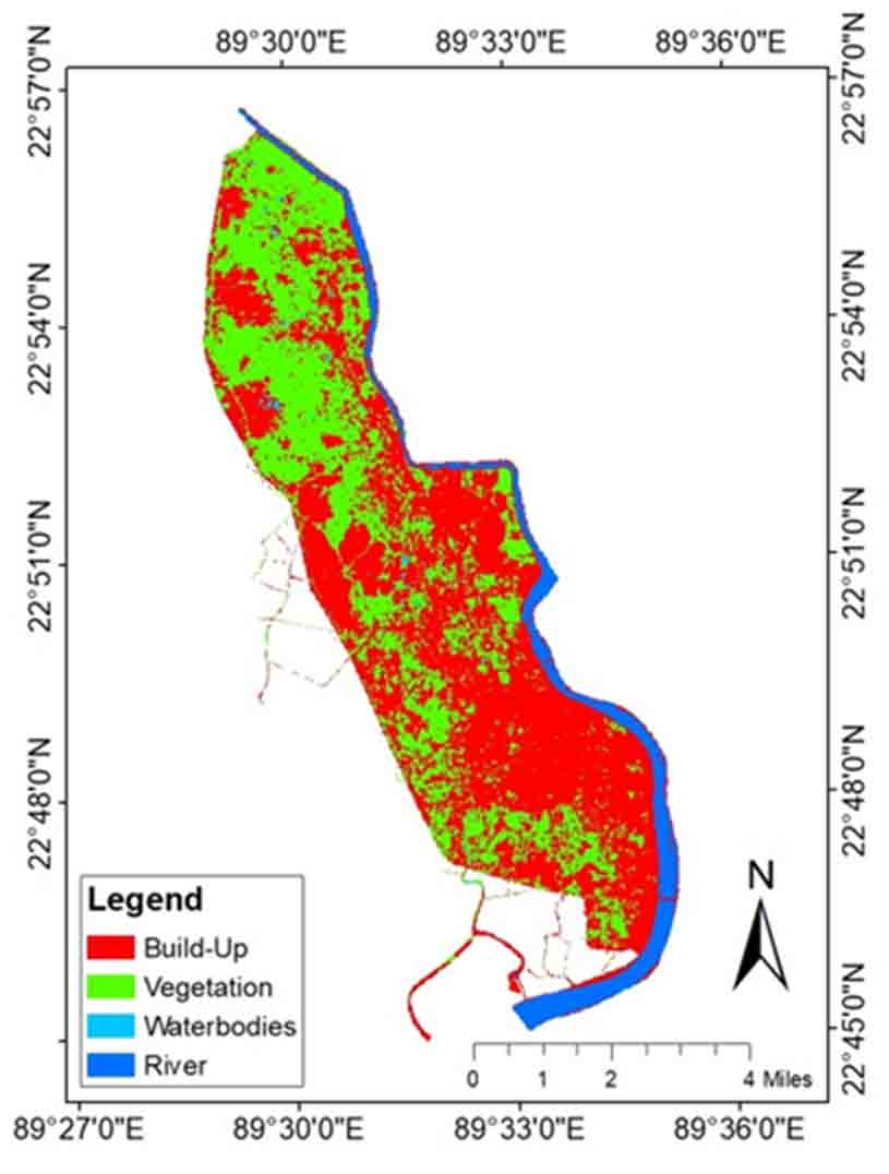
The research was carried out in the Khulna Conurbation, formally known as Khulna City Corporation- KCC (Figure 1), is situated on the Bhairab-Rupsha River’s bank and has been the main center of commerce, manufactory, administration, health, and education in the southwest region (Haque et al., 2020).

Figure 1. Study Area

This city boasts an excellent transit system and a diverse range of urban facilities and services, resulting in a substantial influx of citizens from neighboring cities and places. This land modification is taking underway to accommodate the additional arrivals (Haque et al., 2020). Khulna is bordered on the north, east, south, and west by the Bhairab River, Fultala Upazilla, Rupsha River, and Dumuria Upazilla (BBS, 2022).

The total area of the city is 6478 ha. Khulna Conurbation comprises 31 wards within 5 Thanas with a population of 1.5 million (Morshed et al., 2022). There are about 528 kilometers of drainage networks in the KCC area. There are six regulators and eight gates that let storm water out of Khulna City Corporation (Zannat, 2012). Khulna has an average temperature of 26.37 °C and it has increased by 0.005 °C/year in the last few decades. There is also 1630 mm of precipitation annually. The average elevation of the study area is about 1.8 meters above sea level. This region experiences a tropical monsoon climate, with cold winters and humid, scorching summers (Mondal et al., 2017).

2.2 Satellite Image Acquisition and Land Classification

The remote sensing method is one of the most important methods of identifying land use features with multispectral satellite imagery. The methods for classifying remotely sensed images are supervised and non-supervised (Kafy et al., 2020). Due to the unavailability of Landsat images for the year 1985, Landsat satellite images of 1987, 1996, 2007, and 2018 were analysed to determine the land-use changes (Table 1). The satellite imagery was sourced from the U.S. Geological Survey’s official website. In order to eliminate the possibility of seasonal variations between land use change seasons, Landsat images were all downloaded for the dry period (Johansen et al., 2015; Birhanu et al., 2019; Anley et al., 2022). As there is no rain in the dry season, this guarantees that there are water bodies in fact. The projection system was Universal Transverse Mercator (UTM).

The supervised classification techniques were used to classify the present and past land use of the research area. To prevent any interference with the spectrum information, radiometric augmentation of the pictures was not performed before hybrid categorization (Akber et al., 2018). Similar techniques were applied in the previous studies (Zhaoa et al., 2004; Zang et al., 2011; Rawat and Kumar, 2015; Temesgen et al., 2018; Sumari et al., 2020). 

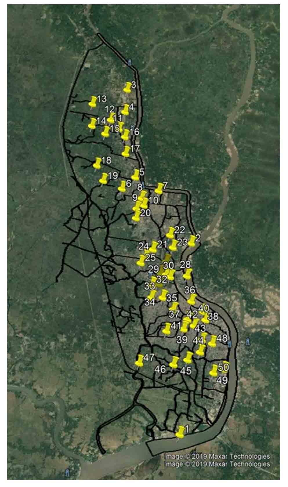
This study classified land use into four distinct sub-categories including Built-up Area (Residential zone, mixed zone, industry, transport), Water Bodies (Permanent open water, Streams, Khal), Vegetation (Park, Stadium, Urban Green, Crop Field), and Rivers (Lakes and Rivers) as those are the main types of land uses in the study area. As Khulna Conurbation is an urban area, these are the primary land categories in the city. These usages of land were selected considering the biomes close to these land-use types to calculate the ecosystem values (Rahman and Szabo, 2021). Estimating the uncertainties in land use change must be handled carefully. Therefore, a ground-truthing survey which is a remote sensing field verification technique was utilized to evaluate the accuracy of the categorized map (Islam et al., 2016). A set of 50 ground-truthing locations were selected for field verification of as much land area as possible. Based on the ground-truthing information, a confusion matrix was constructed to illustrate the classification’s overall precision as a percentage of categorized land use versus actual land use (Rotich et al., 2022).

2.3 Assessment of Ecosystem Services

In recent years, numerous research projects have been conducted on the quantification of ecosystem services. Among them, the ecosystem service assessment method suggested by Costanza et al. (1997) is regarded as the most reliable technique for evaluating the economic worth of ecosystem services. For the purpose of calculating ecosystem service values, 17 ecosystem services were identified across 16 biomes. The methodology of Costanza et al. (1997) has been subject to some criticism due to inaccurate estimations of agricultural units and uncertainty however, it provides the most extensive set of initial estimates for the valuation of ecosystem services (Rahman and Szabo, 2021). As a result, we employed this technique in our study to value ecosystem services in Khulna Conurbation.

Each land use type was compared to distinct biomes found in the global ecosystem to assess ecosystem services. The valuation coefficient in the most ideal biome was utilized as a substitute for each type. In this study, the urban biome for ‘built-up area’, cropland for ‘vegetation’, wetland biome for ‘water bodies’, and river or lakes for ‘river’ was used. Then the updated value of world ecosystem services was applied.  Land use patterns, corresponding biome, and value coefficient are included in (Table 2).

The ecosystem services value was determined by applying the following formula (Long et al., 2014; Arowolo et al., 2018; Liu et al., 2020).

\(ESV= ∑(Ak× VCk)\)           (1)

Where, ESV is the estimated ecosystem services value, AK  is the area (ha) and VCK  is the value coefficient for each land use category. We analysed the differences between the projected ecosystem services value for each land use category in 1987, 1998, 2007, and 2018 to determine the change in ecosystem service value.

2.4 Coefficient of Sensitivity

This study looked at how much each piece of land was worth compared to other parts of the world’s biomes. There may be some ambiguities in this, and they may not be precisely matched. As a result, the coefficient values used to compute ecosystem services value are subject to uncertainty. For this reason, sensitivity analysis must be conducted to determine the extent to which absolute ecosystem service value is dependent on a variation in the coefficient value of a particular land use type. The coefficient of sensitivity (CS) is used to evaluate the performance of biome portrayal and the relative value of the CS in different land use categories. As a result, sensitivity analysis is required to establish the degree of reliance of total ecosystem services value on a shift in the coefficient value of certain land use nature (Wang et al., 2020). The formula used to calculate the CS is as follows (Tolessa et al., 2017; Akber et al., 2018).

\(CS=((ESVj-ESVi)/ESVi)/((vCjk-vCik)/vCik)\)         (2)

Where, ESV is the estimate of ecosystem services value, \(vC\)  is the value component, ‘i’ and ‘j’ represent the original and adjusted values, respectively, and ‘k’ is the land use category.

The ecosystem value ratios for each land use were modulated by a margin of ± 50% (Akber et al., 2018). The coefficient of sensitivity is the ratio between the change in the estimated ecosystem services value and the change in the modified valuation coefficient (Li et al., 2007).  If the difference is less than 1, the estimate of ecosystem service is flexible and reliable; if it’s more than 1, it’s not (Zhao et al., 2004). If the proxy representation and its estimated ecosystem service value are rigid in relation to the value coefficient, then it is reliable.

3 . RESULTS

3.1 Land Use Modification Analysis

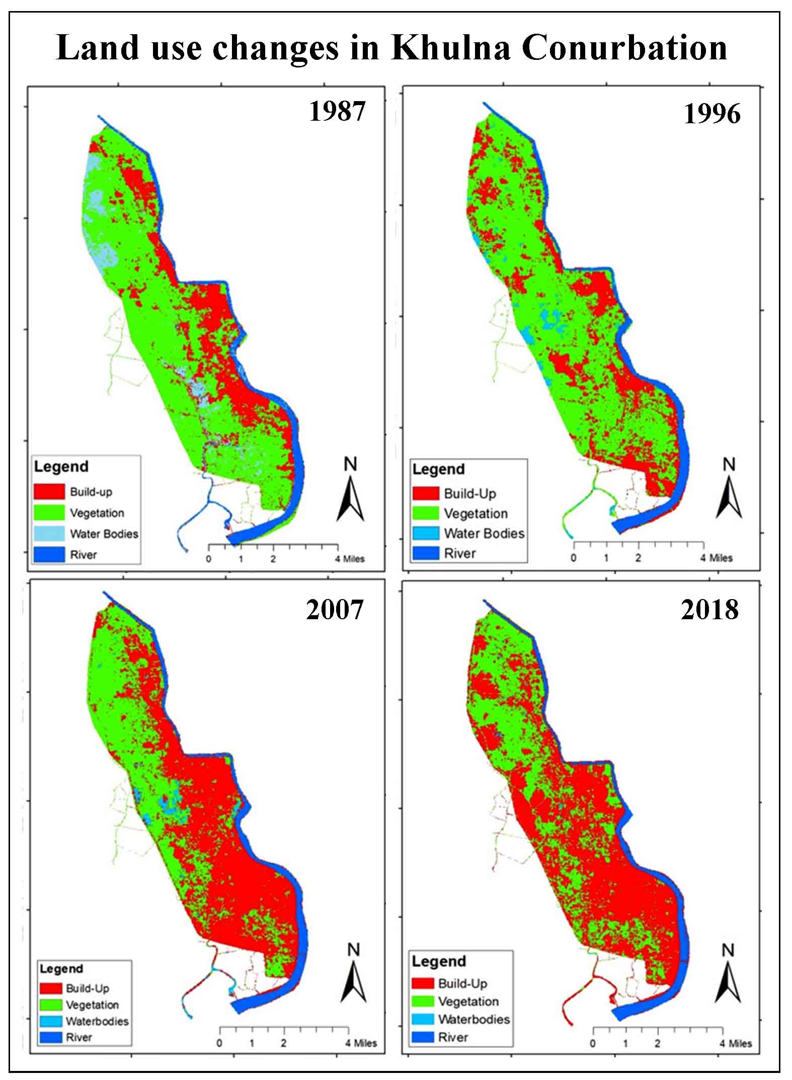
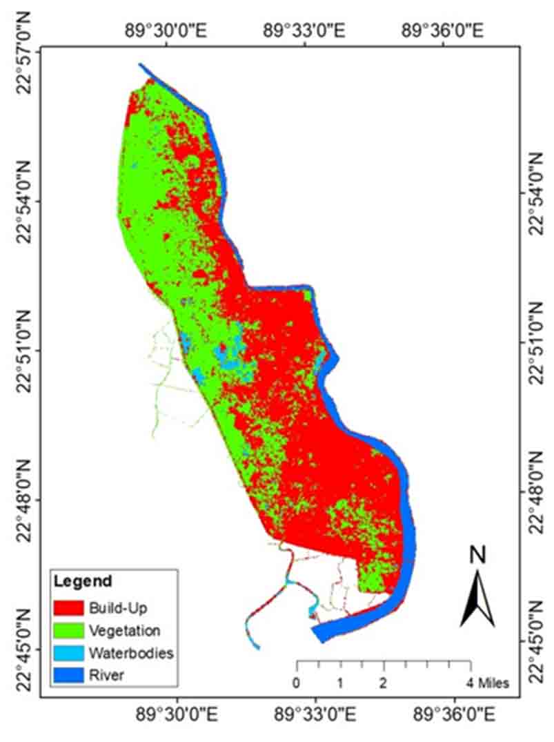
Land use classification was carried out using cloud-free Landsat images of the research area from the years 1987, 1996, 2007, and 2018, which was presented in Figures 2 and 3. The number of changes in each type of land was shown in Table 3.

Figure 1. Study Area

Figure 3. Land use changes: 1996

Figure 4. Land use changes: 2007

Figure 5. Land use changes : 2018

A significant increase was shown in the built-up or settlement area. In 1987, the total built-up area was 1342 ha and in 2018 it was 4332 ha of land which was more than three times. The built-up area grew by 223% between 1987 and 2018 due to the rapid growth of the city, particularly in the northwest and mid-city areas. During this time, the vegetation, water bodies, and river area all showed a downward tendency. The vegetation area decreased from 5716 ha to 3597 ha during the period from 1987 to 2018. Overall, 37% of vegetation area was removed within 31 years because of urban sprawling.

The wetland area decreased from 940 ha to 172 ha from 1987 to 2018. The reduction was driven by the expansion of the developed area specially the construction land. The water body area was also replaced by vegetation or agricultural land but the amount was less than the built-up area. The river area decreased from 784 ha to 692 ha from 1987 to 2018 due to the expansion of the built-up area, dumping of waste into the river, and adjacent canal, which reduced the navigability of the river.

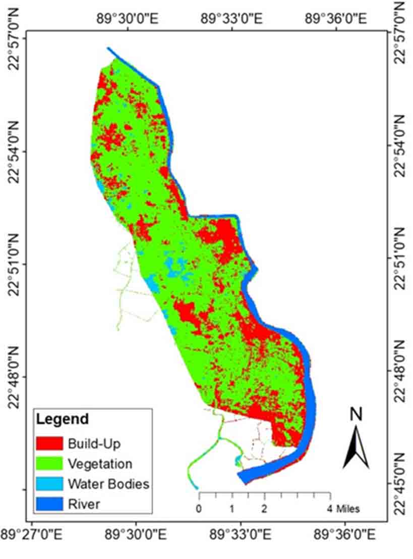
The confusion matrix was used to determine the precision of land use. The overall accuracy of the land use in the years 1987, 1996, 2007 and 2018 was 86%, 83%, 81%, and 82% (Table 4). As a dynamic area, the land use pattern of Khulna City Conurbation is changing continuously. Therefore, determining the accuracy of ancient satellite photos is challenging. The most recent land use classification in 2018 was based on a comprehensive ground-based analysis (Figure 6). For this study’s purposes, 50 spots across the study area were chosen at random for ground-truthing. The results revealed that of the 50 sites sampled, 44 sites corresponded to the 2018 land use map with an accuracy of 88%.

Figure 6. Ground truthing location

3.2 Ecosystem Services Valuation

The ecosystem valuation in this study was determined by cross-referencing the four land uses against the biomes proposed by Costanza et al. (1997) in their valuation methodology. Here, the ‘cropland’ biome was used for vegetation; the ‘wetland’ biome was used for water bodies; the ‘river or lake’ biome was used for rivers, and the ‘urban’ for built-up area. Equation 1 was applied to identify individual ecosystem services derived from land use and associated ecosystem service value coefficient. To calculate the ecosystem service value, the ecosystem service value was calculated by multiplying the ecosystem service value by the surface area of the current land use categories derived from the land use analysis using ArcGIS.

The values of ecosystem services in the Khulna conurbation were calculated by applying the value coefficient and area of land purpose types for 1987, 1996 and 2007, as well as for 2018. The total ecosystem value for existing land use of Khulna Conurbation in 1987 was 51.465 million US$, 53.40 million US$ in 1996, 56.97 million US$ in 2007, and 57.74 million US$ in 2018. From 1987 to 2018, the ecosystem service values for all land use categories were negative except for urban built-up. The largest amount of decline was observed in the case of vegetation which was about 11.79 million US$.

3.3 Ecosystem Services Sensitivity Analysis

Table 6 shows the change in total estimated ecosystem services and coefficient of sensitivity (CS) after modifying the ecosystem services valuation coefficient. The predicted coefficient of sensitivity for all land use categories was less than unity in all years. In terms of value coefficients, the projected overall ecosystem service values for the study region are mainly inelastic. Thereafter modifying the value coefficient by 50%, the coefficient of sensitivity value ranged from a lower 0.003 to 0.017 for water bodies to a higher 0.174 to 0.501 for built-up areas. This also confirms the robustness of the estimates for ecosystem service values.

4 . DISCUSSION

5 . CONCLUSION

The purpose of this paper is to analyse the effects of land use shifts on ecosystem services in the Khulna Conurbation. In the past three decades, Khulna City has seen a significant shift in its land use due to the rapid growth in population and the intensification of development. Changes in land use patterns have influenced overall ecosystem services. An increase in settlement area is a major threat as the conversion of land from agriculture and wetland into urban area led to a decreased ecosystem.

Since this study focused on inspecting the four types and their effects on ecosystem values, it is possible that the results may be different if more land types are used. Besides, there were fewer studies of ecosystem services and valuation in Khulna Conurbation, so there is a great opportunity to conduct more studies of the nearby regions and make a comparison among the regions. The value of urban ecosystem services has several implications for feasible land zoning planning due to its enormous influence on the well-being of urban dwellers. Urban vegetation, for example, regulates the urban heat island effect. Land conversion from vegetation to built-up can raise the power needed for air conditioning and warming buildings, escalating the number of public suffering from gasping ailments, and have a variety of other consequences.  The findings would be used to create a model to guide future land use decisions by identifying declining land types and ecosystem services that need more attention. The result would also be helpful for decision-makers and policymakers as they should consider the development of old Khulna city as lesson learning and should consider different urban planning techniques and principles for the further development of the city and enforce various environmental and ecosystem conservation measures to improve ecosystem services.

Tables

Figures

Conflict of Interest

Acknowledgements

Abbreviations

References