Keywords

Artificial neural network , Landslide Inventory , Natural hazard , Susceptibility Modeling

1 . INTRODUCTION

A single landslide is a substantial geological hazard that can cause significant property loss, numerous fatalities, and catastrophic damage to both natural ecosystems and man-made infrastructure (Ayenew and Barbieri, 2005; Hamza and Raghuvanshi, 2016; Apennine et al., 2019). Understanding the potential exposure to landslide hazards in mountainous and hilly terrain is necessary. Commonly, it is a downward mass soil or rock movement controlled by internal and external factors such as gravity, geology, presence of water, and morphology (Getachew and Meten, 2021; Wubalem, 2021; Mekonnen et al., 2022). Extreme natural disasters can result in infrastructure breakdown, property damage, and fatalities (Martnek et al., 2021; Shano et al., 2021). It is particularly severe in areas with rugged topography and diverse climatic conditions, such as the Alpine-Himalayan mountain tectonic belt (Petley 2012; Froude and Petley, 2018), the Ethiopian northern, southern, and western highlands, and areas near rift margins (Mengistu et al., 2019; Shano et al., 2021; Wubalem, 2021). Therefore, it is essential to assess and prevent landslides in this area.

In recent times, various models for landslide susceptibility mapping have been suggested. It is assumed that these models can evaluate landslide susceptibility by understanding the relationship between causative factors and susceptibility (Catani, 2004; Fall et al., 2006; Guzzetti et al., 1999; Hamza and Raghuvanshi, 2016). Landslide studies such as landslide susceptibility assessments and slope instability monitoring are important tools for disaster management and development activities. Given the appropriate geo-environmental parameters, landslide susceptibility is the possibility of slope failure (Shano et al., 2021). Owing to the complex and nonlinear nature of landslides, various methods have been developed and applied to landslide susceptibility mapping. These methods can generally be qualitative, bivariate, or parametric multivariate statistical methods (Cherie and Ayele, 2021; Getachew and Meten, 2021; Meten, 2020; Shano et al., 2021; Wubalem, 2021).

Although many models and techniques have been developed to produce Landslide Susceptibility Maps (LSM) (Apennine et al., 2019; Froude and Petley, 2018; Petley, 2012), due to their lower subjectivity and simplicity, statistical methods are the most popular in landslide susceptibility modeling. Among statistical methods, both bivariate and multivariate approaches have been widely used in many susceptibility analyses. Using bivariate statistical methods (Senise et al., 2013; Won, 2003), the contribution of each landslide-inducing factor to slope failure susceptibility was evaluated individually, overlooking the possibility that the different aspects may have a mutual relationship. Compared with traditional methods, landslide susceptibility mapping is becoming more optimized, automated, and simple because of advancements in processing power and remote sensing, more sophisticated Machine Learning (ML) methodologies, and high-resolution optical and active remote sensing imageries. In studies on landslide susceptibility modeling, ML methods have proven promising because they can comprehend and model complicated and nonlinearly connected situations (Westen et al., 2008; Zêzere et al., 2017; Mohamed and Reza, 2021; Yang et al., 2020). Artificial Neural Networks (ANN) are data-driven methods that circumvent most of the aforementioned restrictions. This model can process data and learn sophisticated model functions by ‘training’ using input and output data (Bragagnolo et al., 2020; Lee et al., 2004; Melchiorre et al., 2008). For landslide susceptibility modeling, more recent publications have highlighted multivariate logistic regression methods (Bui et al., 2015), knowledge-based methods (Kumar and Anbalagan, 2016), Random Forest (RF) (Mohamed and Reza, 2021), maximum entropy-MaxEnt, Support Vector Machine (SVM), and logistic regression (Chen et al., 2018; Lin et al., 2017).

Previously, numerous studies have investigated landslide susceptibility as a spatial distribution of the probability of landslide occurrence (Wubalem, 2021; Mekonnen et al., 2022). Landslide monitoring, inventory updates, and fieldwork optimization have recently become more accessible because of the advent of high-resolution sensors, such as SPOT, IKONOS, Worldview, Google Earth, Sentinel-1 (TerraSAR-X or Cosmo-SkyMed), and Sentinel-2. Given its ability to track the occurrence or reoccurrence of landslides day and night regardless of weather conditions, Synthetic Aperture Radar (SAR) remote sensing is a potentially ideal solution for detecting and mapping landslides (Cherie and Ayele, 2021; Mengistu et al., 2019). Geographic Information Systems (GIS) technology can help construct landslide susceptibility zones determined by the synergistic effects of several regional geological and environmental elements. Our findings have the potential to significantly contribute to the scientific community. The significance and novelty of this research lie in its pioneering effort to generate a comprehensive landslide susceptibility map in the selected road corridor area, making it an effective landslide risk management strategies along the road corridor of the study locally. This study addresses the crucial need for accurate landslide susceptibility assessment in a region characterized by complex topography, where landslides pose significant hazards to communities and infrastructure. The novelty of this study stems from the integration of various datasets, including landslide inventory maps, topographic factors, and environmental variables, as well as the application of the ANN model. Therefore, a study was conducted to compare and contrast the use of ANN to optimize the causal factors in assessing landslide vulnerability in the Sawla-Laska road corridor and neighboring areas of southwest Ethiopia. The findings of this study can be highly beneficial for strategies to reduce the risk of landslides, land use planning, and regional development initiatives.

2 . MATERIAL AND METHODS

3.1 Study Area

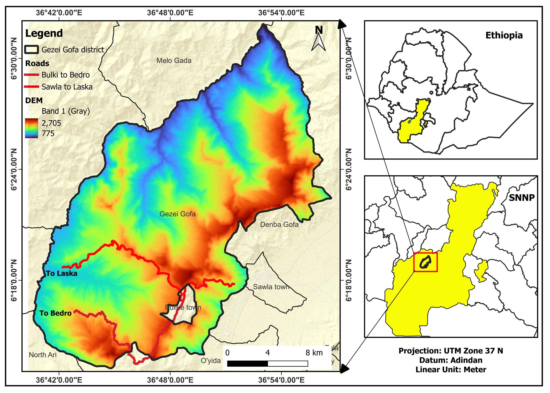
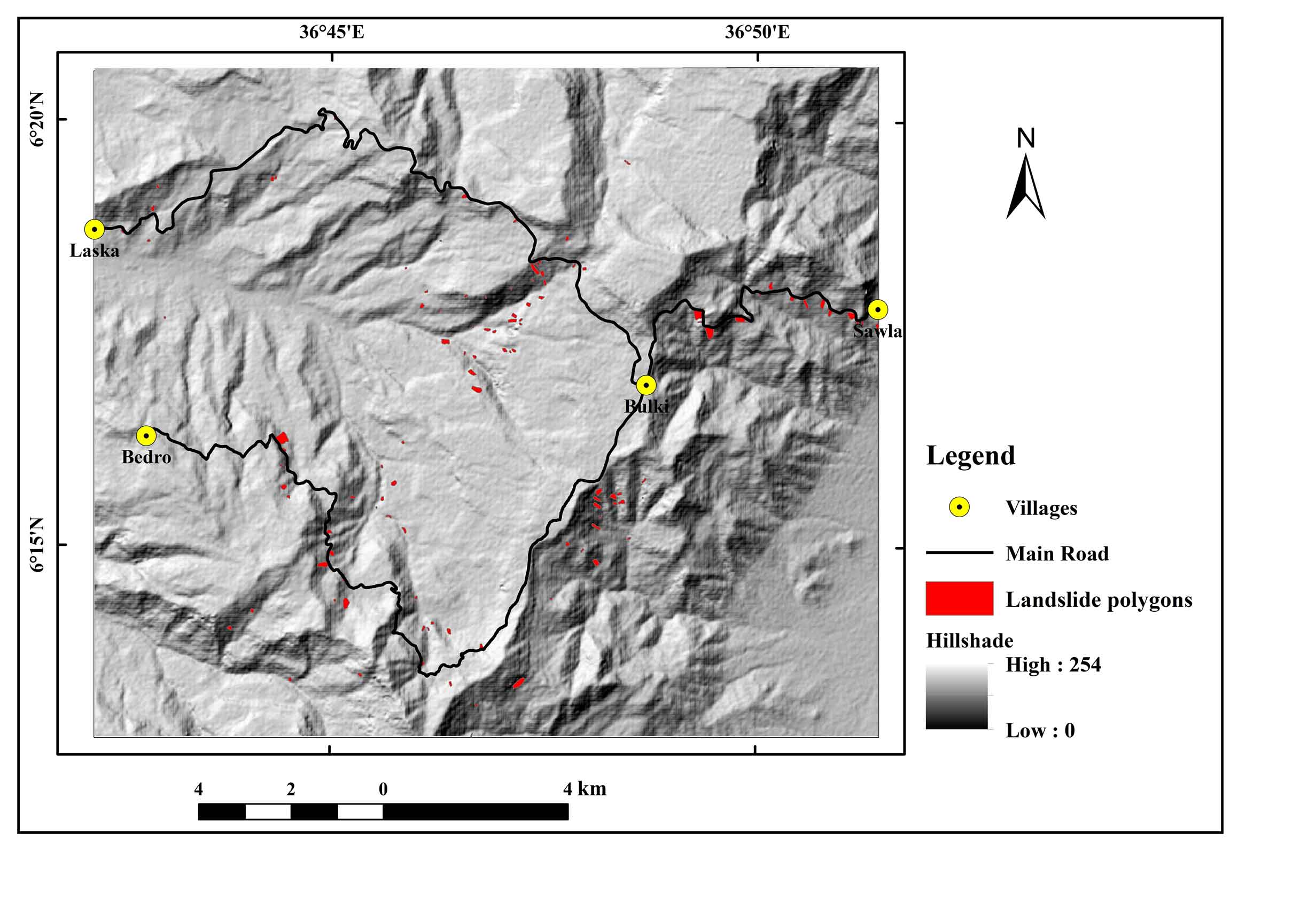
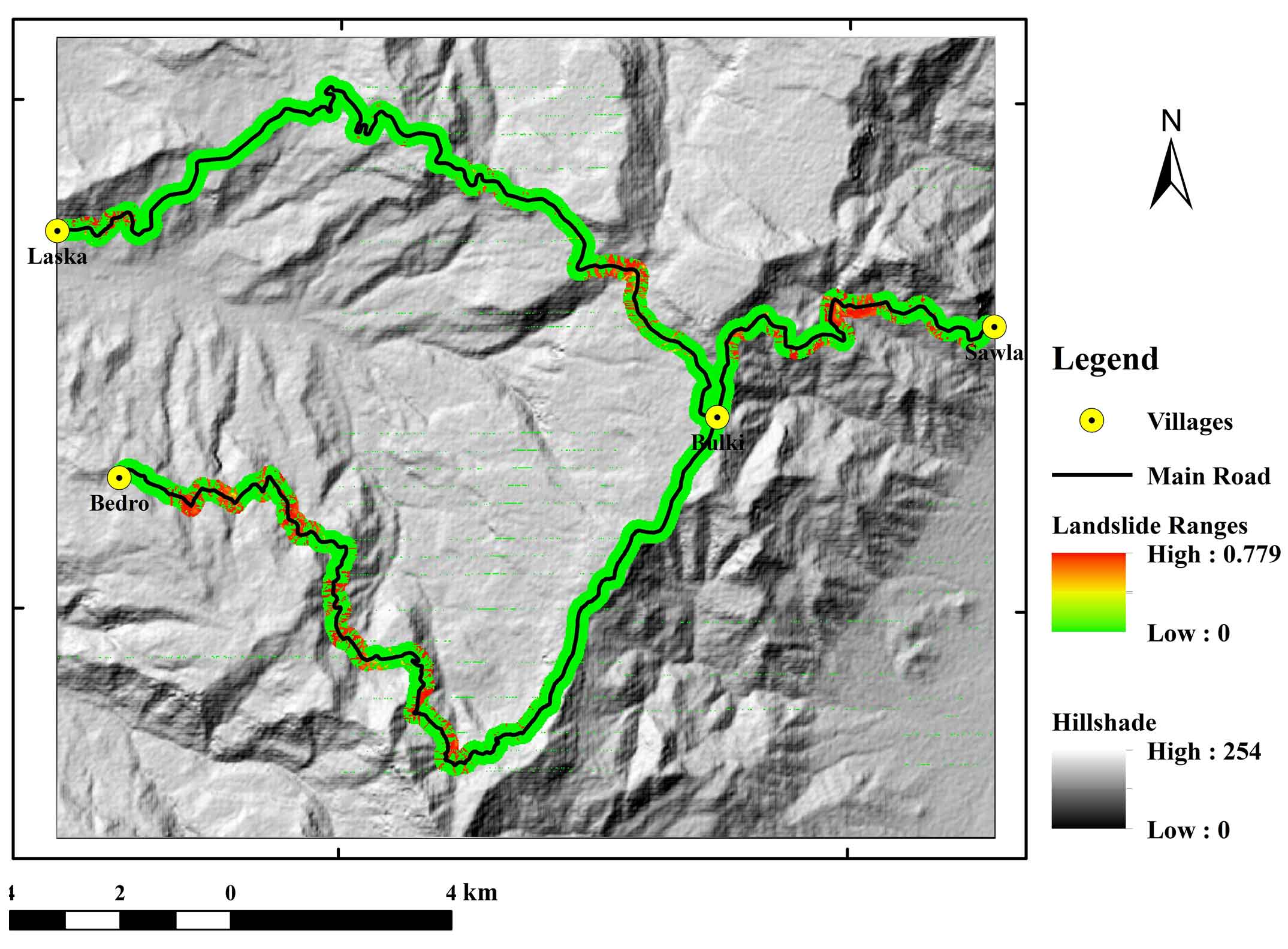
This investigation was carried out in the Semen Omo Zone, within the Geze Gofa District, in southwest Ethiopia, along the key roads connecting Bulki to Laska and Bulki to Bedro (SNNP). The area is accessed from the capital of Addis Ababa by traveling to Wolayita Sodo, Sawla town, and the Bulki-Laska routes. Geographically, it lies between 36^o43′0″-36^o52′0″ longitude and 6^o13′0″–6^o20′0″ latitude, covering a total area of 246 km² (Figure 1). The region on the western edge of the major Ethiopian Rift Valley is notable for its complex and rocky landscape. It is a portion of the southern Ethiopian Plateau, and the Rift Valley borders it to the west. Over the study region, the elevation varies significantly, reaching a maximum of almost 2600m (in northern Bulki) and a minimum of 1200m (on the Irgina course). Surface water and groundwater are plentiful resources in the study region because of the area’s considerable rainfall (an average of 1347mm per year). The main rivers are the Irigine and Meto from which several smaller rivers flow.

Figure 1. Study area

3.2 Regional Geology

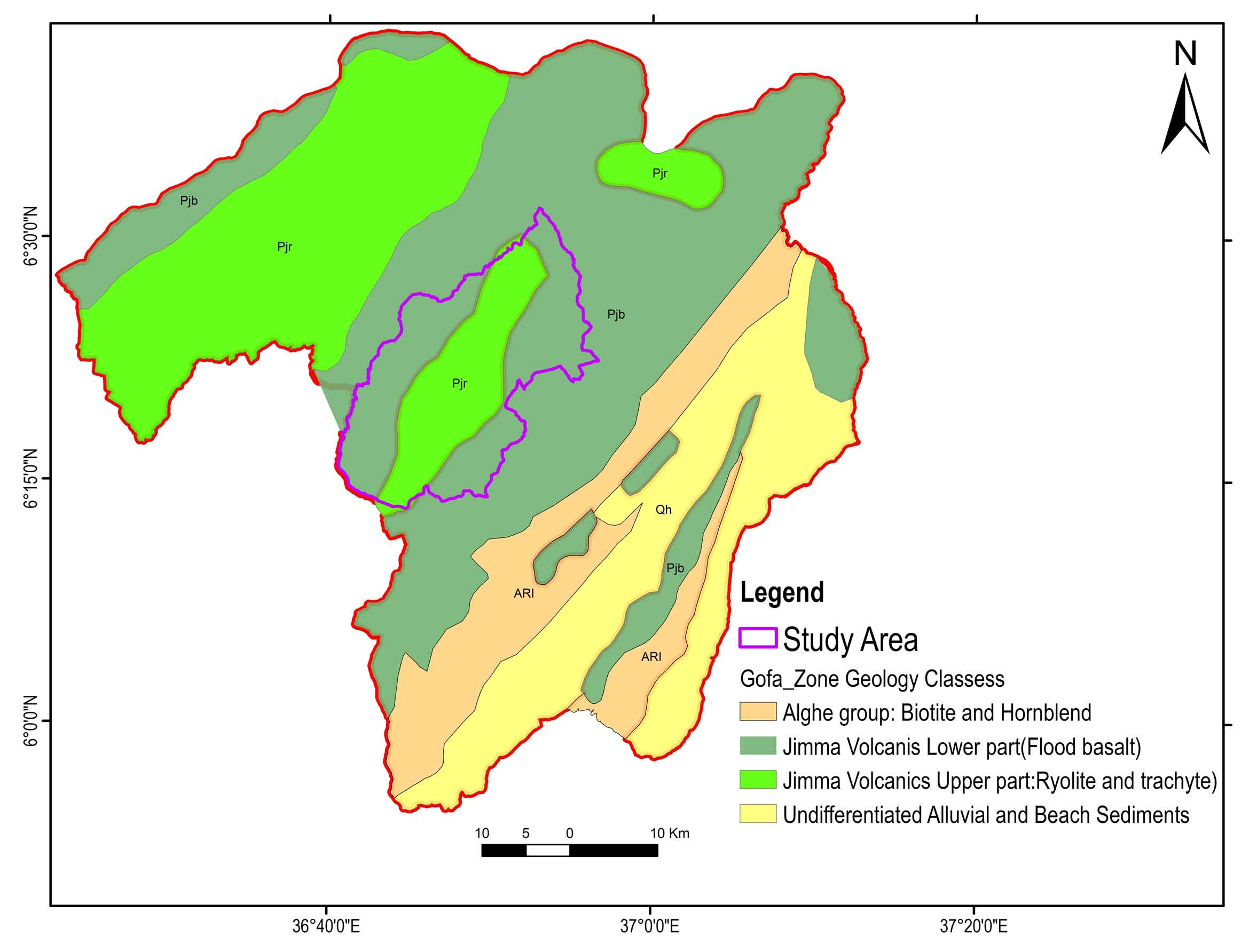
The frequency of landslides in a region is primarily influenced by its geology. The region’s geological structure is supported by Tertiary volcanic rocks, quaternary alluvial sediments, and other volcanic flows and pre-rift and post-rift successions make up the Cenozoic rocks in southwest Ethiopia. Southwest Ethiopian Cenozoic rocks are divided into pre and post-rift successions (Haregot et al., 2017). The geology of the majority of the study area is composed of pre and post-rift deposits. Holocene sediment deposits are found in post-rift, Early Flood Basalts, Salic, Basaltic, and intermediate flows, and pyroclastic rocks are among the pre-rift deposits (Haregot et al., 2017). Massive lava flows that characterize the Jima basalts, which have grown to a height of more than 2400m, comprise the majority of the geology along road corridors and in other locations. Along road sections, colluvial deposits containing silt, clay, and gravel are widely scattered. They are composed of varying-sized rock elements (cobbles and boulders). The upper portions of the geological strata are covered by such materials, which are transported by gravity from the higher ground. Owing to their larger grain sizes and widespread distribution along road corridors, these formations are both poorly sorted and highly porous. Colluvial deposits are particularly prone to landslides because they primarily lose their shear strength when they occupy steeply dipping topographies and become saturated. Additionally, the study area exhibits significant structural deformation, as evidenced by the presence of numerous faults, folds and joints (Figure 2).

Figure 2. Geology

2.3 Data and Software

In this study, freely accessible satellite data and additional auxiliary datasets were obtained for this investigation. Sentinel-2A, ALOS PALSAR DEM, Google map satellite datasets, topography, GPS, and soil data were utilized. The remote sensing data collected for this study are shown in Table 1. The remote sensing and GIS software were used in this study included QGIS 2.18 for creating model training and testing datasets, ArcGIS 10.3 for creating thematic layers for landslide causative factors, Google Earth Pro for extracting landslide scars, and RStudio 1.1.463 for creating ANN models to model landslide susceptibility final output throughout the entire study (Arnone et al., 2016; Pham et al., 2017; Pourghasemi and Rahmati, 2018).

3.3 Methodological Approach

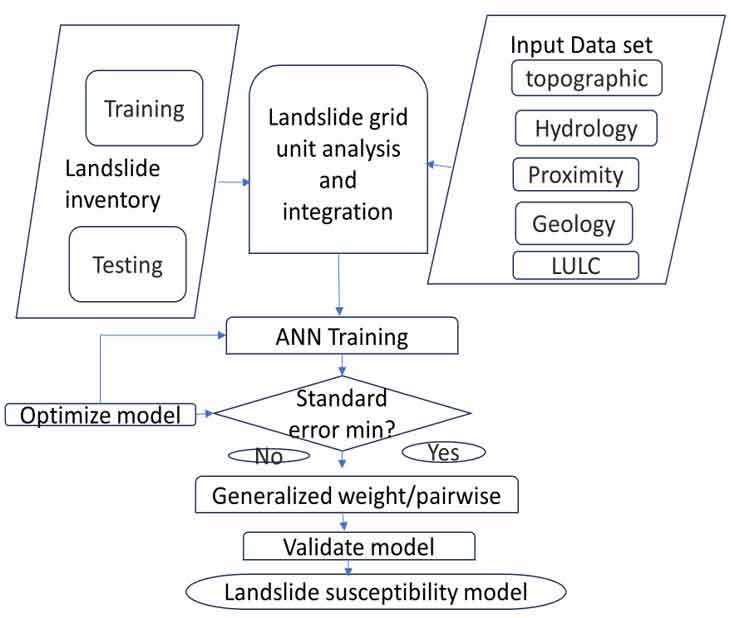
This study aims to map the spatial components of landslide susceptibility. Input data gathering, mapping of landslide inventories and causal factors, extraction of training and testing datasets, model training, and model validation and prediction stages comprised the five main components of the ANN approach used in this study. The overall methodology of this study is presented in a flowchart (Figure 3).

Figure 3. Conceptual diagram of an application of ANN model for landslide susceptibility map

3.3.1 Landslide Inventory map

Creating a reliable inventory map is a crucial first step in determining landslide susceptibility (Hamza and Raghuvanshi, 2016; Mengistu et al., 2019; Shano et al., 2021). Making a landslide inventory is the initial stage in ANN-based landslide susceptibility analysis, which is used to train and test the model. Accordingly, 195 landslide polygons were collected for this research based on prior landslide data, field survey examination, and Google Earth scars. According to area statistics, the least, mean, and maximum landslide polygons cover 406 m², 6995.7 m² and 657004 m² of space, respectively. The majority of the slides in the inventories were gathered along the road corridors that cut across the steep terrain. In addition, numerous landslides from various locations in the research area were collected after the landslide event that occurred on September 11, 2021 (Figure 4).

Figure 4. Existing landslides

3.3.2 Landslide Causative Factors

Input datasets with thematic focus must be prepared for landslide susceptibility analysis. Numerous theme categories, including topographic, hydrologic, geological, proximity, environmental, and triggering elements, have been used to identify different landslide-deriving factors based on prior studies and study region conditions.

3.2 Topographic Factors

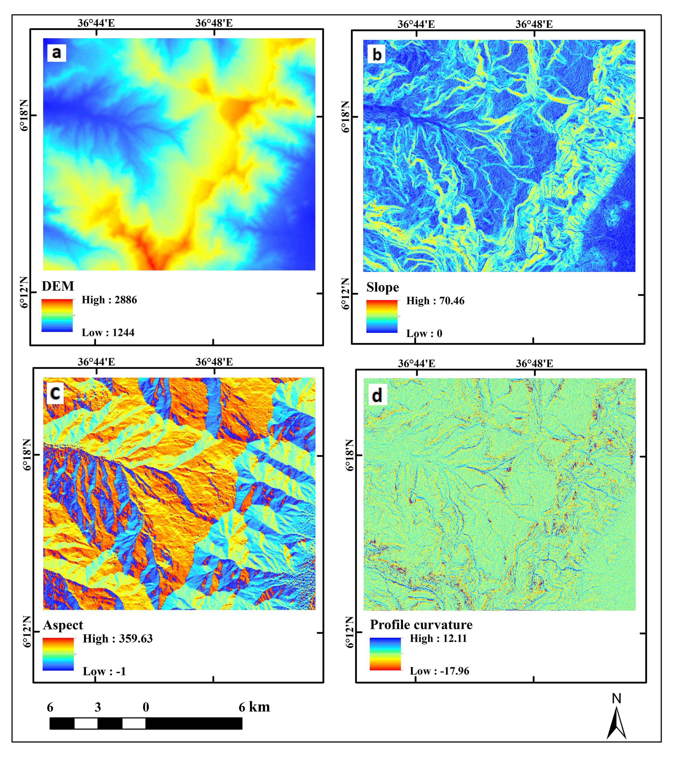
The most significant variable influencing the likelihood of landslides was geomorphology. The basic Digital Elevation Model (DEM) of the current study was derived from the slope, aspect, plan curvature, and profile curvature, which are crucial for preventing landslides. Due to the fact that landslides are inextricably linked to slope perspectives, the slope is frequently used in landslide susceptibility assessments. According to Shano et al. (2021), this is the only significant factor that directly affects soil water content, formation, erosion potential, and slope stability. Because weather and climate change depend significantly on elevation, altitude is a significant contributor to the occurrence of landslides. Changing the amount of rainfall and vegetation cover indirectly affects the slope instability (Mohamed and Reza, 2021). Because weather and climate change depend significantly on elevation, altitude is a significant contributor to the occurrence of landslides. Changing the amount of rainfall and vegetation cover indirectly affects the slope instability (Mohamed and Reza, 2021). Aspects have also been considered a landslide-controlling component in numerous studies. Lowering the ability of sunlight to heat the earth efficiently affects the moisture content of the soil and represents the direction of the slope face (0°-360°). Another crucial DEM derivative for landslide occurrence is the plane and profile curvature. They demonstrated the impact of terrain morphology and slope form on the landslide susceptibility mechanisms. This affects erosion by causing water flowing downhill to converge or diverge (Senise et al., 2013). A positive plan curvature indicates convexity, zero curvature indicates flatness, and negative curvature indicates concavity. The profile curvature governs the change in the velocity of the mass flowing down a slope and displays the flow expedition, erosion rate (negative values), and deposition (positive values) rates. This was the curvature of the corresponding standard section. All topographic derivate were created using the 12.5m resolution ALOS DEM (Figure 5).

Figure 5. DEM (a), Slope (b), Aspect (c) and Profile curvature (d)

3.3 Hydrological Factors

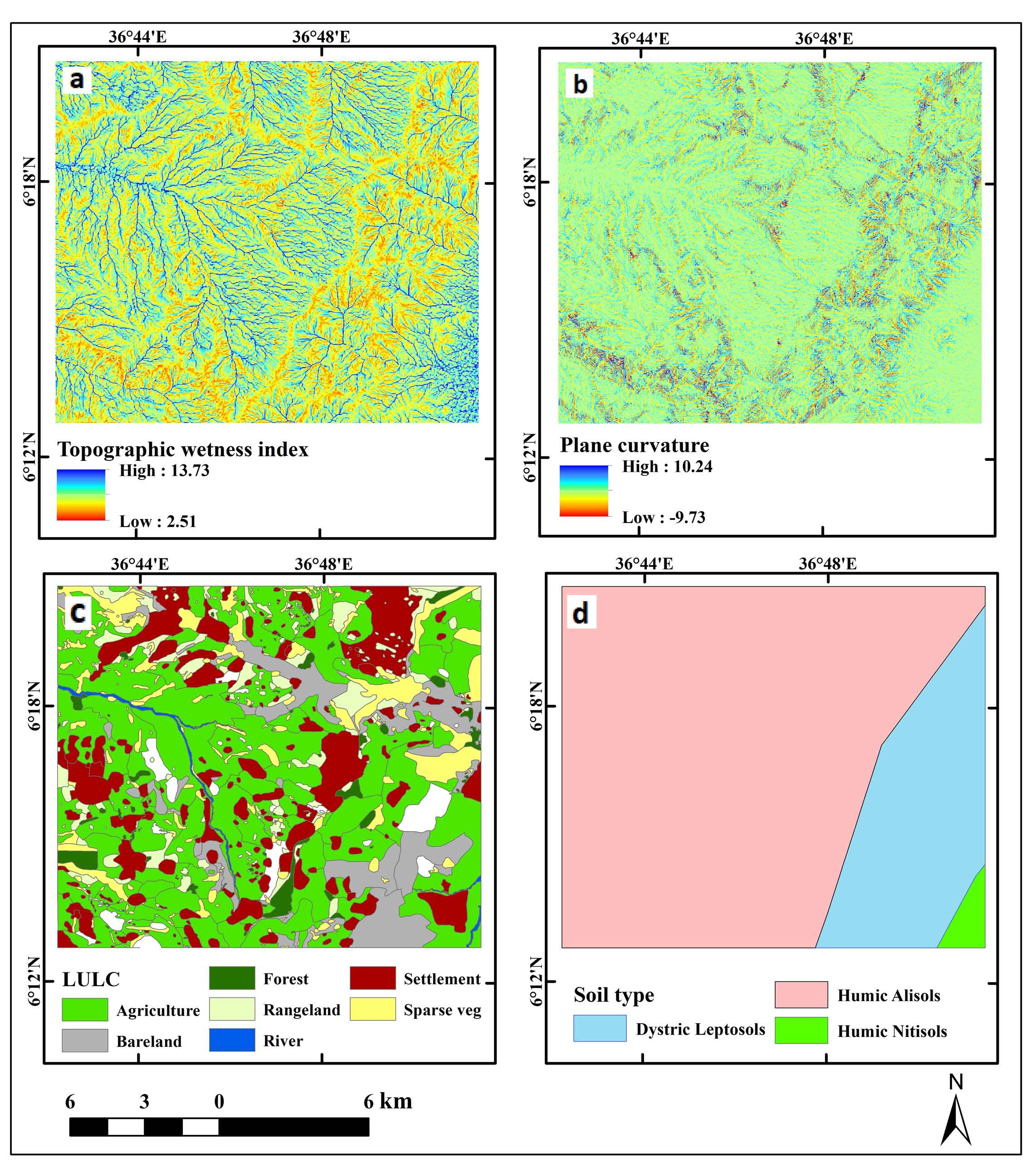
Landslides are frequently caused by hydrological factors. The hydrological elements that affect landslides include drainage density, groundwater, and precipitation distribution. The Topographic Wetness Index (TWI) is one of the most frequently used landslides. However, due to a lack of data, research on landslides has only occasionally included information about groundwater. Secondary DEM derivatives that make it easier for landslides to occur include the drainage density and TWI. Landslides tend to occur along drainages because erosion and excavation near rivers can build up the requisite potential energy for landslides to occur. Consequently, landslide susceptibility can be calculated as a function of the relationship between topographic influences and a region’s hydrological response (Althuwaynee et al., 2012; Chen et al., 2018). It provides information on groundwater movement, accumulation, and soil moisture conditions. The slope grade and catchment area can be used for the computation. The TWI was determined by applying Eq. (1), which is based on the steady-state hypothesis for uniform soil conditions:

​\(TWI= In { {(\alpha) \over (tan \beta) }} \)​                         (1)                                                                                                                                         

where ​\(\alpha\)​ and ​\(\beta\)​ is the cumulative upslope and the slope angle at the point, respectively.

3.4 Geological Factors

The geological composition of the study area plays a critical role in landslide susceptibility mapping. Lithological variations have a significant impact on different types of geo-hazards (e.g., such as landslides and land subsidence) (Mekonnen et al., 2022). These units vary in physical and mechanical characteristics, including the type and strength, degree of weathering, durability, density, and permeability (Shano et al., 2021). In addition to lithology and geological structures such as faults, lineaments, and fractures, geological variables such as faults and lineaments also play a significant role in landslide conditioning. Diverse soil types play various roles in determining landslide vulnerability, depending on factors such as the texture and erodibility index. According to Cherie and Ayele (2021), soil erodibility index values have a linear effect on the likelihood of landslides. From the EthioGIS soil database, three different soil types, Humicalisol, Humicnitosol, and DystricLeptosol, were extracted for this investigation. The corresponding values for erodibility and texture types were loam (0.12330), loam (0.1273), and sandy loam (0.15).

3.5 Anthropogenic Factors (Environmental)

Anthropogenic factors include environmental influences caused by humans and other living organisms. Anthropogenic components, including poor land-use planning, are one of the conditioning variables contributing to slope stability (Mekonnen et al., 2022). The manner in which land is used and covered significantly affects landslides. Although regions with adequate vegetation cover tend to be more stable, inappropriate land management practices can cause slope instability. Unplanned agricultural operations are growing drastically in the study area’s steep terrain and road corridors. Sentinel 2A images and a real-time Google satellite map were used to extract an alternative land-cover map for the study area (Figure 6). Google satellite maps have obtained satisfactory results and excellent for extracting training and testing datasets because they are high-resolution satellite photos that users can manage (Mersha and Meten, 2020; Meten, 2020; Shano et al., 2021; Wubalem, 2021). Seven land-cover categories, including agriculture, settlements, sparse vegetation, forests, rangeland, rivers, and barren areas, were subsequently extracted. Incidences of landslides are also significantly influenced by the Normalized Difference Vegetation Index (NDVI). According to Mohammed and Reza (2021), the NDVI can improve the lithological mass’s soil cohesiveness and shear resistance. Using the QGIS framework and a plug-in for semi-automatic classification, NDVI was calculated using sentinel 2A imagery.  Due to their capacity for green reflectance on that wavelength spectrum, the sentinel 2 bands’ spectral values in the red band and near-infrared were used for this purpose (Kebede et al., 2022). It was extracted using Eq. (2).

​\(NDVI = {B_{nir} - B_{red} \over B_{nir}-B_{red }}\)​          (2)          

Figure 6. Topographic wetness index map (a), Plane curvature (b), LULC (c) and Soil map (d)

3.6 Proximity Factors

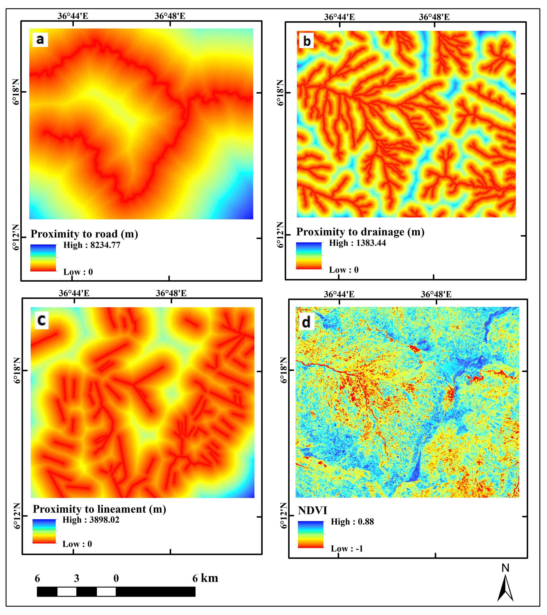
Distances to highways, faults, and rivers can be used to estimate these geographic features related to environmental fragility and human development. In different situations, these elements may affect the likelihood of a landslide. Following building excavations and human activity, landslides frequently happen along road corridors. Another nearby element that affects landslide susceptibility is drainage density. As the distance from streams reduces and erosion and water transportation activities increase, the area becomes more vulnerable to landslides (Figure 7).

Figure 7. Proximity to road (a), Proximity to drainage (b), Proximity to lineament (c), and NDVI (d)

3 . DATA ANALYSIS OF ANN

This stage involved rasterizing all thematic layers that were in vector format, resampling them to a common pixel size of 20m, and projecting them to the UTM 37N zone. The ANN-based landslide susceptibility analysis consists of a grid unit analysis of the landslide, training of the ANN model, model performance validation, and susceptibility prediction. The ANN is a quantitative method that makes use of nonlinear and complex learning and prediction algorithms to extract the complex relationships among the various independent landslide variables. The purpose of an ANN is to build a model of the data-generating process, so that the network can generalize and predict outputs from inputs that it has not previously seen. In the current analysis, the “rminer” package (Cortez, 2020) was used for carrying ANN model by 12-6-1 network and learning rate of 0.1.

4.1 Extracting Training and Testing of Landslide Grid Units

Landslide inventory and thematic raster layers of landslide conditioning variables are two fundamental datasets for preparing training and testing datasets. The landslide inventory dataset was split into training and testing datasets for this purpose, with 80% (156) and 20% (39) of each dataset used for training and testing model performance, respectively. For landslide susceptibility analysis, landslide conditioning factors are a crucial data collection in addition to landslide events. As a result, landslide grid cells were created by intersecting 12 thematic conditioning factors with landslide polygons. In order to develop the model, a total of 1482 binary points were retrieved, of which 225 landslide zones and 1257 representing non-landslide areas were extracted for the model’s construction. Similarly, based on landslide grid unit analysis in the QGIS environment, 448 non-landslide (zero) and 65 slide pixels were recovered from the 39 testing datasets.

4.2 Training Artificial Neural Network Model

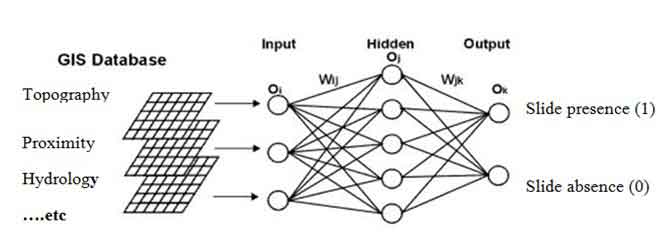
Extracted training and testing data sets with independent and dependent inputs were used to train the Artificial Neural Network (ANN). Input-hidden-output layers make up the input-hidden-output configuration of an ANN, as depicted in (Figure 8). The output layer represents the landslide training datasets (presence and absence), while the input layer represents the landslide causative raster datasets. The hidden layer reflects internal processing operations. When landslides are present or absent, represented in binary form as 1 and 0, respectively, the model is trained to identify grid unit pixels. The training datasets must be of a numeric data type and scaled to a range between 0 and 1 in order to be used to train the model. As a result, all inputs were standardized between 0 and 1 in the R software environment and nominal (categorical) training inputs such as land-cover, aspect, and soil were converted to numeric data format. The seven land cover classifications were given the numerals 10, 11, 12, 13, 14, 15, and 16 for agricultural, settlement, sparse vegetation, forest, range land, river, and barren land, respectively. The aspect classes were further divided into eight categories, with letters ‘a’, ‘b’, ‘c’, ‘d’, ‘e’, ‘f’, 'g', and 'h' allocated for the aspect ranges 0^o-45^o, 45^o-90^o, 90^o-135^o, 135^o-180^o, 180^o-125^o, 125^o-270^o, 270^o-315^o and 315^o-360^o, respectively. For Dystric Leptosols, Humic Alisols, and Humic Nitisols, respectively, the initials M, N, and P were used to designate the three soil classifications.

 

Figure 8. Modified Neural Network model structure (Lee et al., 2004)

 

Weight Determination Strategies

The inputs are multiplied by the appropriate weights in the hidden and output layer neurons, the product is added, and the sum is then processed using a non-linear transfer function to provide a result (Lee et al., 2004). Synaptic weights, or ​\( w_{ij} \)​ , between neurons I and j determine the connections between the neurons. The weights are computed by ANN using an assessment of the error between the propagation response and the known true value of the output. Finally, the model was trained using four different input-hidden layer-output structure techniques based on Eq. (3). The model was trained using a 12-2-2 or 26-2-2 network structure with default weight settings (including categorical classless for aspect, soil, and land cover). The second, third, and fourth training phases of the ANN were simultaneously learned using the 12-5-2, 12-10-2, and 11-15-2 or 26-5-2, 16-10-2, and 16-15-2 containing categorical classes, respectively.

​\(net_{j} = \sum_{i}^{n} w_{ij} \times o_i\)​          (3)                                                                                                                             

where ​\( w_{ij} \)​  represents the weight between node i and node j, and ​\( o_{i} \)​  is the output from node i.

After the synaptic weights have been given to the neurons, an activation function is used to keep the amplitude of each neuron’s output value between 1 and 1 (Neaupane and Achet, 2004). According to Eq. (4), the S-shaped sigmoid function is a transfer function with a balance of linear and nonlinear behavior.

​\(f(x)= { {1 \over 1+e^{-x} }} \)​                     (4)                                                                                                                                      

where x represents weight summation at hidden layers.

In order to train an ANN, it must first go through a process known as back propagation, which involves calculating the weight values by comparing the response obtained through propagation to the output’s known real value. By altering synaptic weights during training, the back propagation technique seeks to reduce error function E. Therefore, the reference output (Lee et al., 2004), Ok, and the corresponding output (k) for each example provided during training are contrasted, resulting in the error function illustrated in Eq. (5).

​\(E = {1 \over 2} \sum_{k} (p_k-o_k)^2\)​            (5)                                                                                                             

where ​\(p_{k} \)​ and ​\( o_{k} \)​ is represent predicted output and observed output, respectively.

4.3 Model Optimization

Selecting landslide conditioning factors is a crucial step since some noisy parameters may reduce the LS forecasting ability of the model (Lee et al., 2004). Therefore, it is necessary to determine the impact of landslide-deriving factors on the occurrence of landslides before selecting a final landslide susceptibility model structure. The internal learning capacity of the model was increased, and some inputs were filtered using generalized weight and pairwise analysis. Some factors were discovered to be less predictive during the first and second training phases and were removed from the final model analysis.  The model was trained using the hidden layers and highly predictive inputs. Because some noisy factors may decrease the LS forecasting performance of the model, selecting landslide conditioning factors is a key step (Lee et al., 2004). So, before choosing a final landslide susceptibility model structure, there is a need to identify the effect of landslide-deriving factors on landslide occurrence. The model performance was optimized by increasing internal learning capacity and filtering some inputs based on the generalized weight and pairwise analysis. Some factors were found to be less predictive during the first and second training phases and reduced from the final model analysis. Accordingly, the optimized model structure was again adjusted, consisting of 12-2-2, 12-5-2, 12-10-2, and 12-15-2 or 26-2-2, 16-5-2, 16-10-2, and 16-15-2 input-hidden-output NN structures.

4 . RESULTS

4.1 ANN Model

The training phase results are typically represented by error functions, which gauge how well the network fits the training set of observed data, such as the total squared error or cross-entropy error functions. Table 2 illustrates how several network architectures were used to apply the four learning phases. As a result, learning errors between observed and anticipated outputs were attained using the model structure with the optimum RMSE.

4.2 Generalized Weights (GW) of Factors

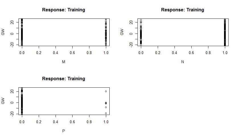
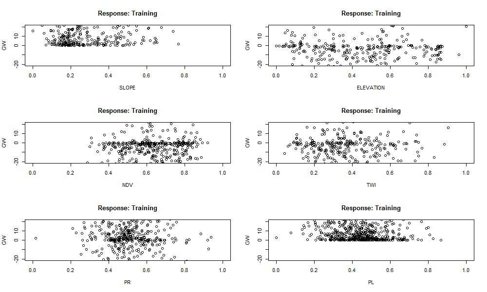
The neural network model’s first significant finding was the weighted link between landslide factors and the actual landslide. Based on the above preliminary network statistics, it was decided. Figure 9 shows the obtained generalized weight between the explanatory and response variables. Each plot has a horizontal distribution of the scaled input datasets and a vertical assignment of the corresponding weight ranges. The weight vs. input plots’ output reveals three distributions for the input datasets. Some input datasets are populated along zero-weight ranges, while others are spread along ranges above and below zero. In other words, there is a positive link between landslide and input variables and vice versa if the datasets are distributed above the zero weight.

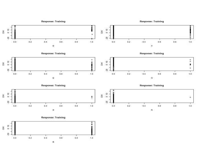
The landslide weight connection for each type of soil is depicted in (Figure 9). The findings show that the soil classes M (Dystric Leptosols), N (Humic Alisols), and the response variable (landslide) have a positive or significant association. The third soil class, on the other hand, has no or a weak link with the occurrence of landslides in the studied area. The GW association for six causal factors is also shown in (Figure 10). Results showed that every component is significant and can forecast landslide susceptibility. The findings showed a significant correlation between slope plane curvature and the likelihood of landslides. Elevation, TWI, and PR all showed positive and negative connections with one another. A high correlation was also found between the occurrence of landslides and the proximity factor (Figure 11). This is connected to human activity along drainage corridors, traffic corridors, and lineament faults. The GW values for different kinds of land cover are shown in (Figure 12). Results show that both positive and negative contributing factors to landslide incidence are found in the terrain classifications of agricultural (10), settlement (11), scant vegetation (12), and bare (16). That indicates that they attained weight values larger than zero, either below or above. The river (15), rangeland (14), and woodland (13), on the other hand, were unaffected by the landslide weight. As a result, since these characteristics were determined to have no bearing, they were eliminated from the prediction of landslide susceptibility.

Figure 9. Generalized weight for soil classes

Figure 10. Generalized weight for six causative factors

Figure 11. Generalized weight for proximity factors

Figure 12. Generalized weight for LULC classes

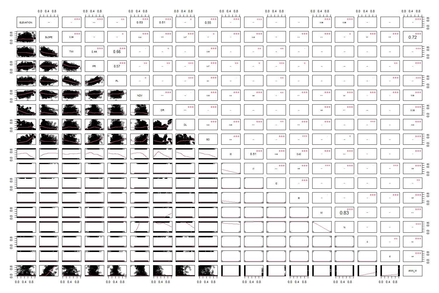
4.3 Generalized Weights Among Covariates (Landslide Causative Factors)

The large contribution of landslide-deriving factors (covariates) was also generated during generalized weight analysis. The output of the pair-wise matrix and important rank values are shown in (Figure 13). Landslide values (ranks) among the factors are represented in the last column on the right. The result showed that slope was the strongest controlling factor, with a very significant rank value of 0.72. Following slope proximity variables, the NDVI, agriculture, settlement, and barren land were also noted as the primary controlling elements. A diagonal line represents all the covariates, and the significant rankings between them are shown visually below and above. For instance, the correlation between settlement and agriculture (0.51), between TWI and PL (0.66), and between PR and PL (0.57) all attained significant scores, indicating a high likelihood of landslide derivation.

Figure 13. Generalized weight between covariates

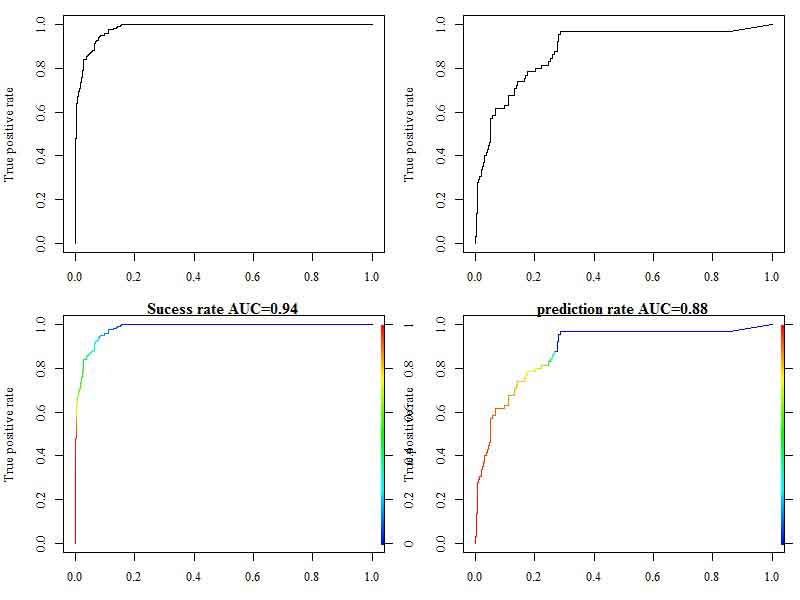
4.4 Model Validation

The receiver operating characteristic curve (ROC) curve and area under the curve (AUC) approaches were used to evaluate the model’s learning and prediction capabilities. The model’s learning performance was evaluated using 80% of the binary training datasets, while its prediction performance was evaluated using 20% of the testing datasets. ROC curves were used to determine the likelihood that the landslide and non-landslide cells would be accurately identified, as illustrated in Tables 3 and 4. In the ROC plot, the positive rate represents the likelihood that a landslide pixel is correctly placed and shown on the Y-axis. On the other hand, the likelihood that a non-landslide cell is correctly identified is known as the actual negative rate. The performance of the created model for forecasting landslide susceptibility was finally quantitatively quantified by AUC. Figure 14 shows training pixels (slides and non-slides) of ROC and AUC analysis findings, which may be used to assess the model’s performance. The training pixels summary shows that, out of the 1257 non-slide pixels, 1201 were correctly identified, and 65 were misclassified. Likewise, 175 of the 225 pixels from the landslide (1) were correctly classified, while only 50 were incorrectly labeled. The model quantitatively attained a 94% learning success rate. The findings of the ROC and AUC plots are shown on the right side of Figure 14 as testing pixels (slides and non-slides). The 385 pixels were successfully identified as non-slides according to the model testing pixels, while 63 pixels were incorrectly identified from 448 non-slides (0). Similarly, 15 slides were incorrectly classified as 0, whereas 50 were correctly classified as 1. The ROC and AUC guarantee that the model has a predictive performance of 88%, demonstrating that it can forecast landslide susceptibility across the entire study area.

Figure 14. ROC and AUC of the model learning and prediction rates

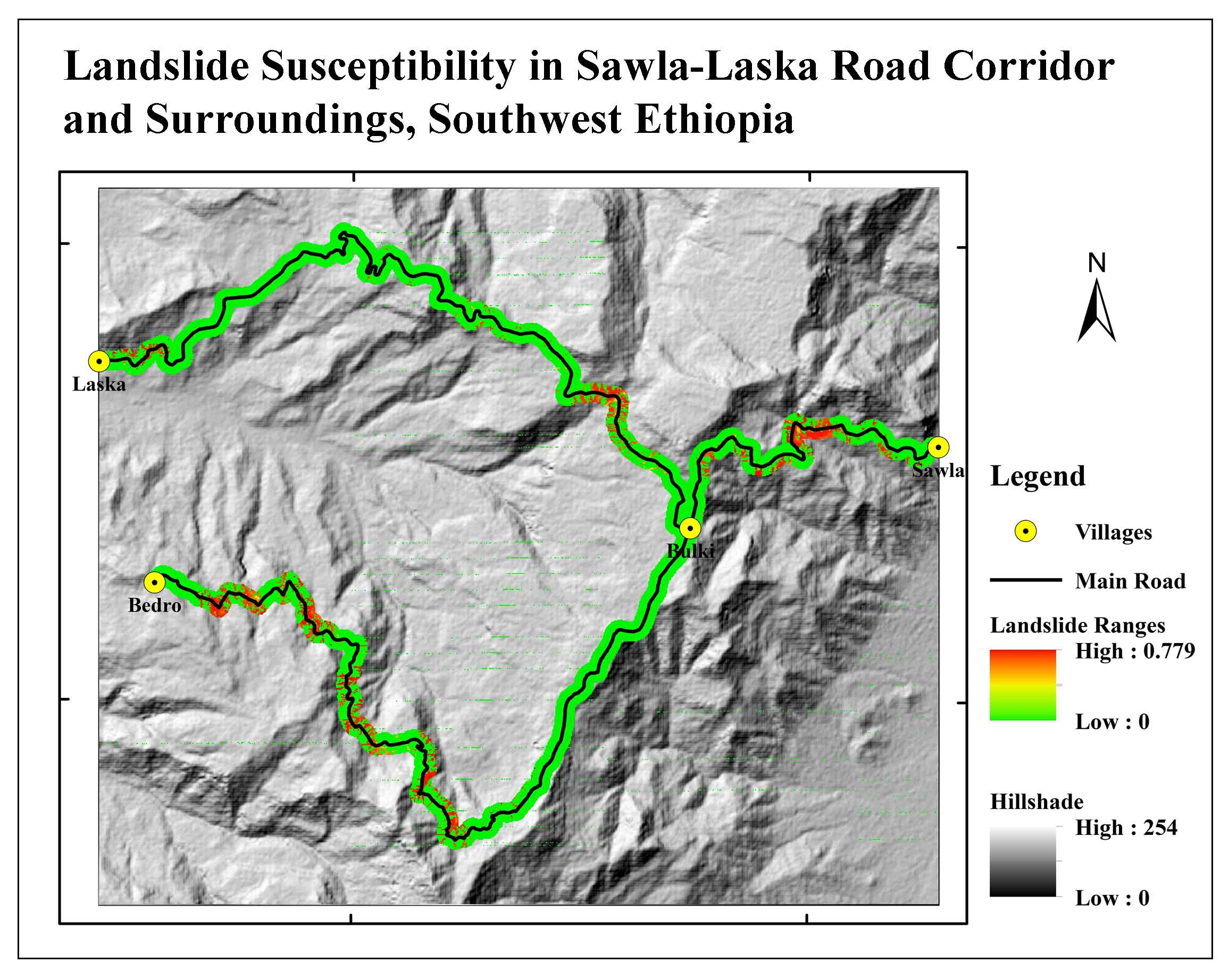
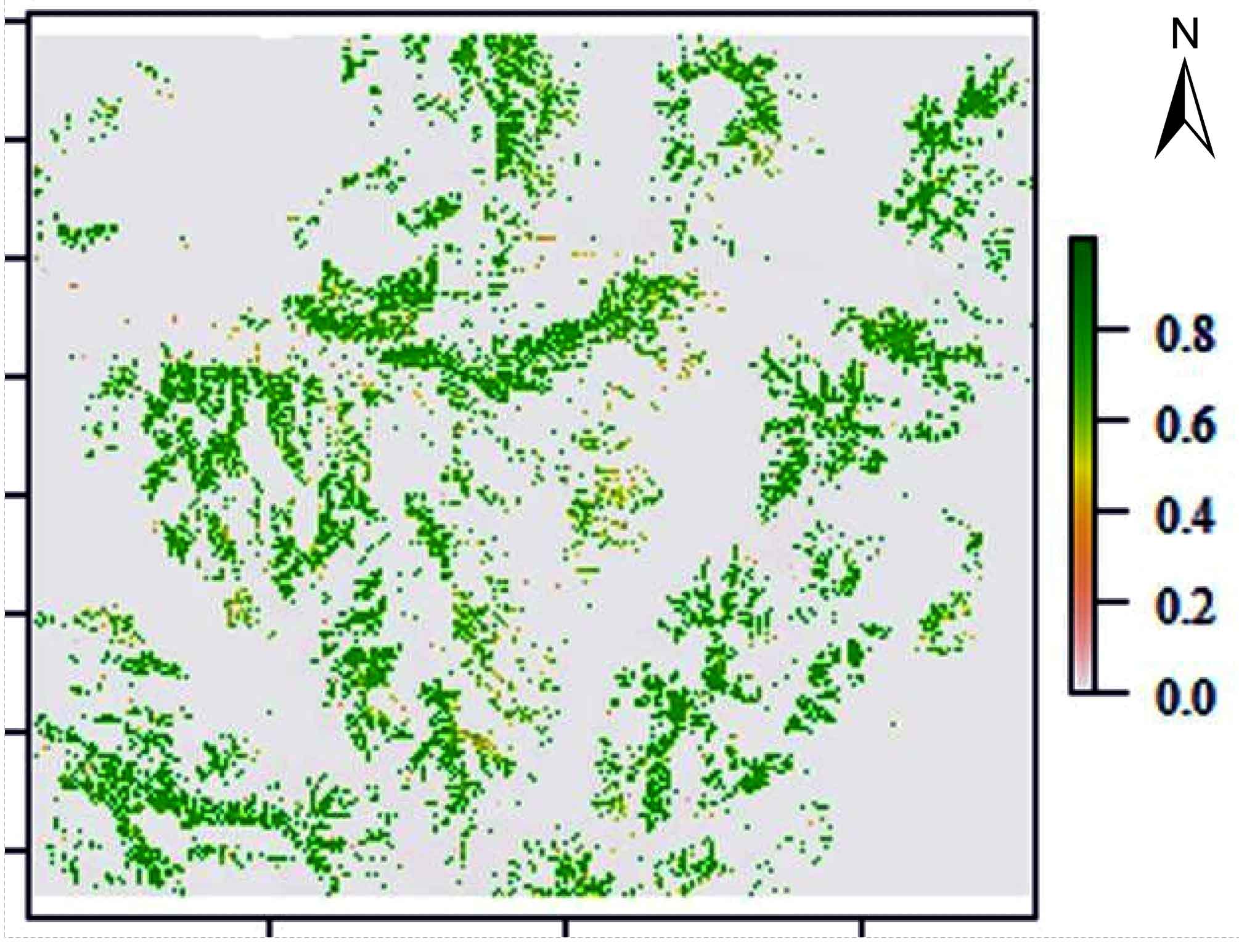
4.5 Landslide Susceptibility Map Along the Road Corridors

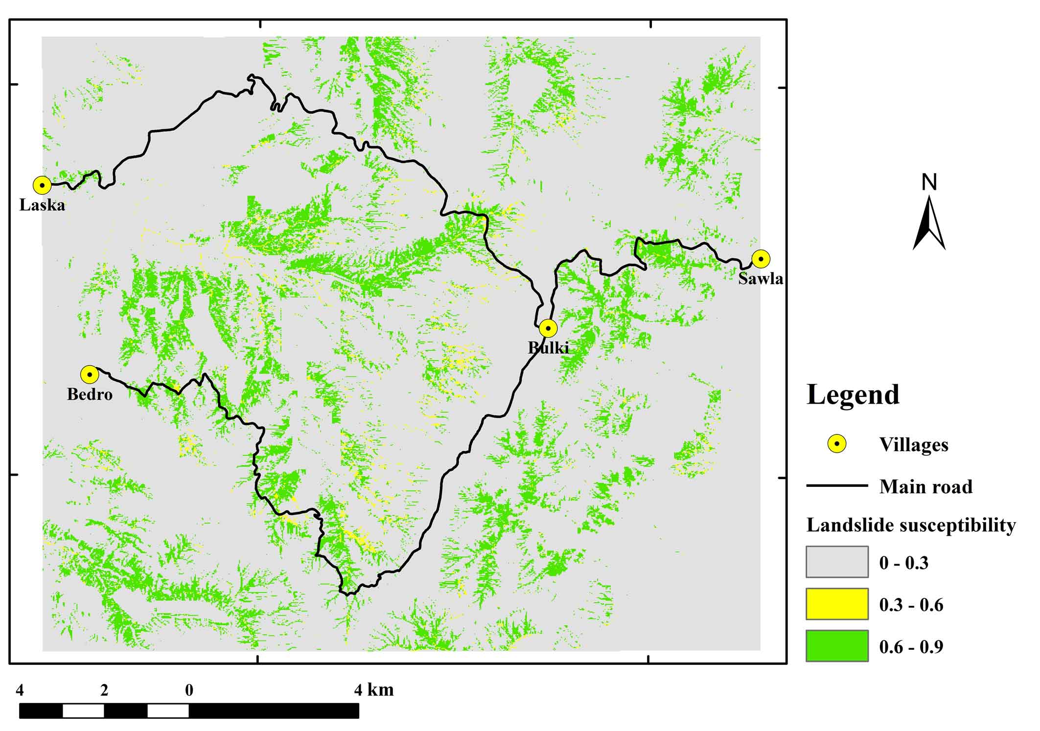
During the model training phase, the model was trained on the current landslide issues. Landslide susceptibility was predicted for the research area based on the attained model performance by merging model learning outcomes with all thematic rater values. In general, the results of the landslide susceptibility map shown in (Figure 15), which depicts future landslides that are likely to occur. Since the model was trained using a scaled dataset between 0 and 1, landslide susceptibility results ranged from 0 to 1.  The likelihood of a landslide occurring is great when the number is one or close to 1, and it lowers as the value approaches 0. Each landslide susceptible model was assigned to one of three susceptibility classes: low, medium, and high susceptible zones. Figure 16 shows the reclassification of the map into three categories: low (0-0.30), medium (0.30-0.60), and high (0.60-0.99) based on the relative percentages area of these classes for each model. Table 5 presents the most of the region 183.85 km² or 75% is divided into lowly susceptible zones, followed by moderately susceptible zones 14.55 km² or 6%, and highly susceptible zones 47.6 km² or 19.34%. According to the findings, landslides are likely to occur in the area’s central region and along its road corridor, mainly due to extensive human activity along these areas’ steep terrain corridors and poor land-use planning. Figure 16 shows a map of the entire region’s susceptibility to landslides. Defining the landslide in terms of the crucial components that are at risk is also helpful. As a result, data on landslide susceptibility along the road corridor recovered the area’s most severely impacted feature. Figure 17 depicts the severity of landslides over different stretches of the route. This led to the identification of about seven road segments that passed through the settlements of Sawla-Bulki, Bulki-Satconcamp, Satconcamp-Geltsa1, Geltsa1-Geltsa2, Geltsa2-Laska, Bulki-Anko, and Anko-Bedro. The road segments between Sawla and Bulki, Bulki and Satconcamp, Geltsa and Laska, and Anko and Bedro were all very prone to slope instability, as shown in (Figure 17). These parts are primarily unstable due to lousy road cuttings, inadequate drainage systems, weak soil conditions, and human activities like farming along the road corridors.

Figure 15. Landslide susceptibility map of ANN model

Figure 16. Landslide susceptibility map

Figure 17. Landslide susceptiblity intensity along the road corridors

5 . DISCUSSION

Various variables and methods can be used to pinpoint areas prone to landslides (Chimidi et al., 2017; Mengistu et al., 2019; Mersha and Meten, 2020). The occurrence, role of determining factors, and model performance of landslides, well-known natural hazards with a complex and nonlinear character, differ from location to location. A few studies on landslide susceptibility have utilized artificial neural networks (ANN) due to their modeling and comprehension capabilities (Won, 2003; Neaupane and Achet, 2004; Ermini et al., 2005; Senise et al., 2013). In this study, an ANN model was trained using 80% of the training datasets. Weight values were calculated by calculating the error between the responses obtained by propagation and the real value of the output, which was previously known. The first through fourth learning stages achieved a minimum RMS error of 22.356866e + 02, 1.169658e + 02, 2.770010e + 01, and 5.677242 e + 02, respectively. Four training phases were accomplished. In order to model landslide susceptibility, the ANN structure’s fourth learning phase, which produced the lowest learning error, was used. This demonstrates that the network learning capability was improved by utilizing two strategies: raising the hidden numbers and lowering input factors thought to lower learning capacity (Lee et al., 2004). According to Senise et al. (2013), expanding the hidden layer can result in a system that is too complicated, which reduces the processing machine’s capabilities. Landslides occur more frequently in sloping, agricultural, and arid areas in the current research area than elsewhere. These were also discovered by the GW and PW analyses, with the slope emerging as the most important contributing component, with a significant rank of 0.75 on its own. Similar results showed a substantial correlation between the prevalence of landslides and agriculture, bare ground, and nearby variables (road, drainage, and lineament). These results are from regional geology, poor soil qualities due to heavy rainfall episodes, human activities along the hilly slope, and poor land use planning along the road corridor (Mengistu et al., 2019; Shano et al., 2021).

According to several authors, the following challenges are raised about landslide susceptibility modeling: (1) Chen et al. (2018) assumed that these models (MLR, SVM, and ANN) couldn’t be used and needed to be validated for detailed planning and assessment purposes. As a result, extreme caution should be used when using these models for specific site characterization, and the scale of the analysis should be carefully considered. (2) The landslide susceptibility models depend on the variables used to implement the models.  Zhou et al. (2018) concluded that the machine learning models (SVM and ANN) are excellent in both the landslide and rockfall susceptibility assessment. Their study demonstrates that the machine learning models are also applicative in complex nonlinear problem, where the SVM model has a better performance due to its globally optimal solution. However, landslide susceptibility maps can significantly guide general planning and evaluation (Lee et al., 2017). Additionally, these methods are constructive and practical for landslide management, hazard analysis, and risk assessment (Wu et al., 1996; Huabin et al. 2005). The receiver operating characteristic curve (ROC) and area under the curve (AUC) statistical measurements were used in this work to assess the effectiveness of the model learning and prediction processes. First, 80% of the landslide dataset with extracted landslide grid pixels were used to assess the model’s learning performance. Second, a 20% testing dataset that was not used during the training phase was used to evaluate the model’s prediction performance. In landslide susceptibility investigations, ROC and AUC statistical measures have been widely employed (Chen et al., 2017; Zhu et al., 2018). Furthermore, the results of our study were quite similar to those of (Elkadiri et al., 2014), who employed ANN and logistic regression (LR) modeling to assess Jazan’s sensitivity to debris flows and had an AUC of 94%. According to their findings, both models’ prediction accuracy is 96.1% and 96.3%, respectively. AUC quantitatively reflects the model’s efficacy in predicting landslide susceptibility, while ROC curves look at the likelihood of correctly classifying the landslide and non-landslide cells. The model’s learning success rate and prediction rate, measured in numbers, were 94% and 88%, respectively. The model’s prediction ability is in the very excellent performance area, where in the literature, AUC >64% and AUC >80% signify good and very good, respectively (Yesilnacar and Topal, 2005). This demonstrated the model’s capacity to comprehend current issues and forecast the research area’s landslide susceptibility pattern in the future. The ANN technique provides the best prediction power in this regard.

Landslide susceptibility maps are capable to help produce a crucial guide for general planning and assessment purposes (Chimidi et al., 2017). These techniques are very useful and practical for landslide management, landslide hazard and risk analysis (Mohamed and Reza, 2021; Mekonnen et al., 2022). In a GIS setting, the susceptibility to landslides is modeled in ranges from 0 to 1, which are then subdivided into low, medium, and high susceptibility zones. Low 183.85 (75%), medium 14.55 (6%), and high 47.6 (19.34%) are the susceptibility grades that correspond to the area covered. High altitude, central, and road corridor-following places are where you’ll typically find susceptible regions. Poor land-use planning procedures and uncontrolled hydrology along the steep terrain are to blame. Due to the combined effects of poor soil, poor hydrology, rough topography, and poorly managed construction work, most current road routes could be more stable. Landslide susceptibility is modeled from 0 to 1 susceptibility ranges, which are further reclassified into low, medium, and high susceptibility zones in a GIS environment. Highly susceptible areas are mainly found following road corridors, in places in the central part, and at high altitudes. This is due to poor land use planning practices and uncontrolled hydrology along the steep terrain. Most existing road corridors are unstable due to the integrated effects of poor soil, poor hydrology, rugged topography, and unmanaged construction work. Additionally, since there is less human activity in areas with flat topography, they remain stable, whereas people are moving to hilly and unstable regions for housing and agricultural purposes. Similar conditions were described in studies conducted in the southwest Ethiopian highlands and close to the rift margin (Mengistu et al., 2019; Shano et al., 2021). This study successfully applied a proposed ANN model for landslide prediction. Nevertheless, comparative research combining two or more methodologies is necessary for better decision-making (Chen et al., 2017; Fang et al., 2021; Mohamed and Reza, 2021; Mekonnen et al., 2022).

6 . LIMITATIONS AND RECOMMENDATIONS

The results section shows that there are a limited number of publications, and there are also many limitations in landslide susceptibility mapping research in Ethiopia. The use of machine learning algorithms for landslide susceptibility mapping is limited in Ethiopia. Landslide evaluation and zonation are challenging tasks because landslides are complex processes that occur because of the influence of several causative and triggering factors. The most important aspect of landslide evaluation is the identification and evaluation of possible causative and triggering factors that may be responsible for initiating landslides in an area. A detailed national landslide inventory database is required to contain all types of information on landslides in Ethiopia, produce a national landslide inventory database, and update it regularly. Based on the results of the present study, it is recommended that areas that fall into high-susceptibility grades require attention by local administration. Furthermore, landslide susceptibility maps, generated using ANN can be applied by decision-makers, planners, and engineers to identify landslide-prone areas, prevent and mitigate landslide risk areas, and determine suitable land-use planning areas, which can be applied to other regions prone to landslides to help reduce the risk of such natural disasters.

7 . CONCLUSION

Owing to its unique capacity to assess spatial correlation data without requiring rigorous statistical assumptions, the application of ANNs modelling in landslide susceptibility analyses has emerged as a legitimate substitute for statistical methods. Deep-learning technology has advanced significantly in recent years. Due to its extraordinarily high categorization accuracy, it has been successfully employed in numerous disciplines including human perceptions and environmental simulations. The deep-learning approach is a reliable strategy for studying landslide susceptibility. The findings and field investigations indicate that the primary landslide danger in the study area is caused by poor land-use practices along roads, rivers, and uneven terrain. In recent years, deep learning technology has developed rapidly. Due to its high classification accuracy, it has been successfully applied in many fields such as human perception and environmental simulation. In landslide susceptibility research, the deep learning method has proven to be reliable. The primary landslide-causing factors were determined to be slope, proximity, and land-use factors (agricultural, bare land, and sparse vegetation). Therefore, this map of landslide susceptibility shows the likely distribution of landslides in the study region and can be used as a guide for additional research and planning of future development activities, such as careful land-use planning, engineering projects, and site selection. However, this study also showed that the area is becoming increasingly prone to landslides. Therefore, careful consideration by planners and other stakeholders is required to include this catastrophic information in the decision-making process. Additionally, the current study demonstrated that the model accurately forecasts the entire study area and comprehends the distribution of landslides at the time. As long as we provide machine-learning models with trustworthy datasets, these technologies can solve complicated problems. In contrast, comparative studies are necessary because landslides are complex, nonlinear issues that differ from place to place, and can impact model capabilities. Landslide protection, retention, and anchoring techniques must be implemented to prevent and control landslide disasters at these locations.

Tables

Figures

Conflict of Interest

Acknowledgements

Abbreviations

References