Keywords

Tolerance intervals , Test of hypotheses , BLIE , ME , MLE , Statistical inference

1 . Introduction

In what follows we will assume that the samples of maxima or minima we are dealing with have a Gumbel distribution for maxima \(\mathrm{\Lambda (( x-\lambda )/\delta )}\), sometimes denoted \(\mathrm{\Lambda ( x |\lambda\,,\delta )}\), or for minima \(\mathrm{1-\Lambda \left( - ( x- \lambda ) / \delta \right) .}\)We will deal only with maxima, minima being dealt with, as said by the relation \(\mathrm{min(x_i)= -max(-x_i).}\) Recall that the Gumbel distribution plays a central role in extreme value theory, being sometimes called the extreme value distribution; it is the limit of both Fréchet and Weibull distributions according to  \(\mathrm{\theta \downarrow 0}\) or \(\mathrm{\theta \uparrow 0 }\) in the von Mises-Jenkinson formula and those distributions can be transformed to a Gumbel distribution by simple (but not always convenient) logarithmic transformations.

2 . Characteristics of the Gumbel distribution

As the distribution \(\mathrm{\Lambda (( x-\lambda )/\delta )}\) is not symmetrical, the natural location parameter need not be the mean; also the convenient scale parameter will not be the standard deviation. Define the standardized or reduced random variable as

\(\mathrm{Z= ( X- \lambda ) / \delta ~~or~~X= \lambda + \delta\, Z }\).

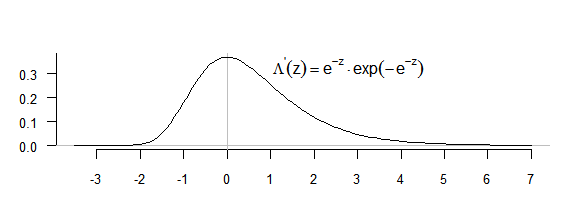
The graph of the probability density  \(\mathrm{\frac{1}{ \delta }e^{- \left( x- \lambda \right) / \delta }exp⁡ ( -e^{ \left( x- \lambda \right) / \delta } ) }\)  for \(\mathrm{\lambda =0~and~ \delta =1}\)  is given in Figure 5.1.

Figure 5.1 Reduced Gumbel density (for maxima)

The moment generating function of \(\mathrm{Z}\) is \(\mathrm{m_{Z} ( \theta ) = \Gamma ( 1- \theta ) }\) \(\mathrm{\left( for~ \theta <1 \right) }\) and that of \(\mathrm{X }\) is \(\mathrm{m_{X} ( \theta) =e^{ \lambda \theta }m_{Z} \left( \delta \theta \right) =e^{ \lambda \theta } \Gamma ( 1- \delta \theta ) \left( \delta \theta <1\right) }\); the corresponding characteristic functions are \(\mathrm{\Phi _{Z} ( t ) = \Gamma ( 1-i~t ) ~and~ \Phi _{X} ( t ) =e^{i \lambda t} \Gamma ( 1-i~ \delta t ) . }\)

All the moments exist as follows from the infinite differentiability of \(\mathrm{\Gamma ( 1-it ) }\). Let us recall that when the mean value \(\mathrm{\mu }\) exists, the central moments (i.e., the moments about \(\mathrm{\mu }\) ) have the expressions, if they exist,

\(\mathrm{ \mu _{i}=M ( \left( X- \mu \right) ^{i} ) }\)

with the variance \(\mathrm{\sigma ^{2}= \mu _{2} }\) and the frequently used linearly invariant measures of skewness and kurtosis,

\(\mathrm{\beta _{1}= \mu _{3}/ \sigma ^{3},~ \beta _{2}= \mu _{4}/ \sigma ^{4}. }\)

In our case we should consider the random variables \(\mathrm{Z}\) and \(\mathrm{X= \lambda + \delta Z }\) with distribution functions \(\mathrm{\Lambda ( z ) ~and~ \Lambda( \left( x- \lambda \right) / \delta ) }\), and the moments and coefficients should be noted \(\mathrm{\mu _{z,i}, }\) and \(\mathrm{\mu _{X,i}, }\) the values of \(\mathrm{\beta_1 }\) and \(\mathrm{\beta_2 }\) being independent of \(\mathrm{ \lambda }\) and \(\mathrm{\delta }\) . We shall, for simplicity, drop the index \(\mathrm{Z }\) always and we have

\(\mathrm{ \mu _{i}= \mu _{Z,i}=M \left( Z- \mu \right) ^{i} }\)

\(\mathrm{ \mu _{X,i}=M \left( Z- \mu _{X} \right) ^{i}= \delta ^{i} \mu _{i}}\)

with \(\mathrm{ \mu _{X}=M ( X ) = \lambda + \delta M ( Z ) = \lambda + \delta _{ \mu }= \lambda + \delta _{ \mu_ Z} }\).

Note also that an analogous relation is valid for quantiles:

if  \(\mathrm{\Lambda ( \chi _{p} ) = \Lambda ( \chi _{Z,p} ) =p }\)  we have \(\mathrm{\chi _{X,p}= \lambda + \delta ~ \chi _{Z,p}= \lambda + \delta~ \chi _{p} }​​\). 

For the mode  \(\mathrm{\mu^{'} }\) , as for the median \(\mathrm{\tilde{\mu} }\) which is the \(\mathrm{.5 }\)-quantile, we have also

\(\mathrm{\mu’_x= \lambda + \delta \mu’_{Z}= \lambda + \delta \mu ’ }\)

and     \(\mathrm{\tilde{\mu}_ x= \lambda + \delta \tilde{\mu} _{Z}= \lambda + \delta \tilde{\mu ~} }\)

We now have the following values for the coefficients associated with \(\mathrm{Z }\), see Gumbel (1958):

\(\mathrm{ \mu _{1}= \gamma =.57722…=Euler’s~constant; }\)  

\(\mathrm{\mu ’=0= \chi _{{1}/{e}};~ }\)

\(\mathrm{\tilde{\mu} =-log\,log\,2=.36651…; }\)

\(\mathrm{\chi _{p}=-log\,log \left( p^{-1} \right) ; }\)  

\(\mathrm{\mu _{2}= \sigma ^{2}={ \pi ^{2}}/{6}=1.64493…; }\)  

\(\mathrm{\sigma =\sqrt[]{ \pi ^{2}/6}=1.28255…; }\)

\(\mathrm{\mu _{3}=2.40411…; }\)

\(\mathrm{\mu _{4}={3 \pi ^{4}}/{20}=14.61136…; }\)

\(\mathrm{\beta _{1}=1.13955; }\)  

\(\mathrm{\beta _{2}=5.40000. }\)   

The return period, for the overpassing the level (or threshold) \({a}\), is, as said before,

\({\mathrm{T}( {a}) = \left( 1- \Lambda \left( ( a- \lambda ) / \delta \right) \right) ^{-1}; }\)

on average \({\mathrm{T}(a) }\) trials will be made until the maximum overpasses \({a}\), after the last overpassing. Note that the probability of overpassing \({a}\) before or at the \(m^{\mathrm{th}}\) trial (year, for instance, if we are thinking of dams) is \(\mathrm{1- \left( 1-p \right) ^{m} }\) where \(\mathrm{p=1- \Lambda \left(( a- \lambda \right) / \delta) }\). Thus is can be written as \({1- ( 1-\frac{1}{\mathrm{T} \left( {a} \right) })^{\mathrm{m}}.}\)

The probability that the overpassing will occur before or at the return period is

\({1- ( 1-\frac{1}{\mathrm{T} \left( a \right) } ) ^{ \left[ \mathrm{T} \left( a \right) \right] }=1-\mathrm{e}^{-1}=.63212 }\) for large \({\mathrm{T}(a) }\) .

The maximum likelihood estimator of \({\mathrm{T}(a) }\) is \({\mathrm{T} ( a ) =\mathrm{N_{k}/k }}\), where \(\mathrm{N_k}\) is the time to the \(\mathrm{k-th}\) occurrence of the overpassing. This is not very convenient and it is better to estimate \({\mathrm{T} ( \left( a- \lambda \right) / \delta ) ~by~\mathrm{T} ( ( a- \hat{\lambda} ) / \hat{\delta} ) , ( \hat{\lambda} , \hat{\delta} ) }\)being the maximum likelihood estimators of \(\mathrm{\left( \lambda , \delta \right) }\) (to be dealt with in the next section), or with other estimators of \(\mathrm{\left( \lambda , \delta \right) }\) .

A simple and useful conservative approximation for \({\mathrm{T}(a) }\), given by Fuller (see Tiago de Oliveira (1972)) is  

\({\mathrm{T} ( a )\mathrm {\approx\tilde{T}}( a ) =\mathrm{exp}\,⁡ \{ \frac{\mathrm{a}- \lambda }{ \delta } \} }\)

with the bounds \({\mathrm{\tilde{T}} ( a ) \leq {\mathrm{T}} ( a ) \leq \mathrm{\tilde{T}} ( a ) ( 1-1/2~\mathrm{\tilde{T}} ( a ) )^{-1}}\).

Usually, when \({\mathrm{T} ( a ) =100 }\),  engineers call \({a}\) “the largest flood in 100 years” or “the 100-years flood”; the expressions in quotes are misnomers because the largest flood in 100 years is a random variable. In a sense, on average, we expect to have to wait 100 years to observe a maximum yearly flood greater than or equal to \({a}\).

From \({\Lambda (( a- \lambda ) / \delta) =1-\frac{1}{\mathrm{T} \left( \left( a- \lambda \right) / \delta \right) } }\)we see that “the 100-year flood” is the \(\mathrm{.99 }\)  quantile.

If a random variable has a Gumbel distribution with parameters \(\mathrm{\lambda , \delta >0 }\) the interval \(\mathrm{\left[ \lambda +b~ \delta , \lambda +a~ \delta \right] }\) has the probability  \(\mathrm{\Lambda \left( a \right) - \left( b \right) }\) and its length is \(\mathrm{ \delta \left( a-b \right) . }\) The shortest interval with a fixed probability \(\mathrm{ \beta }\) is given by the equations (obtained by the Lagrange multipliers method)

\(\mathrm{ \Lambda ( a ) - \Lambda ( b ) = \beta =1- \alpha }\)

\(\mathrm{ \Lambda’ ( a ) -\Lambda’ ( b ) =0 }\)

or    \(\mathrm{ \Lambda( a ) - \Lambda ( b ) = \beta =1- \alpha }\)

\(\mathrm{a+e^{-a}=b+e^{-b}. }\)

A table for some relevant values of is given below.

As could by the expected from the skewness of the distribution the shorted interval is not symmetrical; for instance the shorted intervals containing 90%, 95% and 99% of the population are roughly \(\mathrm{ \left[ \lambda -1.4~ \delta ,~ \lambda +2.5~ \delta \right] , \left[ \lambda -1.6~ \delta , \lambda +3.2~ \delta \right] ~and~ \left[ \lambda -1.9~ \delta ,~ \lambda +4.7~ \delta \right] }\). The interval with\(\mathrm{a=2,~~b=5,~ }\) i.e., \(\mathrm{\left[ \lambda -2~ \delta ,~ \lambda +5~ \delta \right] }\), contains more than 99% of the population.

3 . Point Estimation

The earliest methods of point estimation are the method of moments and the method of maximum likelihood. They were evidently used for Gumbel distribution. Thus these procedures will be given first, followed by some other treatments involving best linear unbiased estimators and best linear invariant estimators.

3.1.Maximum Likelihood Estimators (MLE)

The logarithm of the likelihood of a i.i.d. sample \(\mathrm{\left( x_{1}, x_{2} ,\dots, x_{n} \right) }\)of \(\mathrm{n}\) observations with the distribution function \(\mathrm{\Lambda(( x- \lambda ) / \delta ) }\)is

\(\mathrm{log\,L ( \lambda , \delta \vert x_{i} ) =-n\,log\, \delta - \sum _{1}^{n}e^{- \left( x_{i}- \lambda \right) / \delta }- \sum _{1}^{n} \left( x_{i}- \lambda \right) / \delta . }\)

Setting the partial derivatives of\(\mathrm{​​log \,L}\) with respect to \(\mathrm{​​\lambda}\) and \(\mathrm{\delta}\) equal to zero, we get, with easy algebra, the maximum likelihood equations:

\(\mathrm{\hat{\delta }=\bar{x}- \sum _{1}^{n}x_{i}\,e^{-x_{i}/ \hat{\delta}}/ \sum _{1}^{n}e^{-x_{i}/ \hat{\delta} } }\)

\(\mathrm{\hat{\lambda} =- \hat{\delta} log ( \sum _{1}^{n}e^{-x_{i}/ \hat{\delta} }/n ) . }\)

The second equation is very easy to deal with once the first one is solved. But this one, involving only \(\mathrm{ \hat{\delta} }\), is intractable without computers. One could use an iterative procedure, starting with the moment estimators for \(\mathrm{\lambda }\) and \(\mathrm{{\delta} }\) to follow. However, Kimball developed a simple procedure to get approximate solutions. This is described by him in the sections of Gumbel (1958) which he wrote, summarizing some of his papers. Panchang and Aggarwal (1962) in the “Poona Report” were among the first to use the iterative procedure indicated above, with the use of computers.

Maximum likelihood estimators are asymptotically efficient and unbiased with the variance-covariance matrix given by the inverse of

\(\mathrm{{-n \begin{bmatrix} {M(\frac{\partial^2\,log\,g}{\partial\,\lambda^2})} & \mathrm{M(\frac{\partial^2\,log\,g}{\partial\,\lambda\,\partial\,\delta})} \\[0.3em] \mathrm{M(\frac{\partial^2\,log\,g}{\partial\,\lambda\,\partial\,\delta})} &\mathrm{M}(\frac{\partial^2\,\mathrm{log\,g}}{\partial\,\lambda^2}) \\[0.3em] \end{bmatrix}}}\)

with \(\mathrm{g=g ( x \vert \lambda , \delta ) =\frac{1}{ \delta } \Lambda ’ ( \frac{x- \lambda }{ \delta } ) , }\) the density of Gumbel distribution with parameters \(\mathrm{(\lambda,\delta).}\) It is known that:

The estimators \((\hat{\lambda},\hat{\delta})\) are asymptotically binormal with mean values \((\lambda,\delta),\) the asymptotic variance-covariance matrix is

\(\frac{1}{n}\begin{bmatrix} (1+\frac{6(1-\gamma)^2}{\pi^2})\delta^2 & \frac{6(1-\gamma)}{\pi^2}\delta^2\\[0.3em] \frac{6(1-\gamma)}{\pi^2}\delta^2&\frac{6}{\pi^2}\delta^2 \\[0.3em] \end{bmatrix}\)

and the asymptotic correlation coefficient is

\(\rho (\hat{\lambda},\hat{\delta}) = ( 1+\frac{ \pi ^{2}}{6 \left( 1- \gamma \right) ^{2}} )^ {-{1}/{2}}=.31307. \)

5.3.2.Moments Estimators (ME)

From the relations

\(\mathrm{M ( X ) = \lambda + \delta \gamma }\)

\(\mathrm{ V ( X ) =\frac{ \pi ^{2}}{6}\, \delta ^{2} }\)

we get as estimators by the method of moments

\(\mathrm{\delta ^{*}=\frac{\sqrt[]{6}~~s}{ \pi }=.77970~s }\)

\(\mathrm{\lambda ^{*}=\overline{x}-\frac{\sqrt[]{6}~~\gamma }{ \pi }~s=\overline{x}-.45501~s }\)

where \(\mathrm{\overline{x}}\) and \(\mathrm{s^2}\) are the average \(\mathrm{\left( \sum _{1}^{n}x_{i}/n \right) }\) and the empirical variance \(\mathrm{ ( \sum _{1}^{n}( x_{i}-\overline{x} ) ^{2}/n ). }\)

\(\left( \lambda ^{*}, \delta ^{*} \right)\) is asymptotically binormal but its efficiency is very low (48%); see Tiago de Oliveira (1963). The usefulness of this method, now that computers are used, is to give a simple first estimate as a seed for iteration to solve the maximum likelihood estimator equations.

It should be noted that Gumbel (1958) and Posner (1965) developed methods close to the method of moments (called “simplified” and “modified”), using the plotting positions and a fitted linear regression.

Mann (1968), by simulation and also using Lieblein’s (1954) simulation, has shown that, for estimating quantiles, the Posner (1965) method gives poor estimators for either small or large samples, although the Gumbel (1958) method is relatively good for small samples. The BLUE methods - see below - are preferable.

5.3.3.Best Linear Unbiased Estimators (BLUE)

Lieblein (1954) was the first to recognize that as Gumbel plotting used order statistics, information was wasted if estimators did not use order statistics. He then considered estimating the linear combination

\(\mathrm{\theta = \theta ( a~, b ) =a~ \lambda +b~ \delta ,}\)

with, as special cases, \(\mathrm{ \lambda = \theta \left( 1,0 \right) , \delta = \theta \left( 0,1 \right) }\)and the percentile

\(\mathrm{\theta _{p}= \theta \left( 1, \Lambda ^{-1} \left( p \right) \right) = \lambda + \delta ~ \Lambda ^{-1}( p )}\)

where \(\mathrm{\Lambda ^{-1} \left( p \right) =-log \left( -log~p \right) . }\) He proposed to estimate \(\mathrm{\theta}\) by \(\mathrm{\theta^*}\), a linear combination of order statistics in which the weights are determined to yield minimum variance unbiased estimators. More specifically, \(\mathrm{\theta^*}\)based on double censored data is given by

\(\mathrm{\theta ^{*}= \sum _{i=r+1}^{N-s}w_{i}~x_{i}’ }\)

where, obviously, \(\mathrm{w_i=a\,a_i+b\,b_i.}\) Note that for \(\mathrm{s=r=0}\) we have the complete sample.

The values of \(\mathrm{a_i}\) and \(\mathrm{b_i}\) for which \(\mathrm{M ( \theta ^{*} ) = \theta ~and~V ( \theta ^{*} ) }\) is minimized, are functions of \(\mathrm{n,r,s}\)and may be determined by the generalized least squares procedure of Loyd (1962), based on the generalized Gauss-Markov theorem. As the distribution of order statistics \(\mathrm{Z_i^{'} }\) is parameter-free, the mean values, variances, and covariances depend only on the standardized distribution function and the sample size. For example

\(\mathrm{M\left( Z_{i}^{’~k} \right) =\frac{n~~!}{ \left( i-1 \right) ! \left( n-i \right) !} \int _{- \infty}^{ \infty}z^{k} \Lambda ^{i-1} \left( z \right) \left[ 1- \Lambda \left( z \right) \right] ^{n-1} \Lambda ’ \left( z \right) d~z }\).

Those moments were given numerically by Lieblein (1953).

We start with the fact, observed earlier, because \(\mathrm{X_{i}^{’},= \lambda + \delta ~Z_{i}^{’}~, }\) that

\(\mathrm{M \left( Z_{i}^{’~k} \right) = \lambda + \delta ~ \mu _{i},C ( X_{i}^{’},X_{j}^{’} ) = \delta ^{2} \sigma ’_{ij} }\)

where \(\mathrm{\mu ’_{i}=M \left( Z_{i}^{’} \right) }\) and \(\mathrm{\sigma ’_{ij} }\) is the \(\mathrm{(i,j) }\) the element of the variance-covariance matrix of \(\mathrm{Z= ( Z_{1}^{’},Z_{2}^{’},…,Z_{n}^{’} ) ^{T}.}\) The generalized least squares theorem then states that if \(\mathrm{X}\) is the vector of observations,

\(\mathrm{Z= ( Z_{1}^{’},Z_{2}^{’},…,Z_{n}^{’} ) ^{T}}\)

having \(\mathrm{ M \left( X \right) =A~ \theta }\) with \(\mathrm{ \theta = \left[ \lambda , \delta \right] ^{T}, }\) and \(\mathrm{ C \left( X \right) =C \left( \lambda + \delta ~z \right) = [ \sigma ’_{ij} ] \delta ^{2}=V~ \delta ^{2} }\) where \(\mathrm{A=[\begin{array}{c} \mathrm{1} \\ \mathrm{\mu_1^{'}} \end{array}~\begin{array}{c} \mathrm{1} \\ \mathrm{\mu_2^{'}} \end{array}~...\begin{array}{c} \mathrm{1} \\ \mathrm{\mu_n^{'}} \end{array}~]^T,}\) both \(\mathrm{ A }\) and \(\mathrm{ V }\) being known and \( \mathrm {det \left( V \right) \neq ~0, }\) the least squares estimator of the vector \( \mathrm {\theta = \left[ \lambda , \delta \right] ^{T} }\) is the value that minimizes

\(\mathrm{ \left( X-A~ \theta \right) ^{T}~ V^{-1} \left( X-A~ \theta \right) . }\)

The minimum solution is the one that satisfies the so-called normal equations,

\( \mathrm {~A^{T}~V^{-1}A~ \theta ^{*}=A^{T}~V^{-1}~X }\)            and so

\( \mathrm {\theta ^{*}= \left( A^{T}~V^{-1} A \right) ^{-1} A^{T}~V^{-1}~X }\)

and the variance-covariance matrix of \(\mathrm{\theta^*}\) being

\(\mathrm{C \left( \theta ^{*} \right) = \left( A^{T}~V^{-1} A \right) ^{-1} \delta ^{2} }\)

The estimator \(\mathrm{\theta^*}\) is unbiased and the \(\mathrm{{\theta_i}^*}\) have minimum variance in the class of unbiased linear statistics.

Calculation of the mean values variances and covariances of the order statistics  \(\mathrm{Z_i^{'}}\) and the weights \(a_i,b_i\) are tedious and require computers even for small values of \(n\). They are now tabulated by Mann (1967) (Appendix C) to \(\mathrm{ N=2 \left( 1 \right) 25 , r=0 , s=0 \left( 1 \right) N-2, }\) after some previous work by Lieblein and Zelen (1956)

3.4.Best Linear Invariant Estimators (BLIE)

The unbiased condition of the previous section can be relaxed by defining loss as the mean squared error divided by \(\mathrm{\delta ^{2} }\) and by considering weighted sums of \(\mathrm{Z_{i}^{’}, i=1,2, \dots, r \leq n, }\) as estimators of \(\mathrm{\left( \lambda , \delta \right) }\) and of the quantiles with mean squared error, invariant under translations and multiplications. The estimators among those with smallest mean squared error were called the best linear invariant estimators. The BLUE of Lieblein and Zelen (1956) are also invariant. Mann (1968) has shown that those estimators of \(\mathrm{\left( \lambda , \delta \right) }\) and of the quantiles, are linear functions of the BLUE of \(\mathrm{ \lambda }\) and \(\mathrm{ \delta }\). The mean squared errors of the BLIE are uniformly less than those of the corresponding BLUE, Mann (1968). She says that when \(\mathrm{ r<<n, }\) the ratios of the mean losses of the BLUE relative to those of the corresponding ones of the BLIE are large; for \(\mathrm{ r=2, n=2 \left( 1 \right) 25}\) the mean losses of the BLUE of \(\mathrm{ \lambda }\) and \(\mathrm{ \delta }\) increase with \(\mathrm{n }\) from \(\mathrm{ .659~to~8.24~and~.712~to~.980, }\) respectively. The corresponding ranges of losses when the BLIE are used are \(\mathrm{.657~to~4.49~and~.416~to~.495. }\)

Furthermore, for \(\mathrm{m=2,}\) the losses of the BLIE of the quantiles and \(\mathrm{ \delta }\) are evidently less than or equal to those of the corresponding MLE, which are also invariant. Tables of weights for obtaining the BLIE and the losses of the estimators are available in Mann (1967), (Appendix C).

Asymptotically efficient linear estimators of location and dispersion parameters were obtained and shown to be asymptotically normal by Chernoff et al. (1967). They are invariant and quite efficient with respect to the BLUE, even for fairly small \(\mathrm{n }\), Mann (1968). Johns and Lieberman (1966) used this procedure to determine the weights in the asymptotically efficient linear estimators of \(\mathrm{ \lambda }\) and \(\mathrm{ \delta }\), but there exist (or existed) computer difficulties in comparing the losses of those methods as moment calculations (mean values, variances and covariances) of order statistics involve large rounding errors, requiring multiple-precision computing techniques. Some comparison, based on limited computation, appears in Mann (1968).

3.5.Further methods of linear point estimation

Other approximating methods exist to generate the weights for linear estimators of \(\mathrm{\left( \lambda , \delta \right) }\).

We will enumerate some of them, giving sufficient references; in general they do not need, as does Johns and Lieberman’s (1966) procedure, the tedious and error-prone computation of the first and second moments of order statistics.

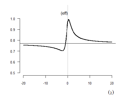
A method of splitting the sample at random in blocks of \(\mathrm{ 4,5~or~6, }\) computing the averages of the blocks, estimating the parameters \(\mathrm{\left( \lambda , \delta \right) }\) from those averages with convenient coefficients, and averaging the estimates, was developed by Lieblein and Zelen (1956) and also studied in Tiago de Oliveira (1972). It was shown there that the asymptotic efficiency for the estimator \(\mathrm{ \chi _{X,p}^{*}= {\lambda} ^{*}+ \chi _{p}\, \delta ^{*} }\) of the quantile \(\mathrm{\chi _{p}}\) has the expression

\(\mathrm{eff( \chi _{X,p}^{*} ) =\frac{1+.60793 \left( .42278+ \chi _{p} \right) ^{2}}{6 \left( .19117+.06274~ \chi _{p}+.13196~~ \chi _{p{2}} \right) } }\)

having as \(\mathrm{\chi _{p} \rightarrow \pm ~ \infty }\) the limit value 0.77, with \(\mathrm{eff ( \chi _{X,1/e}^{*} ) =.97 }\) for the mode and \(\mathrm{eff ( \chi _{X,p}^{*} ) >.77 }\) for \(\mathrm{\chi _{p}>-~.99802 }\) whose probability is \(\mathrm{\Lambda \left( -.98 \right) =.066. }\) See in Figure 5.2 the graph of the efficiency.

Figure 5.2 Asymptotic efficiency of Lieblein - Zelen method

Let us also refer to a method due to Downton (1966), developed for Gumbel minima distribution, now translated to the maxima data.

Denoting by \(\mathrm{\bar{x}= \sum _{1}^{n}x_{i}/n~and~~\bar{w}=\frac{2}{n \left( n-1 \right) } \sum _{1}^{n}i~x_{i}^{’}, }\) where \(\mathrm{x_i' }\) are the usual order statistics, we know that and \(\mathrm{\bar{x} }\) and \(\mathrm{\bar{w} }\) have mean values \(\mathrm{\lambda + \gamma ~ \delta }\) and \(\mathrm{\lambda + ( \gamma +\frac{ n-1}{n+1} log~2 ) ~ \delta . }\) The unbiased estimators

\(\mathrm{\lambda ^{*}=x- \gamma ~ \delta ^{*} }\)

\(\mathrm{\delta ^{*}=\frac{n+1}{ \left( n-1 \right) ~log~{2}} \left( \bar{w}-x \right) }\)

(note that \(\mathrm{\bar{w} ​​>\bar{x}}\)) have the asymptotic efficiency for the estimation of the p-quantile

\(\mathrm{eff \left( \chi _{X,p} \right) =\frac{1+.60793 \left( .42278+ \chi _{p} \right) ^{2}}{1.112825+.459414~ \chi _{p}^{2}+.804621~ \chi _{p}^{2}} }\)

with a graph analogous to the previous one.

See also Tiago de Oliveira (1972) for details. In this paper it was also searched the asymptotically best sample quantiles \(\mathrm{\pi}\) and \(\mathrm{\pi ’ \left( 0< \pi < \pi ’<1 \right) }\) such that the variance of the estimators \(\mathrm{\lambda ^{*}=a~x_{ \pi }^{’}+ \left( 1- a \right) x_{ \pi ’}^{’}, \delta ^{*}=b \left( x_{ \pi ’}^{’}-x_{ \pi }^{’} \right) , }\) was minimum. The correct results (the ones in the paper had a computation error) are \(\mathrm{ \pi =.07, \pi ’=.76, a=-~.43065, b=.44032~ }\) and the asymptotic efficiency is \(\mathrm{eff \left( \lambda ^{*}, \delta ^{*} \right) =40.8 \%}\). For more details see in the Chapter 9 the section “Estimation using two or three quantiles”.

Blom (1958) and in Saharan and Greenberg (1962) developed the nearly best unbiased linear estimators (NBULE) making use of the quantiles \(\mathrm{\Lambda ^{-1} \left( i/ \left( n+1 \right) \right) }\) with relation to the order statistics \(\mathrm{X_i^{'}}\), which Hassanein (1964) applied to the Gumbel distribution. The method can be extended to any distribution having only location and dispersion parameters, directly or by transformation.

Lieblein (1954) proposed a technique using a finite number (in general 3) of empirical quantiles. Hassanein (1964) increased the number of quantiles to be used for the estimation of \(\mathrm{ \lambda }\) and \(\mathrm{ \delta }\). With the sub-sample \(\mathrm{( x_{a_1}^{’} , x_{a_2}^{’}, \dots,x_{a_k}^{’} )~where~1 \leq a_{1}<a_{2}<\dots<a_{k} \leq n, }\) for \(\mathrm{k=2 \left( 1 \right) 10 }\), and with the results of Ogawa (1951), he determined the quantiles to be used which maximize the joint efficiency of the estimators.

Recently Kubat and Epstein (1980) sought the sets of 2 (or 3) order statistics \(\mathrm{x_{r}^{’} }\) and \(\mathrm{x_{r'}^{’} }\) with \(\mathrm{\left( 1 \leq r= \left[ n \pi \right] <r’= \left[ n\pi’ \right] \leq n \right) }\) and coefficients \(\mathrm{ a }\) and \(\mathrm{ b }\), such that \(\mathrm{ \left( \lambda ^{*}, \delta ^{*} \right) }\) with \(\mathrm{ \lambda ^{*}=a~x_{r}^{’}+ \left( 1-a \right) x_{r’}^{’}, \delta ^{*}=b \left( x_{r’}^{’}-x_{r}^{’} \right) }\)were asymptotically unbiased, asymptotically binormal, and with the best efficiency that could be attained to estimate a quantile \(\mathrm{\chi _{p} }\) with  \(\mathrm{\pi <p< \pi ’. }\)

Let us refer in greater detail to the method of block partitioning, which seems simple to execute and does not depend on knowledge of the coefficients of linear combination of the observations, although it needs, once and for all, the computation of efficiency and the best choice of splitting points; see Kubat (1982) for other modifications. The method can be extended to Fréchet and Weibull distributions, as will be seen later.

Take \(\mathrm{r<s }\) such that \(\mathrm{1<r<s <n.}\) The averages are

\(\mathrm{\bar{x}_{1}=\frac{1}{r} \sum _{1}^{r}x_{i}^{’}<\bar{x}_{2}=\frac{1}{s-r} \sum _{r+1}^{s}x_{i}^{’}<\bar{x}_{3}=\frac{1}{n-s} \sum _{s+1}^{n}x_{i}^{’} , }\) with probability \(\mathrm{1.}\)

It can be shown that \(\mathrm{ \left( \bar{x}_{1},\bar{x}_{2},\bar{x}_{3} \right) }\) is asymptotically trinormal and we can seek coefficients \(\mathrm{ a_j }\) and \(\mathrm{ b_j(j=1,2,3) }\) such that the random pair

\(\mathrm{ \lambda ^{*}= \lambda ^{*} \left( x_{i} \right) = \sum _{1}^{3}a_{i}~\bar{x}_{i} }\)

\(\mathrm{ \delta ^{*}= \delta ^{*} \left( x_{i} \right) = \sum _{1}^{3}b_{i}~\bar{x}_{i} }\)

which is always asymptotically binormal has minimum variance; the condition of invariance (i.e., such that \(\mathrm{ \lambda ^{*} \left( \alpha + \beta ~x_{i} \right) = \alpha + \beta ~ \lambda ^{*} \left( x_{i} \right) , \delta ^{*} \left( \alpha + \beta ~x_{i} \right) = \beta ~ \delta ^{*} \left( x_{i} \right) , \left( \beta > 0 \right) }\)implies\(\mathrm{ \sum _{1}^{3}a_{i}=1 }\)) \(\mathrm{ \,and\,\sum _{1}^{3}b_{i}=0. }\) Then we can seek the best \(\mathrm{ r }\) and \(\mathrm{ s }\) in terms of efficiency and thus compute the \(\mathrm{a_i}\) and \(\mathrm{b_i}\).

4 . Further comments

As is well known, the method of maximum likelihood is asymptotically the best and its use is to be recommended.

The other methods (from the moments and the various linear estimators) are not asymptotically efficient and can be considered either as quick methods, if we use only a calculator (and tables if needed), or as a seed for the iterative solution of the \(\mathrm{ \hat{\delta} }\)  equation. If we do not use tables of coefficients, the most practical methods are those of moments — as said with efficiency 48% -or the linear methods with 2 quantiles of Tiago de Oliveira (1972) and of Kubat and Epstein (1980) or of Downton (1966).

5 . Confidence interval estimation

In principle we should always use the maximum likelihood estimator, either for the p-quantile also with a confidence interval, or for the parameter point.

The maximum likelihood estimator \(\mathrm{ \hat{\lambda} + \chi _{p}~ \hat{\delta} }\) is asymptotically normal with mean value \(\mathrm{ \lambda + \chi _{p}~ \delta }\) and variance \(\mathrm{ ( 1+\frac{6}{ \pi ^{2}} \left( 1- \gamma + \chi _{p} \right) ^{2} ) ^{{1}/{2}} \frac{ \delta ^{2}}{n}. }\)

As 

\(\mathrm{ \sqrt[]{n}\frac{( \hat{\lambda} + \chi _{p}~ \hat{\delta}) - ( \lambda + \chi _{p}~ \delta ) }{ ( 1+\frac{6}{ \pi ^{2}} \left( 1- \gamma + \chi _{p} \right) ^{2} ) ^{{1}/{2}} ~\delta } }\)

is asymptotically standard normal and, as \(\mathrm{{\hat{\delta}}\stackrel{\mathrm{P}}{\rightarrow}\delta }\), by the \(\mathrm{\delta }\)-method we know that:

\(\mathrm{\sqrt[]{n} \frac{ ( \hat{\lambda} + \chi _{p}~ \hat{\delta} ) -( \lambda + \chi _{p}~ \delta ) }{ ( 1+\frac{6}{ \pi ^{2}} ( 1- \gamma + \chi _{p} ) ^{2} ) ^{{1}/{2}}~ \hat{\delta} }}\) is asymptotically standard normal, which gives a simple confidence interval for \(\lambda + \chi _{p}~ \delta\) independent of the parameter \(\mathrm{\delta }\) as did not happen with the first asymptotic relation.

We could also compute the bias of estimator of the p-quantile \(\mathrm{M ( \hat{\lambda} - \lambda ) +M ( \hat{\delta} - \delta ) \chi _{p} }\) as well as its variance \(\mathrm{V ( \hat{\lambda} + \chi _{p}~ \hat{\delta} ) =V ( \hat{\lambda } ) +2~C ( \hat{\lambda} , \hat{\delta} ) \chi _{p}+V ( \hat{\delta} ) \chi _{p}^{2} }\). It seems that the bias converges to zero as \(\mathrm{O(n^{-1}) }\)  when the variance converges to zero as \(\mathrm{O(n^{-1}) .}\)

As a result of the asymptotic binormality of \(\mathrm{ ( \hat{ \lambda} , \hat{\delta } ) }\),  the asymptotic confidence interval with significance level \(\mathrm{\alpha }\) for \(\mathrm{\left( \lambda , \delta \right) }\) is given by the curve in the \(\mathrm{\left( \lambda , \delta \right) }\) plane

\(\mathrm{( \hat{\lambda} - \lambda ) ^{2}-2( 1- \gamma ) ( \hat{\lambda} - \lambda ) ( \hat{\delta} - \delta ) + [ \frac{ \pi ^{2}}{6}+ ( 1- \gamma ) ^{2} ] ( \hat{\delta} - \delta ) ^{2} \leq -\frac{2}{n} ~log ~\alpha\cdot \delta ^{2} }\),

that is,

\(\mathrm{ ( \hat{\lambda} - \lambda ) ^{2}-0.84556 ( \hat{\lambda} - \lambda ) ( \hat{\delta }- \delta ) +1.82367 ( \hat{\delta} - \delta ) ^{2} \leq -\frac{2}{n}~log~ \alpha \cdot\delta ^{2}; }\)

recall that the quadratic form of a binormal distribution has the exponential distribution; see Cramér (1946).

Also from \(\mathrm{{\hat{\delta}}\stackrel{\mathrm{P}}{\rightarrow}\delta }\) and by the \(\mathrm{\delta}\)-method we can have asymptotically a part of the ellipsis \(\mathrm{\left( as~ \delta >0 \right)}\)

\(\mathrm{( \hat{\lambda} - \lambda ) ^{2}-2( 1- \gamma ) ( \hat{\lambda} - \lambda ) ( \hat{\delta} - \delta ) + [ \frac{ \pi ^{2}}{6}+ ( 1- \gamma ) ^{2} ] ( \hat{\delta} - \delta ) ^{2} \leq -\frac{2}{n} ~log ~\alpha\cdot \hat{\delta} ^{2} }\).

The other estimators given in “Point Estimation” can be used to obtain an interval estimation or to test hypotheses about the parameters. Most of them are asymptotically normal with known asymptotic variances and covariances, so that one can compute asymptotic confidence intervals; in some cases we may resort to Monte Carlo simulation. For more details see Johns and Lieberman (1966) and Herbach (1970). The reliability function \(\mathrm{R \left( x \right) =exp⁡ \{ -exp⁡ \{ -v/ \delta \} \} ,}\) where \(\mathrm{v= \lambda -x,~ }\)  is an increasing function of \(\mathrm{v/ \delta }\) and a lower confidence limit on \(\mathrm{v/ \delta }\) can be used to determine a lower confidence limit on \(\mathrm{R(x), }\) as \(\mathrm{Prob \{ L<v/ \delta \} =Prob \{ exp⁡ \{ -exp \left( -L \right) \} <exp⁡ \{ -exp \left( -v/ \delta \right) \} =R \left( x \right) = \beta . }\) They proposed to use their asymptotically efficient linear estimators of \(\mathrm{v~and~ \delta }\) based on the first \(\mathrm{r }\) order statistics in a sample of \(\mathrm{n }\). Let  \(\mathrm{Y_{i}^{’}=X_{i}^{’}/a }\). Then for estimates of \(\mathrm{v, \delta }\) we use

\(\mathrm{Y_{a}= \sum _{i=1}^{r}a_{i} Y_{i}^{’} , Y_{b}= \sum _{i=1}^{r}b_{i} Y_{i}^{’} . }\)

Let \(\mathrm{V_{a}= \left( Y_{a}-v \right) / \delta , V_{b} = Y_{a}/ \delta }\). The joint distribution of \(\mathrm{ \left( V_{a}, V_{b} \right) }\) is parameter-free. Next define a function \(\mathrm{L(t) }\) with the property that for fixed \(\mathrm{\beta ~,~0< \beta <1, }\) assuming that \(\mathrm{Prob \{ V_{b}>0 \} =1, }\) we have

\(\mathrm{Prob \left( L \left( t \right) <t~V_{b}-V_{a} \right) = \beta }\)        for all  \(\mathrm{t }\).

Then

\(\mathrm{ Prob \{ L \left( Y_{a} / Y_{b} \right) <v/ \delta \} =Prob \{ \left( Y_{a}/Y_{b} \right) <{L}^{-1} \left( v/ \delta \right) \} = }\)

\(\mathrm{=Prob \{ [ \frac{v}{ \delta }<{L}^{-1} ( \frac{v}{ \delta } ) V_{b}-V_{a} ] \} =Prob \{ L [ {L}^{-1} ( \frac{v}{ \delta } ) ] <{L}^{-1} ( \frac{v}{ \delta } ) V_{b}-V_{a} \} = \beta . }\)

Thus \(\mathrm{L \left( Y_{a} / Y_{b} \right) }\) being a lower confidence limit for \(\mathrm{~v/ \delta }\) with confidence coefficient \(\mathrm{\beta }\), correspondingly \(\mathrm{ exp⁡ \{ -exp \{ -L \left( Y_{a} / Y_{b} \right) \} \}}\) is a lower confidence limit for \(\mathrm{R \left( x \right) , }\) also with confidence coefficient \(\mathrm{\beta }\) .

Finally they show that, asymptotically, \(\mathrm{~L}\) and \(\mathrm{\,exp⁡ \{ -exp\{{ -L} \}\} }\) are efficient bounds for \(\mathrm{~v/ \delta }\)  and \(\mathrm{R \left( x \right) . }\) For \(\mathrm{n=10,~15,~20,~30,~50,~100 }\) and with four values of \(\mathrm{r }\) for each \(\mathrm{n }\), they computed Monte Carlo simulations of the distribution of  \(\mathrm{tV_{b}-V_{a} }\) for fixed values of \(\mathrm{t=Y_{a}/Y_{b} }\). Thus they generated tables from which one can obtain the bounds for \(\mathrm{R \left( x \right) }\) for specific \(\mathrm{x~for~ \beta =.5,~.75,~.90,~.95~and~.99. }\) To get a lower bound on \(\mathrm{R^{-1} \left( w \right) }\) we find in the table a value of  \(\mathrm{ exp⁡ \{ -exp \{ -L \left( Y_{a} / Y_{b} \right) \} \}}\) corresponding to \(\mathrm{w }\) which is \(\mathrm{Y_{a}-t~Y_{b} }\) where \(\mathrm{t }\) is the table value of  \(\mathrm{Y_{a}/Y_{b} }\) associated with \(\mathrm{ exp⁡ \{ -exp \{ -L \left( Y_{a} / Y_{b} \right) \} \}}\) for the appropriate confidence level.

6 . Tests of Hypotheses

Hypothesis testing on parameters can be handled, as usual, by relating the acceptance region to the confidence region.

Consequently, the asymptotic test of \(\mathrm{\left( \lambda , \delta \right) = \left( \lambda _{0} , \delta _{0} \right) ~vs.~ \left( \lambda , \delta \right) \neq \left( \lambda _{0} , \delta _{0} \right) }\) with significance level \(\mathrm{\alpha }\), is given by the acceptance region: accept \(\mathrm{ \left( \lambda _{0} , \delta _{0} \right) }\) if this point falls in the interior of the ellipsis given for the confidence region, and reject otherwise.

Concretely, we will use as the acceptance region, for the significance level \(\mathrm{\alpha }\),

 \(\mathrm{ ( \hat{\lambda} - \lambda _{0} ) ^{2}-2 ( 1- \gamma ) ( \hat{\lambda} - \lambda _{0} ) ( \hat{\delta} - \delta _{0} ) + ( \frac{ \pi ^{2}}{6}+ \left( 1- \gamma \right) ^{2} ) ( \hat{ \delta} - \delta _{0} ) ^{2} \leq -\frac{2}{n}~log ~\alpha \cdot \delta _{0}^{2}. }\)  

Here we do not need to substitute \(\mathrm{\delta _{0}^{2}~ }\) by \(\mathrm{\hat{\delta }^{2}~ }\)in the RHS because in the test \(\mathrm{\delta }\) is supposed known.

Evidently we could obtain, by the classical method, the locally most powerful and locally most powerful unbiased tests if one of the parameters, or a relation between them, is fixed; but we would obtain analogous difficulties and, finally, resort to tests based on maximum likelihood estimation with optimal asymptotic behaviour. They can be let as exercises.

Evidently we could also use other estimators such as the ones described previously, but their efficiencies would in general be low.

7 . Point and Interval Prediction

Let us begin by considering the point prediction of the maximum of (the next) \(\mathrm{m }\) observations from a sample of \(\mathrm{n }\). The likelihood of the sample \(\mathrm{ \left( x_{1} , \dots, x_{n} \right) }\) and the (future) maximum \(\mathrm{ W=w }\) is evidently

\(\mathrm{ L \left( \lambda , \delta \vert x_{i},w \right) =\frac{1}{ \delta ^{n}}~e^{-n \left( \bar{x}- \lambda \right) / \delta }exp \left( \sum _{1}^{n}e^{- \left( x_{i}- \lambda \right) / \delta } \right) \cdot \frac{m}{ \delta }~e^{- \left( w- \lambda \right) / \delta }e^{-m \left( w- \lambda \right) / \delta }. }\)

We could seek, following Tiago de Oliveira (1966) and (1968), the quasi-linearly invariant predictor \(\mathrm{ p \left( x_{1} , \dots, x_{n} \right) }\)(e.g., the predictor such that \(\mathrm{ p( \alpha + \beta ~x_{i} ) = \alpha + \beta ~p( x_{i}) , \beta >0 }\)) such that \(\mathrm{M \left( w-p \left( x_{i} \right) \right) ^{2} }\) is minimum. The result is not manageable, even using computers, as can be seen from the expression

\(\mathrm{p \left( x_{i} \right) =\frac{ \int _{0}^{+ \infty} \xi ^{n-1}\frac{e^{-n~\bar{x}~ \xi }}{ \left( \sum _{1}^{n}e^{- \xi ~x_{i}} \right) ^{n}}( \gamma +log~m-log \sum _{1}^{n}e^{- \xi x_{i}}+\frac{ \Gamma ^{’}( n ) }{ \Gamma ( n ) } ) ~d~ \xi }{ \int _{0}^{+ \infty} \xi ^{n}\frac{e^{-n~\bar{x}~ \xi }}{ \left( \sum _{1}^{n}e^{- \xi~ x_{i}} \right) ^{n}} d ~\xi } }\).

As the \(\mathrm{ M \left( W \right) = \lambda + \left( \gamma +log~m \right) \delta ~and~ ( \hat{\lambda} , \hat{\delta} ) }\)is asymptotically optimal it is then natural to use, as point predictor, the function \(\mathrm{ p \left( x_{i} \right) = \hat{\lambda} +k~ \hat{\delta } }\) which is quasi-linearly invariant because \(\mathrm{ \hat{\lambda} \left( \alpha + \beta ~x_{i} \right) = \alpha + \beta ~\hat{\lambda} \left( x_{i} \right) ~and~~ \hat{\delta } \left( \alpha + \beta ~x_{i} \right) = \beta ~ \delta \left( x_{i} \right) . }\)  

Using the mean-square error as a measure of distance between the prediction and the (to be) observed value of \(\mathrm{ W=w, }\) we have

\(\mathrm{ MSE( p ) =M( W-( \hat{\lambda} +k~ \hat{\delta} ) ^{2}) =M ( W-M( W) ) ^{2}+M ( \hat{\lambda} +k~ \hat{\delta} -M( W) ) ^{2}=}\)\(\mathrm{ =\frac{ \pi ^{2}}{6} \delta ^{2}+M( \hat{ \lambda} +k~ \hat{\delta } ) - ( \lambda + ( \gamma +log~m ) \delta ) ^{2}. }\)

The mean-square error of the point predictor \(~p \left( x_{i} \right) = \hat{\lambda }+k~ \hat{\delta } \) is asymptotically a minimum for \(k= \gamma +log~m \) and its variance is that of the quantile \(\chi= \gamma +log~m \)  i.e., asymptotically.

\(\mathrm{\frac{ \pi ^{2}}{6} \delta ^{2}+ [ 1+\frac{6}{ \pi ^{2}} \left( \gamma +log\,m \right) ^{2} ] \frac{ \delta ^{2}}{n}.}\)

The determination of prediction regions, also dealt with in the same papers, leads to the same difficulties in computing integrals. Thus we will once more use the maximum likelihood estimators.

Let us now seek, then, one-sided and two-sided prediction intervals based on \(\mathrm{ ( \hat{ \lambda} , \hat{\delta } ) }\), for a prediction level \(\mathrm{\omega }\), in general close to \(\mathrm{1}\).

The most important one-sided prediction interval for the prediction level \(\mathrm{\omega }\), for \(\mathrm{W }\) is \(\mathrm{ W \leq \hat{\lambda} +c~ \hat{\delta} }\)with \(\mathrm{ c }\) such that

\(\mathrm{Prob \{ W \leq \hat{\lambda} +c~ \hat{\delta} \} = \omega }\)

which as

\(\mathrm{ Prob\{ W \leq y\} =\Lambda ^{m}{ (( y- \lambda ) }/{ \delta ) }= \Lambda ( ( {y- \lambda ) }/{ \delta } ) -log~m }\)

is reduced to

\(\mathrm{ M ( \Lambda ( \frac{ \hat{\lambda} +c~ \hat{\delta} - \lambda }{ \delta }-log~m ) ) = \omega . }\)

Evidently the first approximation to \(\mathrm{c}\) is from the relation \(\mathrm{\Lambda \left( c - log~m \right) = \omega ~or~c = \chi _{ \omega }+log\,m. }\) Consider now the approximation \(\mathrm{ c= \chi _{ \omega }+log~m+\frac{ \varphi}{\sqrt[]{n}} +O ( n^{-1/2}) . }\) Let us put\(\mathrm{ \sqrt[]{n} \frac{ \hat{\lambda}- \lambda }{ \delta }=A_{n},\sqrt[]{n}~ ( \frac{ \hat{\delta }}{ \delta }-1 ) =B_{n}. }\) Then we get

\(\mathrm{ M ( \Lambda ( \frac{ \hat{\lambda} +c~ \hat{\delta }- \lambda }{ \delta }-log~m )) =M ( \Lambda ( c-log~m+\frac{A_{n}+c~B_{n}}{\sqrt[]{n}} )) = \omega . }\)

Developing \(\mathrm{c}\)  through \(\mathrm{ \chi _{ \omega }+log~m+\frac{ \varphi }{\sqrt[]{n}} +O ( n^{-1/2} ) }\) we get the equation, by easy algebra,

\(\mathrm{\varphi +M \left( A_{n} \right) + \left( \chi _{ \omega }+log \,\omega \right) M \left( B_{n} \right) +O \left( n^{- {1}/{2}} \right) =0, }\)

and as \(\mathrm{ M \left( A_{n} \right) \rightarrow 0~and~M \left( B_{n} \right) \rightarrow 0 }\) we get \(\mathrm{ \varphi =0. }\) Thus \(\mathrm{ c= \chi _{ \omega }+log~m+O \left( n^{-1/2} \right) , }\) or \(\mathrm{ c= \chi _{ \omega }+log~m }\) with a linear error of the order of \(\mathrm{ O \left( n^{-1/2} \right) }\). The prediction level differs from \(\mathrm{ \omega }\) in terms of \(\mathrm{ ( O( n^{-1/2} ) ) ^{2}=O \left( n^{-1} \right) }\) which shows that \(\mathrm{ c= \chi _{ \omega }+log~m }\) gives a good approximation to the quantile with an error in the prediction level of the order \(\mathrm{ O( n^{-1} ) . }\) Consequently:

The one-sided prediction interval with prediction level \( \omega \), to the order of \( O \left( n^{-1/2} \right) \) is, \(\hat{\lambda} + \left( \chi _{ \omega }+log~m \right) ~ \hat{\delta} ~with~ \Lambda \left( \chi _{ \omega } \right) = \omega . \)

 A subsequent summand \(\mathrm{\Psi /n }\) of order \(\mathrm{n^{-1} }\) could be obtained in the same way supposing now that \(\mathrm{\sqrt[]{n}~M \left( A_{n} \right) \rightarrow 0 }\) and \(\mathrm{\sqrt[]{n}~M \left( B_{n} \right) \rightarrow 0; }\) we have then \(\mathrm{\Psi =\frac{1+log\, \omega }{2}( 1+\frac{6}{ \pi ^{2}} \left( 1- \gamma + \chi _{ \omega } + log~m \right) ^{2} ) }\) and so the second order approximation to  \(\mathrm{c}\), with a linear error of the order of  \(\mathrm{ O( n^{-1} ) }\), is

\(\mathrm{ c= \chi _{ \omega }+log\,m+\frac{1+log\,\omega }{2n} ( 1+\frac{6}{ \pi ^{2}} \left( 1- \lambda + \chi _{ \omega }+log\,m \right) ^{2} ) }\)

and the prediction level differs from \(\mathrm{ \omega }\) by a quantity of \(\mathrm{ O \left( n^{-3/2} \right) }\).

The other one-sided interval can be dealt with in the same way.

Let us sketch two-sided prediction intervals with prediction level \(\mathrm{ \omega }\) and asymptotically shortest average length. If \(\mathrm{ a’ \leq b’ }\) are quantities such that

\(\mathrm{ Prob ( \hat{\lambda} +a’~ \hat{\delta} \leq X \leq \hat{\lambda} +b’~ \hat{\delta} ) =w }\)

and \(\mathrm{ b’-a’ }\)  is minimum, they are given by the equations

\(\mathrm{ a’+e^{-a’}=b’+e^{-b’}. }\)

It is then easy to show that if \(\mathrm{ a \leq b~ }\)and are such that

\(\mathrm{ Prob ( \hat{\lambda} +a~ \hat{\delta} \leq W \leq \hat{\lambda} +b~ \hat{\delta} ) =\omega }\)

we shall have \(\mathrm{ ​​​​​​​​​​​a=a’+log~m, b=b’+log~m, }\)apart from terms of order \(\mathrm{n^{-1}}\) with the length \(\mathrm{\left( b-a \right) \delta = \left( b’- a’ \right) \delta}\) which is asymptotically shortest on average.

Other estimators of \(\mathrm{(\lambda,\delta)}\) can be considered as well to form predictors.

8 . Miscellaneous Results

8.1.Discrimination

Consider that we have two populations whose distribution functions are \(\mathrm{\Lambda \left( \left( x- \lambda \right) / \delta \right) }\) and \(\mathrm{\Lambda \left( \left( x’- \lambda ’ \right) / \delta \right) ,}\) where the scale parameter is the same.

Consider that we want to decide if some observation \(\mathrm{y }\) belongs to the first or the second population (i.e., has the location parameter \(\mathrm{\lambda ~or~ \lambda ’ }\)). Supposing \(\mathrm{\lambda ~,~ \lambda ’ }\) and \(\mathrm{\delta }\) to be known, we are in a situation analogous to usual Neyman-Pearson theory for testing hypothesis. Denoting by \(\mathrm{A~and~A’=~A^{c} }\) the acceptance regions for \(\mathrm{\lambda ~and~ \lambda ’ }\), the misclassification errors of the test are

\(\mathrm{Prob{ \{A \vert \lambda ’ \}} = \int _{A} d~ \Lambda ( \frac{y- \lambda ’}{ \delta }) }\)

and     \(\mathrm{Prob{ \{A’ \vert \lambda \}} = \int _{A’} d~ \Lambda ( \frac{y- \lambda }{ \delta } ) =1- \int _{A}d~ \Lambda ( \frac{y- \lambda }{ \delta } ) . }\)

To be fair we stipulate these misclassification errors to be equal, i.e.,

\(\mathrm{\int _{A} [ d~ \Lambda ( \frac{y- \lambda }{ \delta } ) +d~ \Lambda ( \frac{y- \lambda ’}{ \delta } ) ] =1 }\)

and minimize the (equal) misclassification errors \(\mathrm{\int _{A} d~ \Lambda ( \frac{y- \lambda ’}{ \delta } ) . }\)

This test, by the Neyman-Pearson theorem, has the acceptance region for \(\mathrm{ \lambda }\),

\(\mathrm{ \frac{\frac{1}{ \delta }~ \Lambda ’ ( \frac{y- \lambda ’}{ \delta } ) }{\frac{1}{ \delta }~ \Lambda ’ ( \frac{y- \lambda }{ \delta } ) +\frac{1}{ \delta }~ \Lambda ’ ( \frac{y- \lambda ’}{ \delta } ) } \leq k }\)

or                                            

\(\mathrm{ e^{-y/ \delta } ( e^{ \lambda / \delta }-e^{ \lambda ’/ \delta } ) \leq c \left( \lambda , \lambda ’, \delta \right) . }\)

Suppose that \(\mathrm{ \lambda > \lambda ’. }\) Then the acceptance region \(\mathrm{A}\) is given by \(\mathrm{y>c \left( \lambda , \lambda ’, \delta \right) , }\) where \(\mathrm{c}\) is defined by

\(\mathrm{\Lambda ( \frac{c- \lambda }{ \delta } ) + \Lambda ( \frac{c- \lambda ’}{ \delta } ) =1 }\)

and the misclassification error is given by

\(\mathrm{\int _{A} d~ \Lambda ( \frac{y- \lambda ’}{ \delta } ) =1- \Lambda ( \frac{c- \lambda ’}{ \delta } ) ;}\)

if \(\mathrm{ \lambda > \lambda ’ }\) the changes are obvious.

As \(\mathrm{\lambda ~,~ \lambda ’ }\) and \(\mathrm{\delta }\) are not known it is natural to estimate them and substitute in the previous relations.

For a sample of \(\mathrm{ \left( x_{1}, \dots, x_{n} \right) }\) of the first population and of  \(\mathrm{ \left( x_{1}^{’}, \dots, x_{n}^{’} \right) }\) of the second one, the maximum likelihood estimators are

\(\mathrm{ \hat{\hat{\lambda}} =- \hat{\hat{\delta}}~log\frac{ \sum _{1}^{n}e^{-x_{i}/ \hat{\hat{\delta}}}+ \sum _{1}^{n’}e^{{-x’}_{i}/ \hat{\hat{\delta}} }}{n+n’} }\)

and

\(\mathrm{\hat{\delta} =\frac{n}{n+n’} ( \bar{x}- \frac{ \sum _{1}^{n}x_{i} \,e^{-x_{i}/ \delta }}{ \sum _{1}^{n}e^{-x_{i}/ \delta }} ) +\frac{n’}{n+n’} ( \bar{x}’ -\frac{ \sum _{1}^{n’}x’_{i}\,e^{-{x’}_{i} / \hat{\delta} }}{ \sum _{1}^{n’}e^{-{x’}_{i} /\hat{\delta} }} ) . }\)

Thus we substitute \(\mathrm{ \lambda ,~ \lambda ’~and~ \delta }\) by their estimators in the fair test above, taking for \(\mathrm{A}\) the discrimination region corresponding to the largest estimated location parameter.

For more details and the analysis of the asymptotic behaviour (consistency) see Tiago de Oliveira (1973).

8.2.Tolerance intervals

The concept of tolerance intervals was introduced by Wilks (1941) as a procedure for the prediction of the values of a population. In Themido (1985), parameter-free tolerance intervals for the Gumbel distribution are obtained and a comparison, for large samples, is made with the distribution-free tolerance intervals proposed by Wilks, a comparison based on the respective expected lengths.

Let \(\mathrm{ \left( x_{1}, \dots, x_{n} \right) }\) be an i.i.d. sample of one-dimensional continuous random variables, and \(\mathrm{ L_{i}=L_{i} \left( x_{1},\dots , x_{n} \right) , }\)\(\mathrm{ i=1,~2 }\), be statistics such that \(\mathrm{ L_{1} \left( x_{i} \right) <L_{2} \left( x_{i} \right) . }\) The random interval \(\mathrm{\left[ L_{1}, L_{2} \right] }\) is a \(\mathrm{\left( \beta , \omega \right) }\)-tolerance interval if

\(\mathrm{Prob \{{ Prob [ L_{1} \leq X \leq L_{2} ] \geq \beta} \}= \omega , }\)

\(\mathrm{ \omega }\) being the tolerance level of the interval; if, instead of this relation, we have

\(\mathrm{M ( Prob \left[ L_{1} \leq X \leq L_{2} \right] ) = \alpha }\),

the interval \(\mathrm{\left[ L_{1},L_{2} \right] }\) is an \(\mathrm{\alpha }\)-average tolerance interval.

In the first case for given \(\mathrm{\beta ~and~ \omega \left( 0< \beta , \omega <1 \right) }\), we seek tolerance limits \(\mathrm{ L_{1}\,and\,~L_{2} ,}\) based on the sample, such that \(\mathrm{\left[ L_{1},L_{2} \right] }\) contains, with probability \(\mathrm{ \omega }\) at least \(\mathrm{ 100~ \beta ~ \% ~}\)of the populations or such that we have a confidence of \(\mathrm{ 100~ \beta ~ \% ~}\) that the probability that a future observation will lie between \(\mathrm{ L_{1}\,and\,~L_{2} }\) is at least \(\mathrm{ ~ \beta ~}\) ; for the second case we must find \(\mathrm{ L_{1}\,and\,~L_{2} }\) such that the average of mean coverage of the interval is \(\mathrm{\alpha \left( 0< \alpha <1 \right) . }\)

If we have \(\mathrm{L_{1}=- \infty~or~L_{2}=+ \infty }\) we obtain one-sided tolerance intervals.

Regarding the distribution function of the \(\mathrm{X_i}\) we should consider two situations:

• the non-parametric case where the functional form of the distribution of the \(\mathrm{X_i}\) is unknown, apart from the fact that it is (absolutely) continuous; 
• the parametric case where the functional form of the distribution of the \(\mathrm{X_i}\) is known and only the values of a finite number of parameters of the distribution are unknown.

For the determination of tolerance intervals for one-dimensional distributions in the non-parametric case, an exact solution, using order statistics, was given by Wilks (1941).

In the parametric case it is natural to expect that tolerance limits better than those of Wilks can be obtained.

For the Gumbel distribution \(\mathrm{\Lambda ( x \vert \lambda , \delta ) = \Lambda ( \left( x- \lambda \right) / \delta ) ,- \infty< \lambda <+ \infty,0< \delta <+ \infty, }\)let us use as tolerance limits the maximum likelihood estimators of the quantiles of probabilities \(\mathrm{P_{i}= \Lambda ( k_{i} ) ,i=1,2,L_{i}=L_{i} ( x_{1},\dots,x_{n} ) =\hat{ \lambda} +k_{i\,} \hat{\delta} ,with\,k_{1}and\,k_{2} ( k_{1}<k_{2} ) }\)real coefficients independent of \(\mathrm{ n }\), a choice made because \(\mathrm{\hat{ \lambda} ( x_{i} )\, and\, \hat{\delta } ( x_{i} ) }\) are optimum estimators of \(\mathrm{ \lambda }\) and \(\mathrm{\delta }\) in terms of asymptotic efficiency. Recall that \(\mathrm{ \hat{\lambda} +k\, \hat{\delta } }\)are the unique quasi-linearly invariant functions of \(\mathrm{ \hat{\lambda} ~and~ \hat{\delta } }\) .

The (random) proportion of the Gumbel distribution covered by the tolerance interval \(\mathrm{\left[ L_{1},L_{2} \right] }\)  is

  \(\mathrm{ P_{1,2}= \Lambda ( \frac{ \hat{\lambda} \left( x_{i} \right) }{ \delta }+k_{2}\frac{ \hat{\delta} \left( x_{i} \right) }{ \delta } ) - \Lambda ( \frac{ \hat{\lambda} \left( x_{i} \right) }{ \delta }+k_{1}\frac{\hat{\delta} \left( x_{i} \right) }{ \delta } ) = }\)

\(\mathrm{ = \Lambda ( \hat{\lambda } \left( Z_{i} \right) +k_{2}\, \hat{\delta} ( Z_{i} ) ) - \Lambda ( \hat{ \lambda } \left( Z_{i} \right) +k_{1} \hat{\delta} ( Z_{i} ) ) , }\)

where \(\mathrm{ ( z_{1},\dots,z_{n} ) }\)is the corresponding random sample from the reduced Gumbel distribution. This follows from the invariance of maximum likelihood estimators and from the form of the quasi-linearly invariant tolerance limits considered. Thus, the probability \(\mathrm{\hat{P}_{1,2}~of~ \left[ L_{1},L_{2} \right] ~ }\)is parameter-free and the \(\mathrm{\left( \beta , \omega \right) }\)-tolerance interval can be written as \(\mathrm{Prob~ \{ \hat{P}_{1,2} \geq \beta \} = \omega . }\) Using the \(\mathrm{\delta }\)-method Tiago de Oliveira (1982) we can show that the asymptotic distribution of \(\mathrm{\hat{P}_{1,2}}\) is normal, as usual, with mean value \(\mathrm{\Lambda ( k_{2} ) - \Lambda ( k_{1} )}\) and variance \(\mathrm{O ( n^{-1} ) . }\) Even if we take \(\mathrm{k_{1} ( n ) =k_{i}+a_{i}\sqrt[]{n}+O ( n^{-1/2} ) }\), the \(a_\mathrm{i}\) can be computed to give a better approximation; details of an analogous approach can be found in Chapter 8.

For each pair \(\mathrm{ \left( \beta , \omega \right) ,0< \beta , \omega <1, }\)there is an infinity of pairs \(\mathrm{(k_1,k_2) }\) such that the tolerance limits \(\mathrm{L_1}\) and \(\mathrm{L_2}\) define \(\mathrm{a( \beta , \omega ) }\)-tolerance interval for the Gumbel distribution. We can determine the minimum length parameter-free \(\mathrm{\left( \beta , \omega \right) }\)-tolerance interval.

Also, in terms of the \(\mathrm{\alpha}\)-average tolerance interval, \(\mathrm{0<\alpha<1,}\) we can seek the one with minimum length.

The parameter-free \(\mathrm{\left( \beta , \omega \right) }\)-tolerance limits and the parameter-free \(\mathrm{\alpha}\)-average tolerance limits, being estimators of quantiles for the Gumbel distribution converge in probability, as \(\mathrm{n \rightarrow + \infty, }\) to the quantiles which are the end-points of the shortest quantile intervals with probability \(\mathrm{\beta ~and~ \alpha}\) respectively. Tolerance intervals thus correspond to the intervals above but with random end-points.

We can also deal with one-sided parameter-free \(\mathrm{\left( \beta , \omega \right) }\)-tolerance interval; in this case we have only one coefficient, \(\mathrm{k_1\,or\,k_2 }\) for lower or upper intervals respectively.

In the comparison for large samples, between distribution-free and parameter-free two-sided tolerance interval for the Gumbel distribution, with respect to the mean length criterion, the parameter-free tolerance interval using the information about the distribution are, as expected, better than distribution-free tolerance interval.

For the proofs, a tabulation of \(\mathrm{(k_1,k_2), }\) and other details, see Themido (1985).

8.3.Multisample analysis

Consider two samples \(\mathrm{\left( x_{1},\dots,x_{n} \right) and ( x_{1}^{’},\dots,x_{n}^{’} ) , }\)for which we assume that they have a Gumbel distribution with parameters \(\mathrm{\lambda ~and~ \lambda ’ }\) and the same parameter \(\mathrm{\delta }\) .We want to test if \(\mathrm{\lambda = \lambda ’ }\) . This is the first step of Multisample Analysis for Extremes, analogous to Analysis of Variance, but practically unsolved for extremes, and the only case that will be dealt with here.

Analogously to what happened to discrimination we have

\(\mathrm{ \hat{\lambda} =- \hat{\delta}\, log\frac{ \sum _{1}^{n}e^{-x_{i}/ \hat{\delta} }}{n}, \lambda ’=- \,\hat{\delta} \, log\frac{ \sum _{1}^{n’}e^{-{x’}_{i} / \hat{\delta} }}{n’} }\)

and

\(\mathrm{\hat{\delta} =\frac{n}{n+n’} ( \bar{x}- \frac{ \sum _{1}^{n}x_{i} \,e^{-x_{i}/ \hat\delta }}{ \sum _{1}^{n}e^{-x_{i}/ \hat\delta }} ) +\frac{n’}{n+n’} ( \bar{x}’ -\frac{ \sum _{1}^{n’}{x’}_{i}\,e^{-{x’}_{i} / \hat{\delta} }}{ \sum _{1}^{n’}e^{-{x’}_{i} /\hat{\delta} }} ) . }\)

if \(\mathrm{\lambda}\) is supposed different from \(\mathrm{\lambda^{'}}\) and

\(\mathrm{ \hat{\hat{\lambda}} =- \hat{\hat{\delta}}~log\frac{ \sum _{1}^{n}e^{-x_{i}/ \hat{\hat{\delta}}}+ \sum _{1}^{n’}e^{-{x’}_{i}/ \hat{\hat{\delta}} }}{n+n’} }\)

\(\mathrm{\hat{\hat{\delta}} =\frac{n~\bar{x}+n’~\bar{x}’}{n+n’}-\frac{ \sum _{1}^{n}x_{i}~e^{-x_{i}/ \hat{\hat{\delta}} }+ \sum _{1}^{n}x’_{i}~e^{-{x’}_{i}/ \hat{\hat{\delta}} }}{ \sum _{1}^{n}e^{-x_{i}/ \hat{\hat{\delta}} }+ \sum _{1}^{n’}e^{-{x’}_{i}/ \hat{\hat{\delta}} }}}\)

if we suppose \(\mathrm{~ \lambda ’=\lambda .}\)

The likelihood ratio criterion leads to the test statistic

\(\mathrm{-2\,log\frac{\begin{array}{c} \\\mathrm{max} \\ \mathrm{\lambda,\delta} \end{array} \left[ L_{n} \left( x \vert \lambda , \delta \right) L_{n’}~ \left( x’ \vert \lambda , \delta \right) \right] }{\begin{array}{c} \\\mathrm{max} \\ \mathrm{\lambda,\lambda^{'},\delta} \end{array} \left[ L_{n} \left( x \vert \lambda , \delta \right) L_{n’}~ \left( x’ \vert ~ \lambda , \delta \right) \right] }= }\)

\(\mathrm{ =2 \{ ( n+n’ t) log\frac{ \hat{\hat{\delta}} }{ \hat{\delta} }+\frac{n ( \bar{x}- \hat{\hat{\lambda}} ) +n’ ( \bar{x}’- \hat{\hat{\lambda}} ) }{ \hat{\hat{\delta}} }-\frac{n ( \bar{x}- \hat{\lambda} ) +n’ ( \bar{x}’-\hat{ \lambda} ’ ) }{ \hat{\delta} } \} }\)

which is asymptotically \(\mathrm{ a~~ \chi ^{2} }\) with one degree of freedom in the hypothesis tested.

8.4.Overpassing probability of a level

Let \(a\) be a level and suppose that \(\mathrm{X}\) has a Gumbel distribution \(\mathrm{ \Lambda ( ( x- \lambda ) / \delta ) }\). Then \( {\mathrm{P} ( a ) =\mathrm{P} ( a \vert \lambda , \delta ) =\mathrm{Prob} \{\mathrm{ X}>a \} =1- \Lambda ( ( a- \lambda ) / \delta ) }\). We will take as estimator of \({\mathrm{P} ( a \vert \lambda , \delta ) , }\) using the estimators \(\mathrm{ (\hat{\lambda} , \hat{\delta} )​​of​​(\lambda,\delta),}\)

\({\mathrm{\hat{P}}( a ) =\mathrm{P}( a|\hat{\lambda} , \hat{\delta}) }\)

and by the use \(\mathrm{\delta }\)-method we have that \({\mathrm{\sqrt[]{n} ( \hat{P}}(a) -{\mathrm{P}} ( a \vert \lambda , \delta ) ) }\) has the asymptotically normal distribution of the linearized expression.

\({\mathrm{\sqrt[]{n}} [ \left( \lambda - \lambda \right) \frac{ {\mathrm{\partial P}} \left( a \right) }{ \partial \lambda }+ ( \hat{\delta} - \delta ) \frac{\mathrm{ \partial P} \left( a \right) }{ \partial \delta } ] = }\)

\({\mathrm{ =\sqrt[]{n}( 1-P}( a) ) \mathrm{( -\,log} \left( 1-\mathrm{P} \left( a \right) \right) [ \frac{ \hat{\lambda} - \lambda }{ \delta }+\frac{a- \lambda }{ \delta }\frac{ \hat{\delta} - \delta }{ \delta } ] . }\)

Its asymptotic mean value is zero and the variance is

\({\mathrm{ V} ( a \vert \lambda , \delta ) = \left( 1-\mathrm{P} \left( a \right) \right) ^{2} \left( \mathrm{log⁡} \left( 1-\mathrm{P} \left( a \right) \right) \right) ^{2} \{ 1+\frac{6}{ \pi ^{2}} ( 1- \gamma +\frac{a- \lambda }{ \delta } ) ^{2} \} . }\)

Also \({\mathrm{\sqrt[]{n}}\frac{\mathrm{\hat{P}} ( a ) -\mathrm{P} ( a ) }{\sqrt[]{\mathrm{V} ( a \vert \lambda , \delta ) }} }\) is asymptotically standard normal even with \({\mathrm{V} ( a \vert \lambda , \delta ) }\) substituted by \({\mathrm{\hat{V}} ( a ) ={\mathrm{V}} ( a|\hat{\lambda} , \hat{\delta}) . }\)

Then, \(\mathrm{\lambda _{ \alpha } }\) denoting as usual the solution of \(\mathrm{N ( x ) =1- \alpha }\), we have

\({\mathrm{Prob \{ \sqrt[]{n}}\frac{\mathrm{\hat{P}} \left( a \right) -\mathrm{P} \left( a \right) }{\sqrt[]{\mathrm{\hat{V}} \left( a \right) }} \geq - \lambda _{ \alpha } \} \rightarrow 1- \alpha ~as~\mathrm{n }\rightarrow \infty }\)                       and thus:

The one-sided asymptotic confidence interval for \(P(a)\) with significance level \(\alpha\)  is

\(0 \leq P( a ) \leq \hat{P} ( a ) +\frac{ \lambda _{ \alpha }}{\sqrt[]{n}}\sqrt[]{\hat{V} ( a ) }. \)

5.8.5.A worked example

Sneyers (1977) gives the following \(\mathrm{ n=35 }\) maximal yearly precipitations from 1938 to 1972 at Uccle, in 1 mm units, for the durations of 24 h, 60 min, 10 min and 1 min.

Experience says Sneyers - and the plotting confirms it - shows that for small durations the maximal precipitation follows a Gumbel distribution but for large durations it follows a Fréchet distribution.

The ML method applied to 1 min duration data gives \(\mathrm{ \hat{\lambda} =1.709286 }\)  and \(\mathrm{ \hat{\delta}=.778273 }\), close to \(\mathrm{ 1.694 }\)  and \(\mathrm{ .7777 }\)  or \(\mathrm{ 1.691 }\)  and \(\mathrm{ .7484 }\) obtained by Sneyers by other methods.

From the values of \(\mathrm{( \hat{ \lambda} , \hat{\delta } ) }\) we can solve other decision problems such as the ones discussed before.

To test the goodness of fit of a known (or fixed) distribution \(\mathrm{F(x)}\) we can use the Kolmogoroff-Smirnov test statistic

\(\mathrm{ KS_{n}=\begin{array}{c} \\\mathrm{sup} \\ \mathrm{x} \end{array}\vert S_{n}( x ) -F ( x ) \vert =\begin{array}{c} \mathrm{n} \\ \mathrm{max} \\ \mathrm{1}\end{array} \{ max( \vert F ( x_{i}^{’})-\frac{i}{n} \vert , \vert F ( x_{i+1}^{’})-\frac{i}{n} \vert) \} , }\)  

where \(\mathrm{S_{n} ( x ) =S_{n} ( x \vert x_{i} )}\) denotes the sample distribution function \(\mathrm{( x_{1}^{’} \leq x_{2}^{’} \leq \dots \leq x_{n}^{’} ) }\) , the order statistics of the i.i.d. sample and is taken \(\mathrm{F ( x_{n+1}^{’} ) =1. }\) We accept \(\mathrm{F(x)}\), at the significance levels \(\mathrm{ .05 }\) and \(\mathrm{ .01 }\), according to \(\mathrm{ \sqrt[]{n}~KS_{n} \leq 1.36~or~\sqrt[]{n}~KS_{n} \leq 1.63 }\), rejecting otherwise. When we assume model  \(\mathrm{ F(x|\theta) }\) , we estimate \(\mathrm{ \theta }\) by \(\mathrm{ \hat{\theta} }\) (say) and instead of the unknown (parameterized) \(\mathrm{ F(x|\theta) }\) we compute \(\mathrm{ \hat{K}S_{n}=\begin{array}{c} \\\mathrm{sup} \\ \mathrm{x} \end{array} \vert S_{n} ( x ) -F ( x \vert \hat{\theta} ) \vert }\)and act in the same way as before. Although the procedure is not completely justified, it can be expected to be sufficiently approximate when \(\mathrm{n }\) is large.

In our case, assuming the Gumbel model, with the values of \(\mathrm{( \hat{ \lambda}, \hat{\delta } ) }\)  above, we have

\(\mathrm{ \hat{K}S_{n}=\begin{array}{c} \\\mathrm{sup} \\ \mathrm{x} \end{array} \vert S_{n} ( x ) - \Lambda (( x- \hat{\lambda} ) / \hat{\delta } ) \vert =.0102432 }\)

and as \(\mathrm{ n=35 }\)  we have \(\mathrm{ \sqrt[]{n}~\hat{K}S_{n}=.06059 }\) , accepting thus the Gumbel model.

Tables

Figures

References