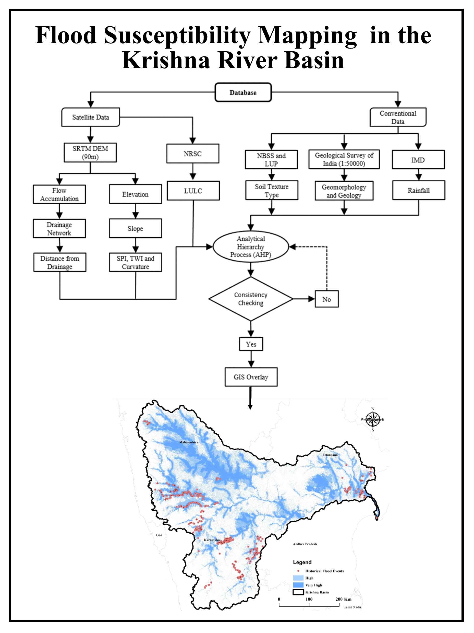
The location map was generated using Shuttle Radar Topography Mission (SRTM) Digital Elevation Model (DEM) data at a 90m resolution, employing the hydrology analysis tools within the ArcMap 10.8 software environment (Figure 1). The freely available SRTM 90m DEM, with a vertical accuracy of ±16 m, has been widely validated and applied in hydrological studies (Farr et al., 2007; Gangani et al., 2023; Bielski et al., 2024). It remains suitable for large-scale basins such as the Krishna, providing adequate accuracy, consistency, and feasibility for regional flood assessment. Key terrain characteristics, containing elevation, slope, curvature, flow accumulation, and drainage networks, were analyzed to construct the drainage density map. River proximity was quantified using spatial buffering techniques in ArcMap. Geospatial data on geology and geomorphology were sourced from the GSI. Rainfall distribution maps were developed utilizing meteorological datasets procured from the Indian Meteorological Department, Pune. Land use and land cover (LULC) mapping was facilitated by Landsat 8-9 Enhanced Thematic Mapper Plus (ETM+) imagery, with a spatial resolution of 30 m. Soil texture information, essential for the soil texture mapping of the Krishna basin, was acquired from the National Bureau of Soil Survey and Land Use Planning (NBSS and LUP), ensuring data precision and integrity. The Topographic Wetness Index (TWI) and Stream Power Index (SPI) were derived directly within the ArcMap framework using the DEM data.
A flood susceptibility assessment has been conducted in the KRB, using a multi-criteria analysis context based on the AHP as proposed by Saaty (1980). The evaluation incorporated a comprehensive set of physiographic criteria, including Elevation, Slope, and Proximity to the river, Geomorphology, Drainage
density, Flow accumulation, Rainfall, LULC, Geology, Soil type, SPI, TWI, and Curvature. This technique offers a rigorous, efficient tactic for detecting flood-prone areas, thereby supporting effective water resource management and mitigation policies within the basin. The analytical procedure comprised six sequential steps: criteria selection, ranking of criteria, pairwise comparison, weight calculation, score assignment, and execution of a weighted overlay analysis. These methodological steps were pivotal in delineating areas susceptible to flooding, thereby enhancing the understanding of flood risk dynamics and informing strategic planning in the KRB.
3.1 Analytical Hierarchy Process (AHP) model
The major factors influencing flood susceptibility include elevation, slope gradient, river proximity, Rainfall, flow accumulation, LULC, geological structure, TWI, and surface curvature. To demarcate the flood prone areas in KRB multiple parameters have been taken into account on the basis of their relative significance in the decision-making method. The structured categorization, optimization of efficiency, and generation of precise outcomes are fundamental attributes of the AHP (Das, 2019; Gaikwad, 2019). The AHP is extensively applied for managing water resources. The analysis rigorously incorporated a comprehensive suite of thirteen physiographic parameters. Each criterion has gave a rank based on its significance, aiding in the organization and prioritization of spatial decisions (Saaty, 1977; Das, 2019; Navale and Bhagat, 2021). The most important criteria were assigned higher weights whereas the least important were given lower weights. The Pairwise Comparison Matrix (PWCM) in AHP assesses factors influencing flood susceptibility using Saaty’s scale (1977), with values ranging from 9 to 1/9 to indicate relative significance. These comparisons help calculate priority weights for decision-making in flood prone mapping. In the present work, criteria were ranked from 1 to 9, with expert input determining the significance of each factor. AHP is an innovative and flexible method in statistics, widely used in research for analyzing multiple factors and predicting outcomes accurately to solve complex problems. The AHP method has been applied to assign weights and ranks to different parameters in the flood prone index model, as shown below:
\(FH = \sum_{i=1}^{n} W_i * R_i\) (1)
Where, FH is the flood hazard index, Wi is the weight of each factor, and Ri is the rank of each factor’s value. The final map in this study is categorized into five classes: very low, low, moderate, high, and very high, using the FH model to assess the probability of flood occurrence (Das, 2018).
AHP calculates parameter weights using the Pairwise Comparison Matrix (PCM) based on the relative importance and influence of each factor on the basis of extensive literature review and the expert opinion. These weights establish the importance of each parameter in a hierarchical structure. After calculating the weights in PCM, the matrix is normalized by dividing respectively judgment value by the total of its column. The quotient values for each row are summed and then divided by the number of parameters in the PCM (Table 1). The resultant value for each parameter represents its weight, extending from 0 to 1, with the sum of all weights constantly equal to 1.
A PCM is established, with diagonal elements set to 1 (Eq. 2). The relative prominence of the criteria has determined based on predefined criteria, assigning ranks as follows: 1 for equally important, 3 for moderately more important, 5 for strongly more important and 7 for very strongly more important. Intermediate values, such as 2, 4, and 6, are used to represent varying degrees of importance (Dejen and Soni 2021). Each row shows how important one parameter is compared to others. For example, the first row compares elevation to eight other parameters. In AHP, parameters deemed more important receive higher numerical weights, while less important ones are assigned reciprocal values. For example, if basin elevation is more significant than slope, it may be assigned 5, with slope receiving 1/5. This reciprocal system ensures consistent and proportional weighting across all parameters for flood-susceptibility analysis (Saaty, 1977; Das, 2018).
The quantitative and qualitative approach is a major strength of AHP (Forman, 1993; Doke et al., 2021).
\(A = (a_{ij})_{n \times n} = \begin{bmatrix} a_{11} & a_{12} & \dots & a_{1n} \\ a_{21} & a_{22} & \dots & a_{2n} \\ a_{n1} & a_{n2} & \dots & a_{nn} \end{bmatrix}, \quad a_{ii} = 1, \quad a_{ij} = \frac{1}{a_{ji}}, \; a_{ij} \ne 0\) (2)
Where,
A: The matrix A represents the collection of all pairwise comparisons between the parameters n × n, indicating a square matrix with n rows and n columns.
\(aij = \) Element at the \(i\) -th row and \(j\) -th column
\(a_{ii}\) =1: Diagonal elements of the matrix are always 1, as each parameter is equally important to itself
\(a_{ij} = \frac{1}{a_{ij}}\) Elements are reciprocals of each other, ensuring consistency in the comparison (if parameter iii is more important than \(j\) , then \(j\) is less important than \(i\) ). \(a_{ij} \neq 0\) : No element in the matrix is zero, as comparisons are always non-zero values.
Afterward, the weighted arithmetic mean methodology is employed to compute the weights in the PCM. In this process, the values in the matrix are standardized to obtain the standardized values in the standard pairwise comparison matrix (Table 2). This normalization step confirms that all values are scaled in a consistent method, facilitating the calculation of relative importance or weights for each parameter. Using Equation (3), the pairwise comparison matrix (Table 1) was normalized by dividing each parameter by its respective column sum, ensuring all column totals equal to 1. The average of each row produced the relative weight of each criterion (Table 2). (Equation 3 and 4).
\(a_{ij} = \frac{a_{ij}}{\sum_{i=1}^{n} a_{ij}}\) (3)
\(w_i = \frac{1}{n} \sum_{j=1}^{n} a'_{ij}\) (4)
\(A_w=λ maxW\) (5)
The equation \(A_w=λ maxW\) is used to find the importance of criteria in decision-making. w is the weight factor and A is a comparison matrix, and. By averaging rows and solving the equation, we determine the relative weights of each criterion (Equation 5).
3.1.1 Consistency ratio (CR)
Consistency in judgments is assessed using the CR calculated as (Biswas et al., 2021),
CR \(=\frac{CI}{RI}\) (6)
Where the Consistency Index,
CI \(=\frac{\lambda_{\text{max}} - n}{n - 1}\) (7)
λ max as the largest eigenvalue and n as the matrix order (Pawluszek and Borkowski, 2017).
Equation (7) was then applied to assess judgment consistency. The maximum eigenvalue ( \(λ_{max}\) =13.78)) was derived from the matrix–weight product, yielding (CI=0.065) and (CR=0.041). As CR < 0.10, the pairwise comparisons are considered consistent and reliable for flood susceptibility analysis in the KRB. Eigenvalues, particularly \(λ_{max}\) , are derived from the sum of total and normalized weights, with Saaty’s RI providing consistency benchmarks, such as 1.56 for 13 criteria. Table 3 represents the AHP method has been applied to a total of 13 parameters and all their subtypes considered for the research, and those parameters have been given a relative ranking according to their importance.
3.2 Preparations of Thematic Layers
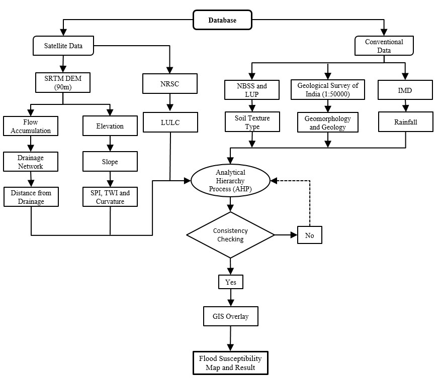
To delineate the flood hazard zones in the KRB, high-resolution satellite imagery and ancillary data were procured from a range of digital repositories and governmental institutions. The detailed methodological framework is illustrated in Figure 2.
3.2.1 Elevation
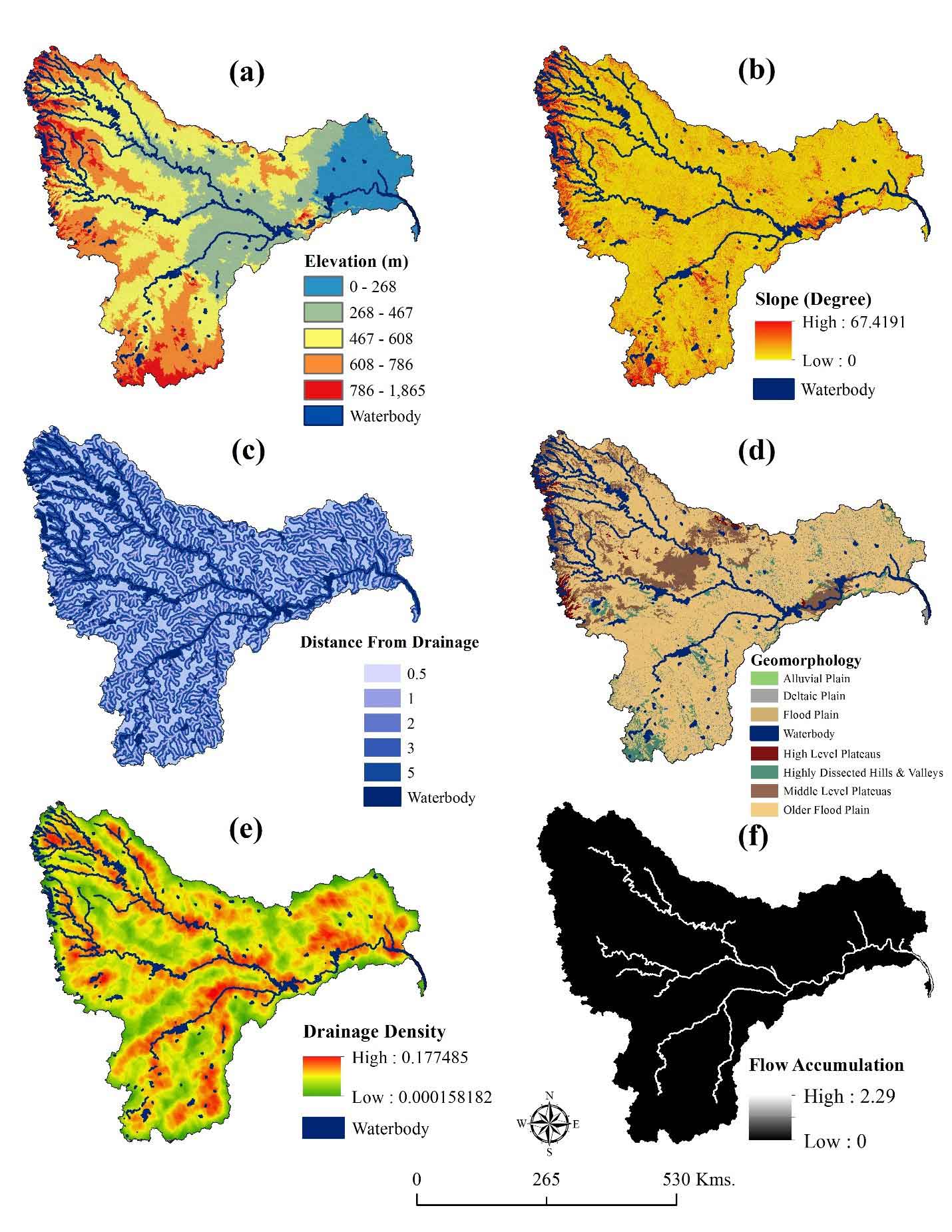
According Botzen et al (2012) elevation is key factor in mapping flood risk vulnerability. High elevated land areas have less risk of flooding, while lowland plains are more vulnerable. The areas at higher elevations exhibits lower flood susceptibility (Tehrany et al., 2013; Das, 2018). The relief in Krishna basin ranges from 0 to 1865m. About 10% of the basin lies around 250m elevation, while nearly 20% of the area falls between 250 and 450m (Figure 3a).
3.2.2 Slope
Mapping flood-susceptible areas, slope is a crucial topographic factor because it controls surface water flow. In the present study area, the slope values range from 0° to 67°. Surface slope acts as an amplifying factor by increasing water-flow velocity and reducing infiltration, which collectively heightens flood risk (Elkhrachy, 2015). As the slope gradient increases, runoff becomes faster and infiltration decreases; however, where the slope suddenly flattens, the reduced flow velocity causes water to accumulate, leading to stagnation and potential flooding (Das, 2019; Doke et al., 2021).
3.2.3 Distance from the river
Proximity to river channels is considered a significant geomorphic factor while preparing accurate scientific maps of flood prone area. The areas closer to the river generally have lower elevation and gentler slopes. Additionally, a river channel represents the lowest topographic point within a given area. Consequently, regions located farther from the river exhibit reduced susceptibility to flooding. In the present study the buffer tool of ArcGIS software is used to calculate the distance from the river (Figure 3c). Multiple buffers were generated at intervals of 0.5km, which were then merged into a single vector layer and subsequently converted into a raster format for further analysis. (Fernandez and Lutz, 2010; Das, 2018). Flooding raises groundwater levels, especially in flat areas, causing prolonged waterlogging and slower drainage. However, the areas near rivers, ponds, and lakes are prone to flooding due to elevation changes, with flash floods also occurring based on meteorological and topographical factors (Pham et al., 2020).
Table 1. Pairwise comparison matrix (PCM)
|
Criteria
|
Elevation
|
Slope
|
Distance from Drainage
|
Geomorphology
|
DD
|
FA
|
RF
|
LULC
|
Geology
|
ST
|
STI
|
TWI
|
Curvature
|
|
Elevation
|
1
|
|
|
|
|
|
|
|
|
|
|
|
|
|
Slope
|
1/2
|
1
|
|
|
|
|
|
|
|
|
|
|
|
|
Distance from Drainage
|
1/3
|
1/2
|
1
|
|
|
|
|
|
|
|
|
|
|
|
Geomorphology
|
1/4
|
1/3
|
1/2
|
1
|
|
|
|
|
|
|
|
|
|
|
DD
|
1/4
|
1/4
|
1/3
|
1/2
|
1
|
|
|
|
|
|
|
|
|
|
FA
|
1/5
|
1/4
|
1/4
|
1/3
|
1/2
|
1
|
|
|
|
|
|
|
|
|
RF
|
1/6
|
1/5
|
1/4
|
1/4
|
1/3
|
1/2
|
1
|
|
|
|
|
|
|
|
LULC
|
1/7
|
1/6
|
1/5
|
1/4
|
1/4
|
1/3
|
1/2
|
1
|
|
|
|
|
|
|
Geology
|
1/8
|
1/7
|
1/6
|
1/5
|
1/4
|
1/4
|
1/3
|
1/2
|
1
|
|
|
|
|
|
ST
|
1/8
|
1/8
|
1/7
|
1/6
|
1/5
|
1/4
|
1/4
|
1/3
|
1/2
|
1
|
|
|
|
|
STI
|
1/9
|
1/8
|
1/8
|
1/7
|
1/6
|
1/5
|
1/4
|
1/4
|
1/3
|
1/2
|
1
|
|
|
|
TWI
|
1/9
|
1/9
|
1/8
|
1/8
|
1/7
|
1/6
|
1/5
|
1/4
|
1/4
|
1/3
|
1/2
|
1
|
|
|
Curvature
|
1/10
|
1/9
|
1/9
|
1/8
|
1/8
|
1/7
|
1/6
|
1/5
|
1/4
|
1/4
|
1/3
|
1/2
|
1
|
Table 2. Standardized pairwise comparison matrix and their weights
|
Criteria
|
Elevation
|
Slope
|
Distance from Drainage
|
Geomorphology
|
DD
|
FA
|
RF
|
LULC
|
Geology
|
ST
|
STI
|
TWI
|
Curvature
|
Weights
|
Weights %
|
|
Elevation
|
0.3096
|
0.3831
|
0.3659
|
0.3309
|
0.2505
|
0.2399
|
0.2247
|
0.2088
|
0.1936
|
0.1630
|
0.1556
|
0.1353
|
0.1316
|
0.2379
|
23.79
|
|
Slope
|
0.1548
|
0.1916
|
0.2439
|
0.2481
|
0.2505
|
0.1919
|
0.1873
|
0.1789
|
0.1694
|
0.1630
|
0.1383
|
0.1353
|
0.1184
|
0.1824
|
18.24
|
|
Distance from Drainage
|
0.1032
|
0.0958
|
0.1220
|
0.1654
|
0.1879
|
0.1919
|
0.1498
|
0.1491
|
0.1452
|
0.1426
|
0.1383
|
0.1203
|
0.1184
|
0.1408
|
14.08
|
|
Geomorphology
|
0.0774
|
0.0639
|
0.0610
|
0.0827
|
0.1252
|
0.1440
|
0.1498
|
0.1193
|
0.1210
|
0.1222
|
0.1210
|
0.1203
|
0.1053
|
0.1087
|
10.87
|
|
DD
|
0.0774
|
0.0479
|
0.0407
|
0.0414
|
0.0626
|
0.0960
|
0.1124
|
0.1193
|
0.0968
|
0.1019
|
0.1038
|
0.1053
|
0.1053
|
0.0854
|
8.54
|
|
FA
|
0.0619
|
0.0479
|
0.0305
|
0.0276
|
0.0313
|
0.0480
|
0.0749
|
0.0895
|
0.0968
|
0.0815
|
0.0865
|
0.0902
|
0.0921
|
0.0660
|
6.60
|
|
RF
|
0.0516
|
0.0383
|
0.0305
|
0.0207
|
0.0209
|
0.0240
|
0.0375
|
0.0596
|
0.0726
|
0.0815
|
0.0692
|
0.0752
|
0.0789
|
0.0508
|
5.08
|
|
LULC
|
0.0442
|
0.0319
|
0.0244
|
0.0207
|
0.0157
|
0.0160
|
0.0187
|
0.0298
|
0.0484
|
0.0611
|
0.0692
|
0.0602
|
0.0658
|
0.0389
|
3.89
|
|
Geology
|
0.0387
|
0.0274
|
0.0203
|
0.0165
|
0.0157
|
0.0120
|
0.0125
|
0.0149
|
0.0242
|
0.0407
|
0.0519
|
0.0602
|
0.0526
|
0.0298
|
2.98
|
|
STI
|
0.0387
|
0.0239
|
0.0174
|
0.0138
|
0.0125
|
0.0120
|
0.0094
|
0.0099
|
0.0121
|
0.0204
|
0.0346
|
0.0451
|
0.0526
|
0.0233
|
2.33
|
|
STI
|
0.0344
|
0.0239
|
0.0152
|
0.0118
|
0.0104
|
0.0096
|
0.0094
|
0.0075
|
0.0081
|
0.0102
|
0.0173
|
0.0301
|
0.0395
|
0.0175
|
1.75
|
|
TWI
|
0.0038
|
0.0213
|
0.0152
|
0.0103
|
0.0089
|
0.0080
|
0.0075
|
0.0075
|
0.0060
|
0.0068
|
0.0086
|
0.0150
|
0.0263
|
0.0112
|
1.12
|
|
Curvature
|
0.0034
|
0.0024
|
0.0136
|
0.0103
|
0.0078
|
0.0069
|
0.0062
|
0.0060
|
0.0060
|
0.0051
|
0.0057
|
0.0075
|
0.0132
|
0.0072
|
0.72
|
Table 3. The pairwise comparison matrix and the weights according to sub-criteria
|
Sr. No
|
Parameter
|
Sub-Class
|
1
|
2
|
3
|
4
|
5
|
6
|
7
|
8
|
9
|
CR
|
Weights
|
Weights (%)
|
|
1
|
Elevation
|
0 – 268
|
1
|
|
|
|
|
|
|
|
|
0.0947
|
0.499
|
50
|
|
|
|
268 – 467
|
1/3
|
1
|
|
|
|
|
|
|
|
|
0.256
|
26
|
|
|
|
467 – 608
|
1/5
|
1/3
|
1
|
|
|
|
|
|
|
|
0.138
|
14
|
|
|
|
608 – 786
|
1/7
|
1/5
|
1/3
|
1
|
|
|
|
|
|
|
0.070
|
7
|
|
|
|
786 – 1865
|
1/8
|
1/6
|
1/5
|
1/3
|
1
|
|
|
|
|
|
0.038
|
4
|
|
2
|
Slope (Degree)
|
0 – 2.1
|
1
|
|
|
|
|
|
|
|
|
0.0788
|
0.393
|
40
|
|
|
|
2.1 – 5.8
|
1/2
|
1
|
|
|
|
|
|
|
|
|
0.296
|
30
|
|
|
|
5.8 – 12.2
|
1/3
|
1/3
|
1
|
|
|
|
|
|
|
|
0.166
|
17
|
|
|
|
12.2 – 21.4
|
1/4
|
1/4
|
1/3
|
1
|
|
|
|
|
|
|
0.093
|
9
|
|
|
|
21.4 – 67.4
|
1/5
|
1/5
|
1/4
|
1/3
|
1
|
|
|
|
|
|
0.051
|
5
|
|
3
|
Distance from Drainage (Km)
|
0 – 0.5
|
1
|
|
|
|
|
|
|
|
|
0.0609
|
0.445
|
45
|
|
|
|
0.5 – 1
|
1/2
|
1
|
|
|
|
|
|
|
|
|
0.297
|
30
|
|
|
|
1 – 2
|
1/4
|
1/3
|
1
|
|
|
|
|
|
|
|
0.147
|
|
|
|
|
2 – 3
|
1/6
|
1/5
|
1/3
|
1
|
|
|
|
|
|
|
0.073
|
7
|
|
|
|
3 – 5
|
1/8
|
1/7
|
1/5
|
1/3
|
1
|
|
|
|
|
|
0.037
|
4
|
|
4
|
Geomorphology
|
Water body
|
1
|
|
|
|
|
|
|
|
|
0.0414
|
0.3070
|
31
|
|
|
|
Flood Plain
|
1/2
|
1
|
|
|
|
|
|
|
|
|
0.2182
|
22
|
|
|
|
Older Flood Plain
|
1/3
|
1/2
|
1
|
|
|
|
|
|
|
|
0.1543
|
15
|
|
|
|
Deltaic Plain
|
1/4
|
1/3
|
1/2
|
1
|
|
|
|
|
|
|
0.1089
|
11
|
|
|
|
Alluvial Plain
|
1/4
|
1/4
|
1/3
|
1/2
|
1
|
|
|
|
|
|
0.0764
|
8
|
|
|
|
Middle Level Plateau
|
1/5
|
1/4
|
1/4
|
1/3
|
1/2
|
1
|
|
|
|
|
0.0533
|
5
|
|
|
|
High Level Plateau
|
1/5
|
1/5
|
1/4
|
1/4
|
1/3
|
1/2
|
1
|
|
|
|
0.0370
|
4
|
|
|
|
Highly Dissected Hills and Valleys
|
1/6
|
1/5
|
1/5
|
1/4
|
1/4
|
1/3
|
1/2
|
1
|
|
|
0.0259
|
3
|
|
5
|
Drainage Density
|
Very High
|
1
|
|
|
|
|
|
|
|
|
0.0341
|
0.464
|
46
|
|
|
|
High
|
1/2
|
1
|
|
|
|
|
|
|
|
|
0.264
|
26
|
|
|
|
Moderate
|
1/4
|
1/2
|
1
|
|
|
|
|
|
|
|
0.149
|
15
|
|
|
|
Low
|
1/6
|
1/4
|
1/2
|
1
|
|
|
|
|
|
|
0.083
|
8
|
|
|
|
Very Low
|
1/8
|
1/6
|
1/5
|
1/2
|
1
|
|
|
|
|
|
0.040
|
4
|
|
6
|
Flow Accumulation
|
77311428 – 228338405
|
1
|
|
|
|
|
|
|
|
|
0.0642
|
0.441
|
4
|
|
|
|
37756744 – 77311428
|
1/2
|
1
|
|
|
|
|
|
|
|
|
0.249
|
25
|
|
|
|
77080431 –37756744
|
1/4
|
1/2
|
1
|
|
|
|
|
|
|
|
0.179
|
18
|
|
|
|
4494850 – 17080431
|
1/5
|
1/3
|
1/3
|
1
|
|
|
|
|
|
|
0.090
|
9
|
|
|
|
0 – 4494850
|
1/6
|
1/5
|
1/5
|
1/3
|
1
|
|
|
|
|
|
0.046
|
4
|
|
|
|
|
|
|
|
|
|
|
|
|
|
|
|
|
|
7
|
Rainfall (mm)
|
< 980
|
1
|
|
|
|
|
|
|
|
|
0.0207
|
0.456
|
46
|
|
|
|
981 - 1315
|
1/2
|
1
|
|
|
|
|
|
|
|
|
0.254
|
25
|
|
|
|
1315 - 1912
|
1/4
|
1/2
|
1
|
|
|
|
|
|
|
|
0.157
|
16
|
|
|
|
1912 - 2773
|
1/5
|
1/3
|
1/2
|
1
|
|
|
|
|
|
|
0.087
|
9
|
|
|
|
>2773
|
1/7
|
1/5
|
1/4
|
1/2
|
1
|
|
|
|
|
|
0.049
|
5
|
|
8
|
LULC
|
Water body
|
1
|
|
|
|
|
|
|
|
|
0.0357
|
0.376
|
38
|
|
|
|
Built-up
|
1/2
|
1
|
|
|
|
|
|
|
|
|
0.246
|
25
|
|
|
|
Westland
|
1/3
|
1/2
|
1
|
|
|
|
|
|
|
|
0.145
|
15
|
|
|
|
Agriculture Land
|
1/4
|
1/3
|
1/2
|
1
|
|
|
|
|
|
|
0.108
|
11
|
|
|
|
Grass Land
|
1/5
|
1/4
|
1/3
|
1/2
|
1
|
|
|
|
|
|
0.064
|
6
|
|
|
|
Forest Land
|
1/6
|
1/5
|
1/5
|
1/4
|
1/2
|
1
|
|
|
|
|
0.043
|
4
|
|
9
|
Geology
|
Deccan Trap
|
1
|
|
|
|
|
|
|
|
|
0.0413
|
0.273
|
27
|
|
|
|
Dharwar
|
1/2
|
1
|
|
|
|
|
|
|
|
|
0.182
|
18
|
|
|
|
Cuddapah
|
1/2
|
1/2
|
1
|
|
|
|
|
|
|
|
0.189
|
19
|
|
|
|
Gondwana
|
1/3
|
1/3
|
1/2
|
1
|
|
|
|
|
|
|
0.123
|
12
|
|
|
|
Granite
|
1/4
|
1/5
|
1/3
|
1/2
|
1
|
|
|
|
|
|
0.085
|
9
|
|
|
|
Kaladgi
|
1/5
|
1/5
|
1/5
|
1/3
|
1/2
|
1
|
|
|
|
|
0.061
|
6
|
|
|
|
Pakhal
|
1/7
|
1/6
|
1/6
|
1/4
|
1/3
|
1/2
|
1
|
|
|
|
0.042
|
4
|
|
|
|
Eastern Ghat
|
1/7
|
1/7
|
1/7
|
1/6
|
1/5
|
1/4
|
1/3
|
1
|
|
|
0.027
|
3
|
|
|
|
Peninsular Gneissic Complex
|
1/8
|
1/7
|
1/7
|
1/7
|
1/6
|
1/6
|
1/4
|
1/3
|
1
|
|
0.018
|
2
|
|
10
|
Soil Texture
|
Clay
|
1
|
|
|
|
|
|
|
|
|
0.0413
|
0.273
|
27
|
|
|
|
Clay Loam
|
1/2
|
1
|
|
|
|
|
|
|
|
|
0.182
|
18
|
|
|
|
Loam
|
1/2
|
1/2
|
1
|
|
|
|
|
|
|
|
0.189
|
19
|
|
|
|
Silty Clay
|
1/3
|
1/3
|
1/2
|
1
|
|
|
|
|
|
|
0.123
|
12
|
|
|
|
Silty Clay Loam
|
1/4
|
1/5
|
1/3
|
1/2
|
1
|
|
|
|
|
|
0.085
|
9
|
|
|
|
Silty Loam
|
1/5
|
1/5
|
1/5
|
1/3
|
1/2
|
1
|
|
|
|
|
0.061
|
6
|
|
|
|
Loamy Sand
|
1/7
|
1/6
|
1/6
|
1/4
|
1/3
|
1/2
|
1
|
|
|
|
0.042
|
4
|
|
|
|
Fine Sand Loamy
|
1/7
|
1/7
|
1/7
|
1/6
|
1/5
|
1/4
|
1/3
|
1
|
|
|
0.027
|
3
|
|
|
|
Sandy Loam
|
1/8
|
1/7
|
1/7
|
1/7
|
1/6
|
1/6
|
1/4
|
1/3
|
1
|
|
0.018
|
2
|
|
11
|
SPI
|
8.9 – 9.5
|
1
|
|
|
|
|
|
|
|
|
0.0947
|
0.499
|
50
|
|
|
|
9.5 – 10.8
|
1/3
|
1
|
|
|
|
|
|
|
|
|
0.256
|
26
|
|
|
|
10.8 – 12.9
|
1/5
|
1/3
|
1
|
|
|
|
|
|
|
|
0.138
|
14
|
|
|
|
12.9 – 16.2
|
1/7
|
1/5
|
1/3
|
1
|
|
|
|
|
|
|
0.070
|
7
|
|
|
|
16.2 – 23.7
|
1/8
|
1/6
|
1/5
|
1/3
|
1
|
|
|
|
|
|
0.038
|
4
|
|
12
|
TWI
|
11.3 – 23.8
|
1
|
|
|
|
|
|
|
|
|
0.0357
|
0.459
|
46
|
|
|
|
8.01 – 11.3
|
1/2
|
1
|
|
|
|
|
|
|
|
|
0.268
|
27
|
|
|
|
5.6 – 8.01
|
1/4
|
1/2
|
1
|
|
|
|
|
|
|
|
0.144
|
14
|
|
|
|
3.7 – 5.6
|
1/6
|
1/4
|
1/2
|
1
|
|
|
|
|
|
|
0.085
|
9
|
|
|
|
-0.7 – 3.7
|
1/7
|
1/6
|
1/4
|
1/3
|
1
|
|
|
|
|
|
0.043
|
4
|
|
13
|
Curvature
|
-3.8 – -2.1
|
1
|
|
|
|
|
|
|
|
|
0.0835
|
0.503
|
50
|
|
|
|
-2.1 – -0.05
|
1/3
|
1
|
|
|
|
|
|
|
|
|
0.260
|
26
|
|
|
|
-0.05 – 0.05
|
1/5
|
1/3
|
1
|
|
|
|
|
|
|
|
0.134
|
13
|
|
|
|
0.05 – 0.25
|
1/7
|
1/5
|
1/3
|
1
|
|
|
|
|
|
|
0.068
|
7
|
|
|
|
0.25 – 3.7
|
1/9
|
1/7
|
1/5
|
1/3
|
1
|
|
|
|
|
|
0.035
|
4
|
3.2.4 Geomorphology
Geomorphology affects both groundwater and flooding by influencing how water moves, collects, and drains in an area. Geomorphology regulates groundwater dynamics by controlling infiltration, storage, and movement, with floodplains enhancing recharge but increasing flood risk, while hilly terrains promote runoff and flash floods (Andualem and Demeke, 2019; Doke et al., 2021). The Figure 3d shows nine geomorphic features of the KRB, including waterbodies, flood plain, older flood plains, deltaic plains, alluvial plains, high-level plateaus, middle-level plateaus, and dissected hills and valleys (Bordoloi et al., 2023). High flood susceptibility in its flood plain, older flood plain, deltaic plain, and alluvial plain due to low elevation, flat topography, and proximity to river systems. The deltaic plain is particularly vulnerable due to tidal influences and sediment deposition. In contrast, high-level plateaus, middle-level plateaus, and dissected hills and valleys facilitate rapid runoff, intensifying downstream flooding.
3.2.5 Drainage density
Drainage density (Dd), defined as the ratio of total drainage network length to total basin area, influences flood risk. Higher drainage density results in faster runoff, lower infiltration and increased flood potential, especial in steep or impermeable areas. Low drainage density allows greater infiltration, reducing flood susceptibility. However, while high Dd increases flood risk, it also aids in rapid water evacuation, with overall impact depending on soil permeability, land use, and rainfall intensity. (Subbarayan and Sivaranjani, 2020; Doke et al., 2021). Hence, higher Dd areas are assigned higher scores due to their greater flood susceptibility, while areas with lower drainage density received lower scores as they have reduced flood risk. The Dd in the study area ranges between 0 to 1.49 km/km². They are divided into five categories to capture finer spatial variations in drainage density and to improve the clarity and accuracy of the flood-susceptibility analysis (Figure 3e).
3.2.6 Flow accumulation
Flow accumulation is defined as concentration of flow within a watershed, representing the sum of upstream area contributing runoff to a specific point. In the downstream region of river, where tributaries converge, the velocity and volume of water increase, which rises the flood potential. Flow accumulation measures drainage areas and increases from high land to river outlets (Schauble et al., 2008). The upstream region of river Krishna the flow accumulation is lesser due to the presence of lower-order streams (Figure 3f). As the river progresses downstream, numerous tributaries merge with the main channel, significantly increasing flow accumulation and flood vulnerability (Krishnan et al., 2025). Therefore, higher flow accumulation in the downstream region increases flood risk (Tehrany et al., 2015; Das, 2018).
3.2.7 Rainfall
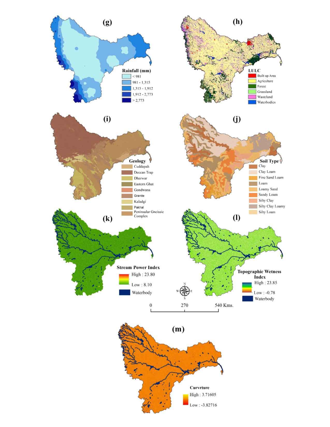
River water level and flow accumulation depends on the intensity, frequency, and amount of rainfall (Dou et al., 2017). Precipitation is the major source of surface water, excluding glacier-fed areas. It plays a crucial role in river flow and flooding, with sudden rainfall, especially in dry regions, potentially triggering flash floods (Das, 2018). However, groundwater is a vibrant natural reserve refilled by precipitation. While intense rainfall enhances surface water penetration, excessive rainwater can decrease the soil’s absorption ability, leading to increased runoff and a greater possibility of flooding (Maity and Mandal, 2019; Doke et al., 2021). The basin receives ~90% of its 859 mm annual rainfall during the southwest monsoon (June–October) (Figure 4g). Orographic lifting of monsoon winds by the Western Ghats (610–2,134 m) causes high rainfall in the western basin, while the eastern regions remain drier (WRIS, 2018). This spatial variability, combined with intense monsoon precipitation, exacerbates flood risks, particularly in downstream areas with inadequate drainage and high sediment loads.
3.2.8 Land use land cover (LULC)
LULC is important for flood risk mapping because it affects surface runoff, infiltration, and the connection between surface water and aquifer (Gigovic et al., 2017; Kazakis et al., 2015). LULC data has been collected from the Bhuvan Portal, a website of the National Remote Sensing Centre ISRO, Hyderabad, India. This dataset is for the period 2019–2020 and has been published under the National Land Use and Land Cover Mapping Project. The maps are based on Level-II classification system and have a scale of 1:50,000. Land utilization patterns in the Krishna Basin are shaped by socio-cultural and economic factors, influencing adaptive land use techniques in response to the natural environment (Das et al., 2017; Kaur et al., 2017). Urban landscape planning plays a vital role in environmental sustainability by supporting better management of land changes over time while mitigating the risks of natural calamities i.e. floods, caused by deforestation and urbanization. (Cetin et al., 2018a; Cetin et al., 2018b; Das et al., 2017). The basin exhibits diverse land use classes, including agriculture (75.86%), natural vegetation (10.04%), wetlands (7.64%), water bodies (4.07%), built-up areas (2.29%), and grasslands (0.11%) (Figure 4h).
3.2.9 Geology
Porosity and permeability, governed by rock lithology, plays a critical role in controlling infiltration, runoff generation, and groundwater flow (Kalita et al., 2025).
Lithology can significantly impact flood behavior particularly in basaltic terrains such as the Deccan Traps where low porosity and limited permeability promote quick surface runoff, reduced infiltration, and unstable channel conditions (Kale and Rajaguru, 1987; Subramanian, 1993; Grover et al., 2024; Terker, 2024). Although precipitation, surface morphology, and land use often exert stronger controls on short-term flood intensity, lithological characteristics still contribute significantly to basin-scale hydrological response. In fact, several recent studies have shown that Deccan basalt formations enhance runoff generation and increase flood susceptibility due to their unique hydraulic properties (Jerin Joe, et al., 2025; Paswan et al., 2025). Geological information for this study was obtained from the GSI, based on digital geological maps at 1:250,000 scale, which provide a reliable overview of lithological variability across the study area. The basin comprises three major geological units the Deccan Trap basalt, Cuddapah sediments, and Dharwad crystalline rocks (Figure 4i). The northwestern Deccan Trap region, dominated by hard basaltic flows, shows low permeability and high runoff, particularly in the upper catchments of the Mula, Mutha, Bhima, Pavana, and Indrayani rivers. In contrast, the Cuddapah region exhibits moderate to high infiltration, supporting groundwater recharge, while the Dharwad crystalline terrain allows deeper percolation due to its fractured bedrock. Additional lithologies such as Gondwana, Granite, Kaladgi, and Pakhal further contribute to the basin’s geological and hydrological diversity.
3.2.10 Soil type
Soil type is a key factor in influencing surface runoff and the infiltration rate of water. Soils with higher clay content than sand, the amount and rate of surface runoff are generally greater (Olii et al., 2021). Soil data has been obtained from the online resource of National Bureau of Soil Survey and Land Use Planning (NBSS and LUP). This dataset is at a scale of 1:250,000 and shows the major soil types and soil properties of the study area. The KRB exhibits various soil classes, such as clay loam, fine sandy loam, loamy sand, loam, and clay, each distributed across different regions of the basin (Figure 4j). Clay loam and clay soils are found in large quantities in the north-western part of the KRB. The presence of the Deccan trap in this region is the rate of erosion intensity and of water velocity is high with water infiltration rate is low (Jain et al., 2007; Patil et al., 2024). Fine sandy loam in the central and eastern parts of the KRB represents mature to old alluvial deposits, where long-term sediment sorting produces smooth, fine-textured soils. These well-developed alluvial surfaces reduce channel roughness and lower river velocity, but their broad, gently sloping floodplains allow the river to carry a higher volume of water (Leopold and Wolman, 1970; Bridge, 2009). The loamy sand soil is situated in the south-western area of the basin, influenced by the Western Ghats, and is shaped by moderate river flow from the tributaries.
3.2.11 Stream power index
The SPI measures the erosive power of water flow (Jebur et al., 2014; Khosravi et al., 2016; Das, 2019; Yilmaz, 2022), assessing the energy available for sediment transport and erosion in rivers. This energy influences channel changes and plays significant role in flood events (Das and Scaringi, 2021). SPI is an important measure of erosion and sediment transport in streams (Fuller, 2008; Barker et al., 2009; Hong et al., 2018). The SPI is calculated using the formula (Moore et al., 1991; Dejen and Soni 2021), as follows:
\(SPI = As\:tanβ \) (7)
Where, As is the specific catchment area, and ???? is the slope gradient.
The SPI of the KRB ranges from 8 to 23.8, indicating variations in flow energy and erosion potential across the watershed (Figure 4k). Higher SPI values suggest areas with intense water flow and increased erosion risk, often corresponding to steep slopes and major drainage channels, while lower values indicate regions with gentle slopes and decreases the flow intensity.
3.2.12 Topographic wetness index
TWI deals with how terrain affects surface water flow accumulation, soil saturation, and soil moisture, with high values in valleys and low values on slopes (Gokceoglu et al., 2005; Yong et al., 2012; Mojaddadi et al., 2017). Flooding is more likely in high TWI areas due to increased soil saturation, rising groundwater, and reduced drainage (Ho-Hagemann et al., 2015). TWI helps identify flood-prone areas by indicating zones with a higher potential for soil saturation, especially where low slopes and large contributing catchments promote water accumulation during heavy rainfall. The TWI is calculated as:
\(TWI=ln(As/tanβ) \) (8)
Where, As = upslope contributing area (m2 m−1), and β = the local slope inclination in degree.
Higher TWI values indicate areas with more water accumulation, which are more prone to flooding and higher soil moisture. Lower TWI indicates drier, well-drained areas with less risk of flooding. TWI values in the KRB range from –0.70 to 23.85. Although TWI is usually positive; negative TWI values represent ridge tops and steep slopes where water quickly runs off and little to no saturation occurs (Figure 4l).
3.2.13 Curvature
Curvature is commonly classified into concave, convex, and flat surfaces (Tehrany et al., 2013). Concave areas facilitate convergent flow, convex areas cause divergent flow, while flat surfaces produce minimal runoff (Costache and Tien, 2019). Curvature therefore helps interpret how terrain shape influences water movement across the landscape (Costache et al., 2020). These characteristics are crucial for hydrological modeling. Curvature also influences flooding: negative values (concave) trap water, positive values (convex) promote drainage, and values near zero indicate flat areas with even water flow (Das, 2018; Cao et al., 2016). In the KRB, the general surface curvature ranges from –3 to 3.7, reflecting variations in overall landform shape that influence water flow, accumulation, and erosion across the basin (Figure 4m). Negative values represent concave areas, which promote water accumulation and increase flood susceptibility, while positive values indicate convex regions, facilitating runoff and reducing flood risk.
All data sets have been unified to a spatial resolution of 90m by transforming them into the same coordinate system, WGS 84 / UTM Zone 43N, thereby maintaining spatial consistency across all datasets.
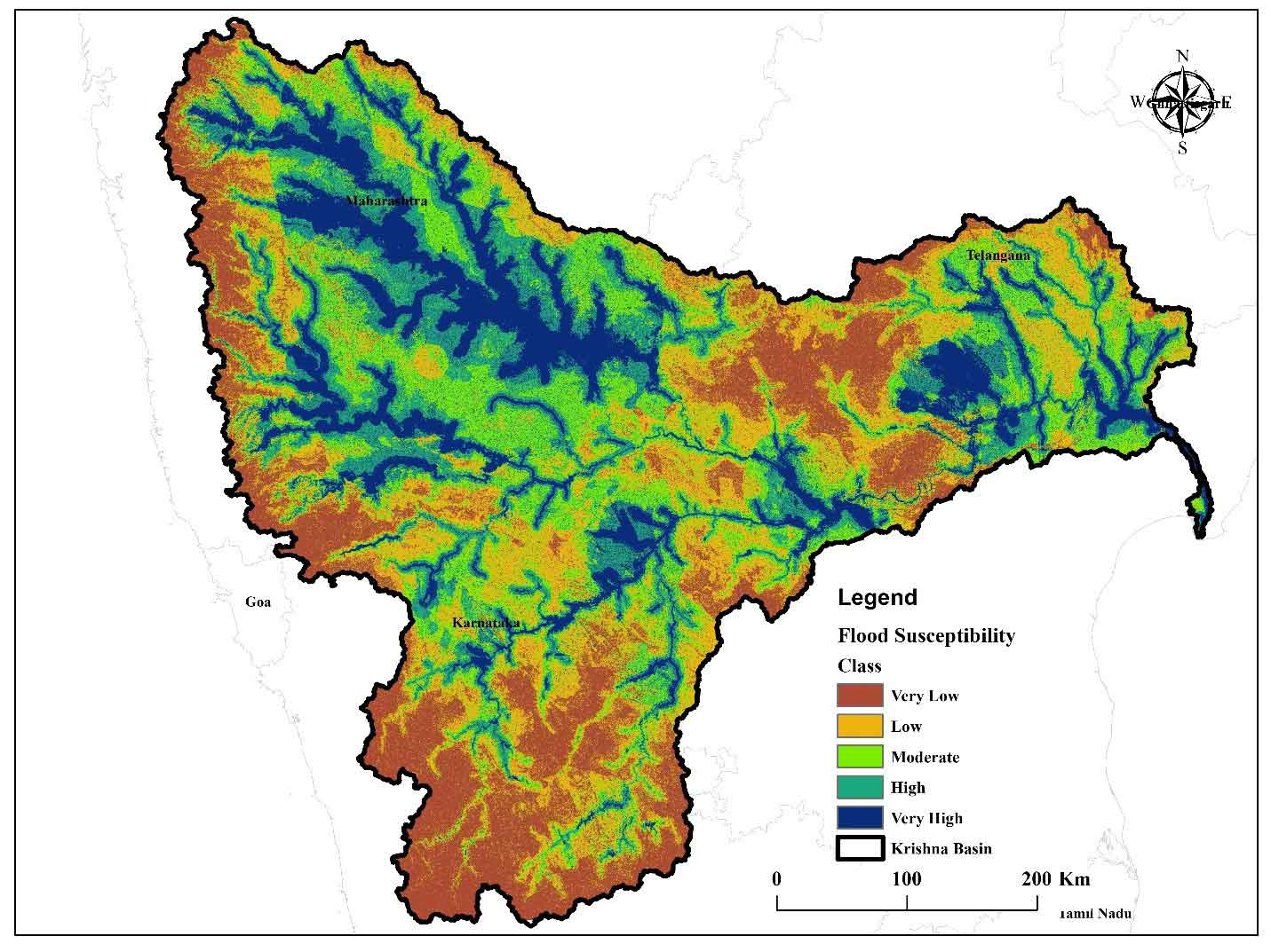
3.3 Flood Susceptibility Mapping
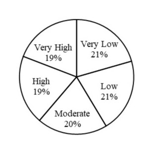
Geomorphic parameters generated in ArcGIS 10.8 were used for flood-susceptibility analysis and for planning measures to manage peak flows during extreme rainfall. The significance of each parameter was evaluated using a pairwise comparison matrix within the AHP-based MCDM framework. The resulting weights were then integrated in a weighted overlay analysis in GIS to generate the flood-susceptibility map. This analytical approach provides a systematic and objective method for assessing flood risk and supporting ground-level planning for mitigation of natural and human-induced hazards. The resultant map was prepared and average scores were calculated and it was categorized into five classes. These classes were re-classified into five flood susceptible zone, i.e. as very low, low, moderate, high and very high (Figure 5) (Arabameri et al., 2020; Doke et al., 2021). Flood vulnerability is strongly controlled by local topography, surface runoff characteristics, and sediment transport processes. Areas classified as very high and high flood-susceptible zones are typically located in low-relief, flat floodplain regions. These areas tend to experience slower surface runoff, higher water accumulation, and increased rates of sediment deposition, which collectively intensify flood impacts (Mahmoud and Gan, 2018). Moderate susceptibility zones occur in areas of intermediate relief, where higher runoff and lower infiltration result in occasional, moderate flooding impacts. Low and very low susceptibility zones characterize steeply sloped regions with rapid runoff, reducing flood risks but limiting groundwater recharge and increasing soil erosion. About 19% of the total area of KRB is highly prone to flooding, most of which falls in the meander belts and floodplain zones of the river. These areas are characterized by gentle to moderate slopes, older floodplains, and a dense drainage network. Factors such as high flow accumulation, heavy rainfall, high runoff, and clay-loam soil further increase flood risk by limiting water absorption.
Additionally, 19% of the area falls within the high flood susceptibility zone, primarily located in the meander belts and floodplains. These regions are characterized by clay–loam soils, which have moderate permeability: they promote groundwater recharge under normal conditions but, during intense rainfall, their limited infiltration rate leads to rapid surface saturation. Combined with gentle slopes, moderate drainage density, and extensive agricultural land use, these factors reduce runoff dispersion and enhance water accumulation, thereby increasing overall flood susceptibility.
The moderate flood susceptibility zone (20%) is characterized by low flow accumulation, moderate drainage density, and greater distance from the main river channel. Areas located farther from the channel typically experience attenuated floodwaters because the depth and velocity of overbank flows decrease with increasing distance from the source (Knighton, 2014). As floodwater disperse across the floodplain, water spreads more thinly, infiltration increases, and the hydraulic impact is reduced (Ward and Robinson, 1975). Consequently, these areas exhibit moderate rather than high flood susceptibility. Factors such as average rainfall, extensive agricultural land, and high percolation capacity due to clay-loam soil contribute to its hydrological response, reducing flood intensity and promoting groundwater recharge.
The low (21%) and very low (21%) flood susceptible zones are mainly found in steep mountainous regions, far from major river channels (Figure 5). These areas exhibit low drainage density, resulting in fewer surface water pathways, which significantly reduces the likelihood of flooding. Despite experiencing high rainfall, the steep topography and dense forest cover caused rapid runoff dispersion and enhance infiltration, effectively minimizing flood risk. Furthermore, the prevalence of natural vegetation helps stabilize slopes and regulate surface water flow, further contributing to reduced flood susceptibility in these zones.
The flood susceptibility maps are presented in a clear and accessible form, allowing users to interpret the results effectively even without specialized technical expertise. However, creating accurate flood maps requires a solid understanding of hydrology, geology, geomorphology, rainfall intensity, flow accumulation, slope, and remote sensing. It has been suggested that focusing on flood-prone and moderately prone areas can help reduce risks to communities, infrastructure, and agriculture (Bagyaraj et al., 2013; Diaz-Alcaide and Martinez-Santos, 2019; Murmu et al., 2019; Andualem and Demeke, 2019; Doke et al., 2021).
AHP is widely used for creating flood susceptibility maps worldwide. This technique helps in detecting areas that are high risk of flooding by analyzing various factors that contribute to flood risk (Kazakis et al., 2015; Hong et al., 2018; Subbarayan and Sivaranjani, 2020; Das and Scaringi, 2021). In addition, highly accurate demarcation of flood prone areas can be achieved using machine learning and real time flood forecasting (Khosravi et al., 2019; Islam et al., 2021; Tran et al., 2025; Wale et al., 2025). The analysis identifies Pune, Shirur, Daund, Phaltan, Baramati, Pandharpur, Solapur, Kolhapur, Sangli, Gokak, Mudhol, Jamkhandi, Bagalkot, Ilkal, Hubballi, Hosapete, Gangavati, Sindhnur, Devarakonda, Gadwal, Itikyal, Nalgonda, Anumula, Guntur, Nandigama, Madhira, Amaravati, Repalle, and Vijayawada are highly flood-prone cities (Table 4 and Figure 7).
However, intense rainfall over the Western Ghat regularly causes rapid inflows into major reservoirs such as Koyna Dam, which has a live storage of approximately 2980 mm³ (Dhumal et al., 2022). During high inflow events, controlled gate releases have surged to over 50,000 cusecs, significantly increasing the flow into the Krishna River (TOI, 2024). When these releases coincide with high river stages and narrow cross-sections downstream, they overwhelm the KRB, as supported by flood-inventory records documenting repeated flood events linked to large dam outflows. This confluence of urban infrastructure limitations, concentrated dam discharges, and seasonal rainfall leads to recurrent flooding, threatening communities and ecosystems in the region. These findings highlight the need for strengthened flood-management strategies, including improved urban drainage design, enhanced reservoir-operation protocols, and sustainable land-use planning. Specific measures such as establishing flood-retention reservoirs, implementing real-time discharge modelling, and expanding early-warning systems can significantly reduce downstream flood impacts. Future research should further examine flood susceptibility for applications in urban planning, disaster preparedness, and rainfall–runoff interactions to support evidence-based flood-risk management.
Table 4. The flood susceptible areas in KRB
|
Sr. No.
|
Basin name
|
High to very high flood susceptible areas
|
|
1
|
Bhima upper sub-basin
|
Pune, Shirur, Dound, Phaltan, Baramati, Pandharpur, and Solapur
|
|
2
|
Krishana upper sub-basin
|
Kolhapur, Sangli, Gokaka, Mudhol, Jamkhandhi, Bagalkot, Iikal
|
|
3
|
Tungbhadra upper basin
|
Hubballi, Hosapate
|
|
4
|
Tungbhadra lower basin
|
Gangavati, Sindhnur
|
|
5
|
Krishana middle sub- basin
|
Devarakonda, Gadwal, Itikyal, Nalgonda, Anumula, Guntur, Nandigama, Madhira, Amravati, Repelle, Vijaywada etc.
|
3.4 Resultant map Validation
Worldwide numerous researchers have adopted different scientific methods for the result validation of geospatial analysis. Among them, the field survey method is considered as the most accurate and useful for direct validation. However, it is costly and time-consuming, so it is not feasible in every research (Das, 2019b).
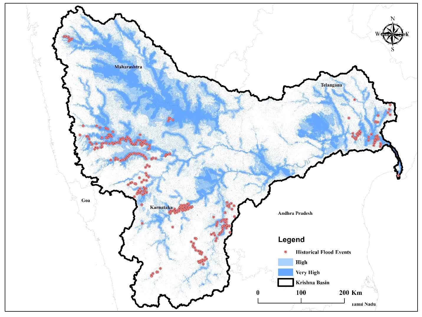
Considering these limitations, validating the Flood Susceptibility map based on historical flood records (Historical Flood Inventory Data) is considered more convenient, effective and scientifically validated (Merz et al., 2007; Wang et al., 2022; Nguyen et al., 2024). The present research has used historical flood spatial data obtained from the Bhuvan Portal from 2009 to 2024 (a website of National Remote Sensing Centre, Government of India). Also, the report published in 2020 by the Water Resources Department of the Government of Maharashtra after a detailed review of the flood situation in the KRB in 2019 has been used as an important reference source for validation. For more scientific confirmation, information about flood-affected areas published in various newspapers has been used. Several mathematical and statistical approaches are commonly employed to validate such studies, including the Success Rate Curve (SRC), Area Under the Curve (AUC), Chi-square test, and flood density analysis (Kayastha et al., 2013).
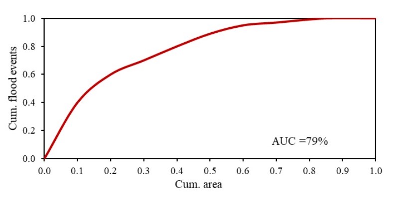
In the present study, flood susceptibility analysis was carried out based on the AHP Model. Point data of 283 different flood-affected locations in the entire KRB has been prepared by the researcher, and this data has been considered as flood inventory data. Based on this data, a scientific method was adopted for validation of the flood susceptibility. The flood susceptibility map was classified into 20 classes. Then, the flood inventory data was overlayed on this map and computed an AUC, through which the accuracy of the map was evaluated.
The bivariate and multivariate statistical methods, frequency ratio models, and machine learning methods are considered scientifically effective for flood analysis; although the machine learning method is complex, it is widely used for high accuracy prediction of locations (Tehrany et al., 2015 a, b; Chen et al., 2017a, b). Compared to the machine learning method, the method adopted in the present research is more relevant and accurate to confirm the flood analysis point of view.
In comparison, the AHP method adopted in the present research is relatively simple, effective and scientifically validated for flood sensitivity analysis. Since the CR value obtained by this method is 0.04 and the AUC value is 79%, it is clear that the results of this research are highly reliable, statistically proven and useful for geographical analysis of flood risk.


 ,
Sanjay Navale 2
,
Sanjay Navale 2