Keywords

Fréchet distribution of maxima , Location and dispersion parameters , Weibull distribution of minima , Moment generating function , Estimation, testing, and point prediction , MLE , Confidence region

1 . Introduction

The general Fréchet distribution for maxima has the form

\(\mathrm{ \Phi _{ \alpha } ( x \vert \lambda , \delta ) = \Phi _{ \alpha } ( \frac{x- \lambda }{ \delta } ) =0 }\)          if        \(\mathrm{x \leq \lambda }\)

\(\mathrm{ \Phi _{ \alpha } ( x ) =exp \{ - ( \frac{x- \lambda }{ \delta } ) ^{- \alpha } \} }\)            if        \(\mathrm{x \geq \lambda ~. }\)

It  is  immediate  that  \(\mathrm{Y= ( \frac{X- \lambda }{ \delta } ) ^{- \alpha } }\) has  the   standard  exponential distribution. Also if \(\mathrm{ \lambda = \lambda _{0} }\) is known (it can be taken as zero, for convenience, by subtraction) \(\mathrm{\tilde{Y}=log ( X- \lambda _{0} ) }\)has a Gumbel distribution of maxima with location and dispersion parameters log \(\mathrm{\delta}\) and \(\mathrm{1/\alpha}\). Thus theory for Gumbel distribution can be applied, and the maximum likelihood estimators of \(\mathrm{\left( \lambda , \delta \right) }\) \(\mathrm{\left( if~ \lambda _{0}=0 \right) }\) are given by the equations.

\(\mathrm{ \frac{n}{ \hat{\alpha} }- \sum _{1}^{n}log\,x_{i}+n\frac{ \sum _{1}^{n}x_{i}^{- \hat{\alpha} }log\,x_{i}}{ \sum _{1}^{n}x_{i}^{- \hat{\alpha} }}=0 }\)

\(\mathrm{ \hat{\delta }^ \hat{\alpha }=\frac{n}{ \sum _{1}^{n}x_{i}^{- \hat{\alpha} }} }\) . 

The solution of the first equation needs an initial seed which can be obtained using the fact that \(\mathrm{ \{ log\,x_{i} \} }\) has dispersion parameter \(\mathrm{1/\alpha}\) of a general Gumbel distribution among other ways.

The random pair \(\mathrm{( \hat{\delta }, \hat{\alpha } ) }\) is asymptotically normal with mean values \(\delta\) and \(\alpha\), variances \({ \delta ^{2}}/({n}~ \alpha ^{2})\cdot [ 1+{6}/{ \pi ^{2}} \left( 1- \gamma \right) ^{2} ] \), and \(6~ \alpha ^{2}/(n~ \pi ^{2}) \) , covariance \(\frac{6 \left( 1- \gamma \right) \delta }{n~ \pi ^{2}} \) and correlation coefficient   \(\rho =- ( 1+\frac{ \pi ^{2}}{6 \left( 1- \gamma \right) ^{2}} ) ^{{-1}/{2}}=.31307.\)

This should be expected from the formulae given before for the Gumbel distribution.

The asymptotic confidence region with a significance level \(\mathrm{ \alpha ’ }\)is given by

\(\mathrm{ \alpha ^{2} ( \hat{\delta} - \delta ) ^{2}+2 ( 1- \gamma ) \delta ( \hat{\delta}- \delta ) ( \hat{\alpha }- \alpha ) + ( \frac{ \pi ^{2}}{6}+ ( 1- \gamma ) ^{2} ) \delta ^{2} ( \frac{ \hat{\alpha } - \alpha }{ \alpha } ) ^{2} \leq -2\,log\, \alpha ’\cdot \delta ^{2} }\)

where, to avoid big changes of notation, the \(\mathrm{ \alpha' }\) in the RHS of the inequality is the significance level. The substitution of \(\mathrm{ \alpha }\) and \(\mathrm{ \delta }\) by \(\mathrm{ \hat{\alpha} }\) and \(\mathrm{ \hat{\delta} }\) except in the differences \(\mathrm{ (\hat{\alpha}-\alpha) }\)  and \(\mathrm{ (\hat{\delta}-\delta) }\) gives a part of an ellipsis in the quadrant \(\mathrm{( \alpha >0, \delta >0 ) }\) . From the same result we can make the rule for asymptotic tests of hypotheses.

The estimator of the quantile \(\chi _{X,p}= \delta / ( -log~p ) ^{1/ \alpha }\) is evidently taken as \(\hat\chi _{X,p}= \hat\delta /( -log~p ) ^{1/\hat \alpha }\) , it is asymptotically normal with mean value \(\chi _{X,p} \) and variance

\(( -\,log\,p ) ^{-2/\hat{\alpha }} [ 1+\frac{6}{ \pi ^{2}} ( 1- \gamma -log ( -\,log\,⁡p ) ) ^{2} ] { \delta ^{2}}/{n}\, \alpha ^{2} \)

or, equivalently from the asymptotic point of view,

\(( -\,log\,p ) ^{-2/\hat{\alpha }} [ 1+\frac{6}{ \pi ^{2}} ( 1- \gamma -log ( -\,log\,⁡p ) ) ^{2} ] { \hat\delta ^{2}}/{n}\, \hat\alpha ^{2} \) .

As the mean value of the maximum of the next \(m\) observations is \(m^{-1⁄ \alpha }\, \Gamma ( 1-/{1}/{ \alpha } ) \delta \left( if~ \alpha >1 \right) \) we can take as estimator \(m^{-1⁄ \hat{\alpha} ~} \Gamma ( 1-{1}/{ \hat{\alpha} } ) \hat{\delta} \); this estimator is asymptotically normal with the same mean value referred to and variance

\({\frac{ \Gamma ^{2} ( 1-/{1}/{ \alpha } ) }{m^{/{2}/{ \alpha }}\cdot\, \alpha ^{2}~n} [ 1+\frac{6}{ \pi ^{2}}~ ( \gamma +\frac{ \Gamma ^{’} ( 1-{1}/{ \alpha } ) }{ \Gamma ( {1}/{ \alpha } ) } ) ^{2} ]} \).

Equivalently, from the asymptotic point of view, we can substitute in the variance \(\mathrm{ \delta }\) and \(\mathrm{ \alpha }\) by \(\mathrm{ \hat{\delta} }\) and \(\mathrm{ \hat{\alpha} }\) . The asymptotic variance exists only if \(\mathrm{ \alpha >2}\) , as it will be seen shortly.

It is worth noting that if \(\mathrm{ X}\) has a Fréchet distribution of maxima with \(\mathrm{ \lambda = \lambda _{0}=0 }\) and dispersion and location parameters \(\mathrm{ \delta }\) and \(\mathrm{ \alpha }\), then \(\mathrm{ 1/X }\)   has a Weibull distribution of minima (to be studied in the next chapter) with, also, \(\mathrm{ \lambda = \lambda _{0}=0 }\), and dispersion and shape parameters \(\mathrm{ 1/\delta }\) and \(\mathrm{ \alpha }\); so the techniques for the Fréchet distribution of maxima and Weibull distribution of minima can be exchanged.

As far as applications are concerned, as said before, they have been done for largest waves and floods of rivers.

2 . Characteristics of the Fréchet distribution

From the Fréchet distribution

\(\mathrm{ \Phi _{ \alpha } ( \frac{x- \lambda }{ \delta } ) =0 }\)                                if   \(\mathrm{ x \leq \lambda }\)

\(\mathrm{ \Phi _{ \alpha } ( x ) =exp⁡ \{ - ( \frac{x- \lambda }{ \delta } ) ^{- \alpha } \} }\)             if   \(\mathrm{ x \geq \lambda }\)

we can get the usual coefficients if they exist. So we will compute them for the reduced random variable \(\mathrm{ Z= ( X- \lambda ) / \delta }\), the transfer to the general case being obvious as seen in the previous chapter.

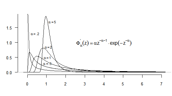
The graph of the probability densities \(\mathrm{ \Phi _{ \alpha }^{’} ( z ) ( z \geq 0 ) }\) for different values of \(\mathrm{\alpha>0}\)  are given in figure 6.1.

Figure 6.1 Reduced Fréchet densities (for maxima)

For \(\mathrm{ \Phi _{ \alpha }^{’} ( z ) = \alpha\ z^{-1- \alpha } ( exp ( -z^{- \alpha } ) ) }\), the mode is \(\mathrm{\mu ’= ( \frac{ \alpha }{1+ \alpha } ) ^{1/ \alpha } }\) , the median \(\mathrm{\mu = \left( log\,2 \right) ^{-1/ \alpha } }\) , and the quantile   \(\mathrm{\chi _{p}= \left( -log\,p \right) ^{-1/ \alpha } }\) with \(\mathrm{\chi _{1/e}=1 }\) .

As regards moments, they exist only if \(\mathrm{ r< \alpha }\) , and have the expression \(\mathrm{{ \mu'}_{r}= \Gamma ( 1-r/ \alpha ) }\) . Consequently, we have as mean value \(\mathrm{ \mu = \Gamma ( 1-r/ \alpha ) }\) if \(\mathrm{1<\alpha}\) and as variance \(\mathrm{ \sigma ^{2}= \Gamma ( 1-2/ \alpha) - \Gamma ^{2} ( 1-1/ \alpha )~ if~2< \alpha }\), the corresponding values for \(\mathrm{ X= \lambda + \delta \,z }\) being obvious. The computation of \(\mathrm{ \beta _{1} }\) and  \(\mathrm{ \beta _{2} }\), which depend on \(\mathrm{\alpha}\), is left as an exercise. Notice that the negative order moments always exist.

An important point to recall is that if \(\mathrm{Z}\) has the distribution function \(\mathrm{\Phi _{ \alpha } ( z ) }\) then \(\mathrm{ Prob\{ { \alpha ( Z-1 )\leq\,y \}} = \Phi _{ \alpha } ( 1+\frac{y}{ \alpha } ) \rightarrow \Lambda ( y ) ~as~ \alpha \rightarrow \infty }\). This means that for large \(\mathrm{\alpha}\) we can use the Gumbel distribution as an approximation to the Fréchet distribution; see the exercises related to approximation of \(\mathrm{ \Phi _{ \alpha } ( 1+y/ \alpha ) ~by~ \Lambda ( z ) }\).  

The moment generating function of \(\mathrm{Z}\) has no explicit expression, but that of \(\mathrm{log\,Z}\) is \(\mathrm{ M ( e^{ \theta ~log~Z}\, t) =M ( Z^{ \theta } ) = \Gamma ( 1- \theta / \alpha ) }\), defined only for \(\mathrm{\theta < \alpha }\), as could be expected from the moment, \(\mathrm{M ( Z^{ \theta } ) }\) giving the cumulants associated with the moments.

3 . Estimation, testing, and point prediction

Let us now consider the statistical decision for the 3-parameters case. The likelihood being

\(\mathrm{L ( \lambda , \delta , \alpha \vert x_{i} ) =0 }\)    if     \(\mathrm{min ( x_{1},\dots,x_{n} ) \leq \lambda }\)

\(\mathrm{L \left( \lambda , \delta , \alpha \vert x_{i} \right) =\frac{ \alpha ^{n}~ \delta ^{n~ \alpha }} {{\mathrm{\begin{matrix} n \\ \pi \\ 1 \end{matrix}}}{{ \left( x_{i}- \lambda \right) ^{ \alpha +1}}}}~exp⁡ \{ - \delta ^{ \alpha } \sum _{1}^{n} \left( x_{i}- \lambda \right) ^{- \alpha } }\}\)                     if   

\(\mathrm{min ( x_{1},\dots,x_{n} ) > \lambda ,}\)

the maximum likelihood estimators are given by

\(\mathrm{\hat{\delta}^ {\hat{\alpha }}=\frac{n}{ \sum _{1}^{n} ( x_{i}- \hat{\lambda } ) ^{- \hat{\alpha} }} }\)

\(\mathrm{\frac{ ( \hat{\alpha} +1 ) }{ \hat{\alpha} } \sum _{1}^{n} ( x_{i}- \hat{\lambda} ) ^{-1}=\frac{n \sum _{1}^{n} ( x_{i}- \hat{\lambda} ) ^{-\hat{\alpha} -1}}{ \sum _{1}^{n} ( x_{i}- \hat{\lambda} ) ^{- \hat{\alpha} }} }\)

\(\mathrm{\frac{1}{n} \sum _{1}^{n}log ( x_{i}- \hat{\lambda} ) -\frac{1}{ \hat{\alpha} }=\frac{ \sum _{1}^{n} ( x_{i}- \hat{\lambda}) ^{- \hat{\alpha} }log⁡ ( x_{i}- \hat{\lambda} ) }{ \sum _{1}^{n} ( x_{i}- \hat{\lambda} ) ^{- \hat{\alpha} }} }\)

For this system we have to solve, first, the last two equations and immediately compute \(\mathrm{ \hat{\delta }}\) .

Note that the solutions must be admissible, i.e., they must satisfy \(\mathrm{ \hat{\lambda } \leq min ( x_{1},\cdots,x_{n} ) , \hat{\alpha }>0 }\) and \(\mathrm{ \hat{\delta }>0}\) being obvious from the relations defining them. To obtain a first approximation to \(\mathrm{( \hat{\lambda }, \hat{\alpha } ) }\) we can follow Gumbel (1965). Denoting by \(\mathrm{ min \{ x_{i} \} , }\) \(\mathrm{ med \{ x_{i} \} , }\) and \(\mathrm{ max \{ x_{i} \} , }\) the minimum, the median and the maximum of the sample, we have the first approximations \(\mathrm{( \hat{\lambda }_1, \hat{\alpha }_1 ) }\)

\(\mathrm{ Q_{n}=\frac{max\{ { x_{i}\} } -med \{{ x_{i}\} } }{med\{ { x_{i}\} } -min \{{ x_{i}\} } }=Q ( \frac{1}{ \hat{\alpha} _{1}},n ) }\)

\(\mathrm{ \hat{\lambda }_{1}=\frac{n^{1/ \hat{\alpha }_{1}}med~ { \{x_{i}\} } -max { \{x_{i}\} } }{n^{1/ \hat{\alpha }_{1}}-1} }\).

Gumbel (1965) gives a table of the function \(\mathrm{ Q ( 1/ \alpha ,n ) }\) (\(\mathrm{ 1/ \alpha }\) there being called \(\mathrm{ \lambda }\) ) for values of \(\mathrm{ \alpha >1}\) . The statistic \(\mathrm{ Q_n}\) was considered as a tool for the quick statistical choice of extreme models in Chapter 4.

We will now compute the asymptotic sampling characteristics of the maximum likelihood estimators \(\mathrm{( \hat{\lambda },\hat{\delta}, \hat{\alpha } ) }\).

The variance-covariance matrix is

\(\mathrm{ \frac{1}{n} \cdot \begin{bmatrix} \frac{(\alpha+1)^2\Gamma(1+2/\alpha)}{\delta^2} & \frac{\alpha(\alpha+1)\Gamma(1+1/\alpha)}{\delta^2} & \frac{(\alpha+1)[\Gamma(1+1/\alpha)+\Gamma'(1+1/\alpha)]}{\alpha\delta} \\[0.3em] \frac{\alpha(\alpha+1)\Gamma(1+1/\alpha)}{\delta^2} & \frac{\alpha^2}{\delta^2} & \frac{1-\gamma}{\delta} \\[0.3em] \frac{(\alpha+1)[\Gamma(1+1/\alpha)+\Gamma'(1+1/\alpha)] }{\alpha\delta} & \frac{1-\gamma}{\delta} & \frac{1}{\alpha^2}{(\frac{\pi^2}{6}+(1-\gamma)^2)} \end{bmatrix}}^{-1}\)

as given by Tiago de Oliveira (1973).

The asymptotic confidence region with level of significance \(\mathrm{ \alpha ’ }\)  is given by

\(\frac{ \left( \alpha +1 \right) ^{2} \Gamma \left( 1+{2}/{ \alpha } \right) }{ \delta ^{2}}( \hat{ \lambda} - \lambda ) ^{2}+\frac{ \alpha ^{2}}{ \delta ^{2}} ( \hat{ \delta }- \delta ) ^{2}\) \(+\frac{1}{ \alpha ^{2}} ( \frac{ \pi ^{2}}{6}+ ( 1- \gamma ) ^{2} ) ( \hat{\alpha } - \alpha ) ^{2}\)\( +\frac{2\, \alpha( \alpha +1 ) ~ \Gamma ( 1+{1}/{ \alpha } ) }{ {\delta} {^{2}}} \)\(( \hat{ \lambda} - \lambda ) ( \hat{ \delta } - \delta )\)

\( +\frac{2 ( \alpha +1 ) \, [ \Gamma ( 1+{1}/{ \alpha } ) + \Gamma ^{’} ( 1+{1}/{ \alpha } ) ] }{ \alpha\, \delta } ( \hat{ \lambda} - \lambda ) (\hat{\alpha } - \alpha ) \)\(\mathrm{+\frac{2 ( 1- \gamma ) }{ \delta } ( \hat{\delta} - \delta ) ( \hat{\alpha }- \alpha ) \leq \frac{ \chi _{3}^{2} ( \alpha ’ ) }{n} }\)

where   \(\mathrm{\chi _{3}^{2} \left( \alpha ’ \right) }\)  is the point \(\mathrm{ \alpha ’ }\) for a \(\mathrm{ \chi ^{2} }\) with 3 degrees of freedom.

The usual tests of hypotheses can be made using this asymptotic confidence region.

The estimator of the quantile \(\chi _{X,p}= \lambda + \left( -\,log\,p \right) ^{-1/ \alpha }\, \delta \)  is \(\hat{\chi }_{X,p}= \hat{\lambda }+ \left( -\,log\,p \right) ^{-1/ \hat{\alpha }} \hat{\delta } \). It is asymptotically normal with mean value \(\chi _{X,p} \) and asymptotic variance

\(V ( \hat{\lambda} ) + ( -log\,p ) ^{-{2}/{ \alpha }}\,V ( \hat{ \delta} ) +\frac{ \delta ^{2}}{ \alpha ^{4}} \left( -log\,p \right) ^{-{2}/{ \alpha }} \left( log \left( -\,log⁡\,p \right) \right) ^{2}\,V ( \hat{\alpha} ) \)\(+2\, \left( -log\,p \right) ^{-{1}/{ \alpha }}\,C ( \hat{\lambda} , \hat{\delta} ) +\frac{2\, \delta \, \left( -log\,p \right) ^{-1- \alpha }\,log\, \left( -log\,p \right) }{ \alpha ^{2}}\,C ( \hat{\lambda} , \hat{\alpha} ) \)\(+\frac{2\, \delta }{ \alpha ^{2}} ( -\,log\,p ) ^{-2/ \alpha }\,log ( -log\,p ) \,C ( \hat{\delta} , \hat{\alpha} )\).

The least squares predictor of the mean value of the maximum of the next \(m\) observations \(\lambda +m^{-1/ \alpha }\, \Gamma \left( 1-{1}/{ \alpha } \right) \delta \) is given by \(\hat{\lambda }+m^{-1/ \hat{\alpha} }\, \Gamma ( 1-{1}/{ \hat{\alpha} } ) \hat{\delta} \)   \(\left( if~1< \alpha \right) \) and its asymptotic variance is

\(V ( \hat{\lambda} ) +m^{-2/ \alpha }~ \Gamma ^{2} ( 1-{1}/{ \alpha }) ~V( \hat{ \delta}) +\frac{ \delta ^{2}m^{-2/ \alpha }}{ \alpha ^{4}} [ \Gamma ^{’} ( 1-{1}/{ \alpha })\)\(+ ( log\,m ) \Gamma ( 1-{1}/{ \alpha } ) ] ^{2}~V( \hat{ \alpha} ) +2\,m^{-1/ \alpha }~ \Gamma ( 1-{1}/{ \alpha } ) ~C( \hat{\lambda} , \hat{ \delta})\)

\(+\frac{2\,m^{-1/ \alpha }}{ \alpha ^{2}}[ \Gamma ^{’}( 1-{1}/{ \alpha } ) +log\,m ) \Gamma ( 1-{1}/{ \alpha } ) ] ~C ( \hat{\lambda}, \hat{ \alpha} )\)\( +\frac{2 \,m^{-{2}/{ \alpha }}\, \Gamma( 1-{1}/{ \alpha } ) \delta }{ \alpha ^{2}}~ [ \Gamma ( 1-{1}/{ \alpha }) +log\,m )\, \Gamma ( 1-{1}/{ \alpha } )] ~C ( \hat{ \delta} ,\hat{ \alpha} ) \)

\( (if~2< \alpha ) \); the mean-square error of the predictor is obtained by adding \(\mathrm{ V ( X ) = [ \Gamma \left( 1-{2}/{ \alpha } \right) - \Gamma ^{2} ( 1-{1}/{ \alpha } ) ] \delta ^{2} }\).

The computation of the asymptotic variances is easily made from the formulae given, substituting \(\mathrm{( \lambda , \delta , \alpha ) }\) by \(\mathrm{ ( \hat{\lambda} , \hat{\delta} , \hat{\alpha} ) }\).

4 . Overpassing probability for a level

The probability of overpassing a level \(a ( > \lambda )\) is

\({\mathrm{P} ( a) ={\mathrm{P}} ( a \vert \lambda , \delta , \alpha ) ={\mathrm{Prob}}{\{ \mathrm{X}>a\}} =1- \Phi _{ \alpha } ( \frac{a- \lambda }{ \delta }) }\)

which is estimated by substituting \(\mathrm{( \lambda , \delta , \alpha ) }\) by its maximum likelihood estimators \(\mathrm{ ( \hat{\lambda} , \hat{\delta} , \hat{\alpha} ) }\), already given. Then

\({\mathrm{\sqrt[]{n}\, ( \hat{P}} ( a ) -\mathrm{P} ( a ) )}\)

is asymptotically equivalent, by the \(\mathrm{ \delta }\) -method, to its linearized form

\({\mathrm{ \sqrt[]{n}}\, [ ( \hat{\lambda} - \lambda ) \frac{ \partial \,{\mathrm{P}} \left( a \right) }{ \partial \lambda }+ ( \hat{ \delta} - \delta ) \frac{ \partial \,{\mathrm{P}} \left( a \right) }{ \partial \delta }+ ( \hat{ \alpha} - \alpha ) \frac{ \partial \,{\mathrm{P}} \left( a \right) }{ \partial \alpha } ] = }\)

\({\mathrm{ =\sqrt[]{n}} \, ( 1-{\mathrm{P}} \left( a \right) ) ( -{\mathrm{log}}\,( 1-{\mathrm{P}}( a ) ) \{ \alpha\, \frac{ \hat{\lambda }- \lambda }{a- \lambda }+ \alpha \frac{\hat{\delta} - \delta }{ \delta }-{\mathrm{log}}\,\frac{a- \lambda }{ \delta }\, ( \hat{\alpha }- \alpha ) \} , }\)

and so \({\mathrm{\sqrt[]{n}} \,\{\hat{\mathrm{P}} ( a ) -{\mathrm{P}} ( a ) \}}\) is asymptotically normal with mean value zero and variance

\({\mathrm{{ V}} ( a \vert \lambda , \delta , \alpha) ={\mathrm{V}} ( a ) = ( 1-{\mathrm{P}} ( a ) ) ^{2}\,( {\mathrm{log}}\, ( 1-{\mathrm{P}} ( a ) ) ^{2}\, \times }\)

\({\mathrm{\begin{array}{c}\\ {\mathrm{\lim n}}\\{\mathrm{x \to {n}}} \end{array} } \{ \alpha ^{2}\frac{\mathrm{{V}} ( \hat{\lambda} ) }{ ( a- \lambda ) ^{2}}+\frac{ \alpha ^{2}{\mathrm{V}} ( \hat{ \delta} ) }{ \delta ^{2}}+ ( {\mathrm{log\frac{a- \lambda }{ \delta } ) ^{2}}}\,{\mathrm{V}} ( \hat{ \alpha} ) + }\)

\({\mathrm{ +2}\,\frac{ \alpha ^{2}}{ ( a- \lambda ) \delta }\,{\mathrm{C}} ( \hat{ \lambda} ,\, \hat{\delta } ) -2\, \alpha \frac{\mathrm{log} \left( { \left( a- \lambda \right) }/{ \delta } \right) }{a- \lambda }\,{\mathrm{C}} ( \hat{\lambda} , \hat{\alpha} ) -2\,\frac{ \alpha }{ \delta }\,{\mathrm{log}}\,\frac{a- \lambda }{ \delta }\,{\mathrm{C}} ( \hat{ \delta} ,\hat{ \alpha} ) \} }\).

Substituting \(\mathrm{ ( \lambda , \delta , \alpha ) }\) by their maximum likelihood estimators \(\mathrm{( \hat{\lambda} , \hat{\delta} , \hat{\alpha} ) }\), we also get \({\mathrm{\hat{V} ( a ) =V ( a \vert \hat{\lambda} , \hat{\delta} , \hat{\alpha} )} \sim {\mathrm{V}} ( a)}\) and, thus \({\mathrm{ \sqrt[]{n}}~\frac{\hat{\mathrm{P}} \left( a \right) -{\mathrm{P}} \left( a \right) }{\sqrt[]{\hat{\mathrm{V} }\left( a \right) }} }\) is asymptotically standard normal, and so the one-sided asymptotic confidence interval with significance level \(\mathrm{ \alpha' }\) for \({\mathrm{ P}(a) }\) is

\({\mathrm{ 0 \leq P} ( a ) {\mathrm{\leq \hat{P}}} ( a ) +\frac{ \lambda _{ \alpha ’}}{\mathrm{{\sqrt[]{n}}}}\sqrt[]{\mathrm{\hat{V}} ( a ) } }\)

as before.

When \(\mathrm{ ​​\lambda }\) is known ( \(\mathrm{ 0 }\) for convenience) we have \({\mathrm{ P} ( a ) ={\mathrm{P}} ( a \vert \delta , \alpha ) =1- \Phi _{ \alpha } ( a/ \delta ) }\) , which corresponds to the case of some rivers and wave heights. Then the variance-covariance matrix of the maximum likelihood estimators \(\mathrm{ ( \hat{\delta} , \hat{\alpha} ) }\) is

\(\mathrm{ \frac{1}{n} \begin{bmatrix} \frac{\alpha^2}{\delta^2} & \frac{1-\gamma}{\delta} \\[0.3em]\frac{1-\gamma}{\delta}& \frac{1}{\alpha^2}(\frac{\pi^2}{6}+(1-\gamma)^2) \\[0.3em] \end{bmatrix}^{-1}}\mathrm{ =\frac{1}{n} \begin{bmatrix} \frac{\delta^2}{\alpha^2}(1+\frac{6}{\pi^2}(1-\gamma)^2) & \frac{6(1-\gamma)}{\pi^2}\delta \\[0.3em]\frac{6(1-\gamma)}{\pi^2}\delta& \frac{6\,\alpha^2}{\pi^2} \\[0.3em] \end{bmatrix}}\)

and thus with \({\mathrm{ \hat{P}} ( a ) ={{\mathrm{P ( a \vert \hat{\delta} , \hat{\alpha} ) }}}}\) , \({\mathrm{\sqrt[]{n}} \,\,({\mathrm{\hat{P}}} ( a ) -{\mathrm{P}} ( a )) }\)is asymptotically equivalent to

\({\mathrm{ \sqrt[]{n}\, [ ( \hat{ \delta} - \delta )} \frac{ \partial \,{\mathrm{P}} ( a ) }{ \partial \, \delta }+ ( \hat{ \alpha} - \alpha ) \frac{ \partial \,{\mathrm{P}} ( a ) }{ \partial \, \alpha } ] = }\)

\({\mathrm{ =\sqrt[]{n}}\, \left( 1-{\mathrm{P}} \left( a \right) \right) \, \left( {\mathrm{log}} \left( 1-{\mathrm{P}} \left( a \right) \right) \right) \, [ \alpha\, \frac{\hat{ \delta} - \delta }{ \delta }+{\mathrm{log}}\,\frac{ \delta }{a}- \left( \hat{ \alpha} - \alpha \right) ] }\) .

Thus \({\mathrm{\sqrt[]{n}} \,\,({\mathrm{\hat{P}}} ( a ) -{\mathrm{P}} ( a )) }\) is asymptotically normal with zero mean value and variance

\({\mathrm{ V} ( a ) \sim ( 1-{\mathrm{P}} ( a ) ) ^{2}\, ( {\mathrm{log}}\,( 1-{\mathrm{P}} ( a ) )) ^{2}\, \{ 1- \gamma + \alpha \,{\mathrm{log}}\,\frac{ \delta }{a} \} }\);

\({\mathrm{ \hat{V}}(a) }\) , as before, denotes \({\mathrm{ V}(a) }\) when \(\mathrm{ ( \delta , \alpha ) }\) are substituted by \(\mathrm{ ( \hat{\delta} , \hat{\alpha} ) }\), and from the practical point of view, for large \(\mathrm{ n }\), we can use the fact that

\(\sqrt[]{n}~\frac{\hat{P} \left( a \right) -P \left( a \right) }{\sqrt[]{\hat{V} \left( a \right) }} \) is asymptotically standard normal. The one-sided asymptotic confidence interval for the probability of overpassing the level \(a\) is

\(0 \leq P ( a ) \leq \hat{P} ( a ) +\frac{ \lambda _{ \alpha ’}}{\sqrt[]{n}}\sqrt[]{\hat{V}( \alpha ) } \)

with significance level \(\alpha'\) .

5 . A worked example

Let us use the data given in the worked example for the Gumbel distribution, but for 24h duration, which is said to verify the Fréchet distribution.

We then get \(\mathrm{ \hat{\lambda} =-10.615183 }\) , \(\mathrm{ \hat{\delta }=38.998362 }\) , and \(\mathrm{ \hat{\alpha} =4.318996 }\) . The Kolmogoroff-Smirnov statistic is \(\mathrm{ \hat{K}S_{n}={\mathrm{\sup_{x }}} \vert S_{n} ( x ) - \Phi _{\hat{ \alpha} } ( ( x- \hat{\lambda} ) / \hat{\delta} ) \vert =0.0681721 }\) and as \(\mathrm{ n=35 }\) we have \(\mathrm{ \sqrt[]{n}~\hat{K}S_{n}=0.40331 }\) , accepting thus the Fréchet model.

Tables

Figures

References