Keywords

Weibull distribution , Minima , Point prediction , Time-to-failure

1 . Introduction

The Weibull distribution for minima is one of the asymptotic distributions for minima when the initial distribution has a left-end point (recall that the other possible asymptotic distribution is the Gumbel distribution for minima). Thus any Weibull random variable (for minima) has a finite location parameter \(\mathrm{ \lambda }\)  (a threshold) and it takes the form

\(\mathrm{ W_{ \alpha }( x \vert \lambda , \delta) =W_{ \alpha } ( \left( {x- \lambda)/ }{ \delta } \right) =1-exp \{ - \left( \frac{x- \lambda }{ \delta } \right) ^{ \alpha } \} }\)    for    \(\mathrm{ ~x \geq \lambda }\)

\(\mathrm{ W_{ \alpha } \left( x \vert \lambda , \delta \right) =W_{ \alpha } \left( \left( x- \lambda \right) / \delta \right) =0 }\)                                for     \(\mathrm{ ~x \leq \lambda . }\)

For \(\mathrm{ \alpha =1 }\) , we have the exponential distribution and for \(\mathrm{ \alpha =2 }\)  we have the Rayleigh distribution important in delay-times and Oceanography, respectively. Evidently \(\mathrm{ W_{ \alpha } \left( z \right) =1- \Psi _{ \alpha } \left( -z \right) }\).

It is immediate that \(\mathrm{ Y= \left( \left( X- \lambda \right) / \delta \right) ^{ \alpha } }\)  has the standard exponential distribution. Also if  \(\mathrm{ \lambda = \lambda _{0} }\) is known (it can be taken as zero, for convenience, by subtraction) \(\mathrm{ Y=-log \left( X- \lambda _{0} \right) }\) has a Gumbel distribution for maxima with the location and dispersion parameters \(\mathrm{ -~log~ \delta }\)  and \(\mathrm{1/ \alpha }\). Thus the theory for Gumbel distribution can be applied and the maximum likelihood estimators are  \(\mathrm{\left( if~ \lambda _{0}=0 \right) }\)

\(\mathrm{\frac{n}{ \hat{\alpha} }- \sum _{1}^{n}log~x_{i}-n~\frac{ \sum _{1}^{n}~x_{i}^{ \hat{\alpha} }.~log~x_{i}}{ \sum _{1}^{n}~x_{i}^{ \hat{\alpha} }}=0 }\)

\(\mathrm{\hat{\delta} =\frac{1}{n} \sum _{1}^{n}x_{i}^{\hat{ \alpha} }. }\)

The solution of the first equation needs an initial seed which can be obtained either using the fact that \(\mathrm{\{ -~log~x_{i} ) }\)  has a general Gumbel distribution where \(\mathrm{1/ {X} }\) is the dispersion parameter among other ways.

The random pair \(( \hat{\delta} , \hat{\alpha } )\)  has a binormal asymptotic behaviour with mean values \(\left( \delta , \alpha \right)\) ,variances \({ ( 1+\frac{6}{ \pi ^{2}} ( 1- \gamma ) ^{2} ) \delta ^{2}}/{n \alpha ^{2}and}~6~{ \alpha ^{2}}/{n}~ \pi ^{2} \), covariance \(\frac{6 \left( 1- \gamma \right) \delta }{n~ \pi ^{2}} \), and correlation coefficient \(\rho = (1+\frac{ \pi ^{2}}{6 ( 1- \gamma ) ^{2}}) ^{-{1}/{2}}=.31307 \).

The confidence intervals; tests, estimators of quantiles, predictors, etc., can be dealt with by the usual techniques, as done before in previous chapters.

Weibull (1939) gave an empirical derivation of this distribution in an analysis of dynamic breaking strengths by requiring only that is should meet certain practical criteria. That paper and other related papers by Weibull dealing with the modelling of failure (or survival) data seem to have found a large audience chiefly among those concerned with reliability analysis. The use of the Weibull distribution as a model for “time-to-failure” has thus been widespread. It arises naturally also in the analysis of droughts, in Oceanography, in Survival Analysis; see, for instance, Gumbel (1954).

The Weibull distribution for maxima has been used to model maximum temperatures, maximum wind speeds and maximum earthquake magnitudes; see Jenkinson (1955) and Yegulalp and Kuo (1974).

Other methods of estimation, as the ones given for the Gumbel distribution, can be used by the reduction to   \(\mathrm{ y_{i}=-log~x_{i} }\) .

Recall that if \(\mathrm{ X }\)  has a Fréchet distribution with dispersion and shape parameters \(\mathrm{ \delta }\)  and \(\mathrm{ \alpha }\) , respectively, then \(\mathrm{1/ \alpha }\)  has a two-parameter Weibull distribution with shape parameter \(\mathrm{ \alpha }\)   and dispersion parameter \(\mathrm{ \delta^{-1} }\) . Thus, when data have not been censored, estimation procedures that have been derived for the two-parameter Fréchet distribution can be used to estimate parameters of the Weibull distribution by simply taking reciprocals of the observed values or directly when appropriate.

Methods applicable for Weibull censoring on the right will be appropriate for censoring Fréchet data sets on the left, i.e., the smallest data values, etc.

For these censorings, and for obtaining best invariant estimators of \(\mathrm{ -log~ \delta }\)  and \(\mathrm{1/ \alpha }\)  among those which are linear in the Gumbel order statistics (logarithms of the Weibull order statistics in reverse order), weights have been calculated and tabulated by Laue (1974) for  \(\mathrm{ n=1 ( 1 ) 25,~r=2 ( 1 ) n }\) . For zero censoring they are equal to the weights calculated and tabulated by Mann (1967) for best linearly invariant estimation from the smallest \(\mathrm{ r \leq n }\)   Gumbel order statistics.

From best linearly invariant estimators of \(\mathrm{ -~log~ \delta }\)  and \(\mathrm{ \alpha^{-1} }\)  one can obtain estimators of the location and dispersion parameters and best linearly estimators of any quantile of the distribution. Invariant estimators and maximum likelihood equations yield estimators of \(\mathrm{ \alpha^{-1} }\)  and \(\mathrm{ -~log~ \delta }\)  that tend to be very nearly equal in value, ant the constants in the variance-covariance matrix of the best linearly unbiased estimators can be used effectively to remove the bias from maximum likelihood estimators if approximate unbiased estimators are desired. All these types of estimators are asymptotically unbiased, asymptotically efficient and asymptotically normal.

2 . Characteristics of the Weibull distribution

From the definition of the distribution function

\(\mathrm{ W_{ \alpha } ( x \vert \lambda , \delta ) =1- \Psi _{ \alpha } ( -x \vert \lambda, \delta ) }\)

we can get, when they exist, the usual coefficients. We will obtain them for the reduced random variable \(\mathrm{ Z= ( X- \lambda ) / \delta }\), the transfer of the general case being immediate.

The computation of \(\mathrm{ \beta_1 }\) and \(\mathrm{ \beta_2 }\), also depending on  \(\mathrm{ \alpha }\), is left as an exercise.

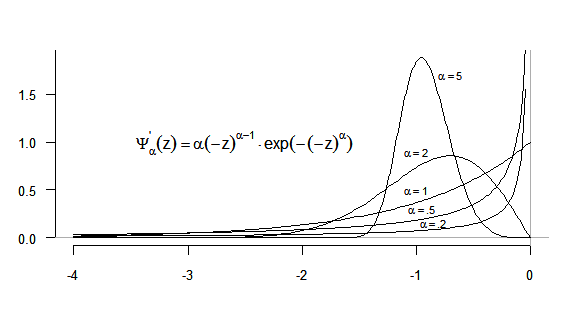
The graphs of probability densities \(\mathrm{ W’_{ \alpha } \left( z \right) = \alpha\, z^{ \alpha -1}exp \left( -z^{ \alpha } \right) \left( z \geq 0 \right) }\)for different values of \(\mathrm{ \alpha>0 }\) are given in Figure7.1.

Figure 7.1 Reduced Weibull densities (for minima).

Evidently as \(\mathrm{ W_{ \alpha } ( z ) =1- \Psi _{ \alpha } ( -z ) }\) the density \(\mathrm{ W’_{ \alpha } ( z ) }\) is the mirror image of \(\mathrm{ \Psi ’_{ \alpha } ( z ) }\).

We have

\(\mathrm{ \mu ’_{r}=M \left( Z^{r} \right) = \Gamma ( 1+{r}/{ \alpha } ) }\)

and so the mean value is \(\mathrm{ \mu = \Gamma \left( 1+{r}/{ \alpha } \right) }\), the variance \(\mathrm{ \sigma ^{2}= \Gamma \left( 1+{2}/{ \alpha } \right) - \Gamma ^{2} \left( 1+1/ \alpha \right) , }\)the corresponding values for \(\mathrm{ X}\) being obvious.

Also we have the mode \(\mathrm{ \mu ’=0 }\) if \(\mathrm{ \alpha \leq 1 }\) , \(\mathrm{ \mu ’= ( 1-1/ \alpha ) ^{1/ \alpha } }\) if \(\mathrm{ \alpha \geq 1 }\), the median \(\mathrm{ \tilde{\mu}= ( log\,2 ) ^{1/ \alpha } }\) and the \(\mathrm{ p }\) -quantil \(\mathrm{ \chi _{p}= \left(-log \left(1-p \right) \right) ^{1/ \alpha }~with~ \chi _{1-1/c}=1 }\).

Note that \(\mathrm{ \alpha \left( 1-Z \right) }\), with \(\mathrm{ Z }\) having the distribution function \(\mathrm{ W_{ \alpha } \left( z \right) }\), has mean value \(\mathrm{ \alpha ( 1- \Gamma ( 1+{1}/{ \alpha } ) ) = \gamma - ( \frac{ \pi ^{2}}{6}+ \gamma ^{2} ) /2 \alpha +O ( \alpha ^{-2} ) }\) and variance \(\mathrm{ \alpha ^{2} ( \Gamma ( 1+2/ \alpha ) ) - \Gamma ^{2} ( 1+1/ \alpha )=\frac{ \pi ^{2}}{6}+O ( \alpha ^{-1} ) }\)which suggests that \(\mathrm{ \alpha \left( 1-Z \right) }\) converges to a Gumbel distribution of maxima when \(\mathrm{ \alpha \rightarrow \infty }\) and so, for large \(\mathrm{ \alpha }\), we can use it as an approximation. The exact proof is left as an exercise.

The moment generating function of \(\mathrm{ Z }\) does not have an explicit expression but that of \(\mathrm{ log~Z }\) (which is a Gumbel random variable of minima) is

\(\mathrm{ M ( e^{ \theta\, log\,Z} ) =M ( Z^{ \theta } ) = \Gamma ( 1+ \theta / \alpha ) }\).

The computation of \(\mathrm{ \beta_1 }\) and \(\mathrm{ \beta_2 }\), also depending on \(\mathrm{ \alpha }\), is left as an exercise.

3 . Estimation and testing

Some difficulties can appear for the Weibull distribution depending on the interplay of the location \(\mathrm{ (\lambda ) }\)  and shape parameter \(\mathrm{ (\alpha ) }\) .

If \(\mathrm{ \lambda = \lambda _{0} }\)  is known, as said before, there is no problem with its reduction to the Gumbel distribution for maxima.

Let us consider first the situation when \(\mathrm{ \alpha }\) is known and \(\mathrm{\left( \lambda , \delta \right) }\)  unknown ‒ a real location-dispersion case. It is very easy to verify that if \(\mathrm{ \alpha <1, \hat{\lambda }=x’_{1}=min \left( x_{1},…,x_{n} \right) }\) and any positive statistic \(\mathrm{ \delta ^{*} \left( x_{1},…,x_{n} \right) >0 }\) are maximum likelihood estimators of \(\mathrm{\left( \lambda , \delta \right) }\) !

For \(\mathrm{ \alpha=1 }\) (exponential distribution) we have \(\mathrm{ \hat{\lambda} =x’_{1}=min \left( x_{1},…,x_{n} \right) }\)  and \(\mathrm{ \hat{\delta} =\hat{x}- \hat{\lambda} }\) , but owing to the influence of the minimum \(\mathrm{ \hat{\lambda} }\) the asymptotic behaviour of \(\mathrm{ ( \hat{\lambda} , \hat{\delta} ) }\) is not binormal, because \(\mathrm{ \hat{\lambda} }\) also has the same exponential distribution with location parameter \(\mathrm{ \lambda }\) and dispersion parameter \(\mathrm{ \delta /n }\). Note, also, that \(\mathrm{P ( \hat{\lambda} > \lambda) =1}\).

It can remarked that the minimum-variance unbiased estimators of \(\mathrm{ \lambda }\) and \(\mathrm{ \delta }\) are

\(\mathrm{ \lambda ^{*}= ( {n~x’_{1}-\bar{x} ) }/{ ( n-1 ) }= \hat{\lambda} - \hat{\delta} / ( n-1 ) }\)

and

\(\mathrm{ \delta ^{*}={n \left( \bar{x}-x’_{1} \right) }/{ \left( n-1 \right) }= \mathrm{ n~ \hat{\delta} / \left( n-1 \right)}; }\)

See Epstein and Sobel (1954) for details.

For \(\mathrm{ 1 \leq \alpha \leq 2 }\) the maximum likelihood estimators exist but the Cramér-Rao bound, using the second derivatives, does not. Other bounds, valid throughout the range of \(\mathrm{ \alpha }\), were found in Tiago de Oliveira and Littauer (1972). Are smaller than the Cramér-Rao bound in the range \(\mathrm{ \alpha > 2 }\), as shown in the paper by Tiago de Oliveira (1968).

In prediction results we will develop these bounds.

For \(\mathrm{ 1 \leq \alpha \leq 2 }\) the maximum likelihood estimator \(\mathrm{ \hat{\lambda} }\) is not asymptotically normal and whether or not it is efficient is an open question; see Woodroofe (1974). For known \(\mathrm{ \alpha < 2 }\), Tiago de Oliveira (1983) has shown that \(\mathrm{ \delta ^{* \alpha }= \sum _{i=1}^{n} \left( x_{i}-x’_{1} \right) ^{ \alpha /n} }\) has all the asymptotic properties of the maximum likelihood estimator of \(\mathrm{ \alpha }\). If \(\mathrm{ \alpha }\)  is known but \(\mathrm{ \lambda }\) and \(\mathrm{\delta}\) are unknown, the tables of Harter and Dubey (1967) can be used to test hypotheses concerning the mean value and variance.

The case where \(\mathrm{ \alpha > 2 }\) is simple and regular; see Cramér (1946). The maximum likelihood estimators of \(\mathrm{\left( \lambda , \delta \right) }\) for \(\mathrm{ \alpha=\alpha _0(> 2) }\)  known, are given by the equations

\(\mathrm{ \frac{ \sum _{1}^{n} ( x_{i}- \hat{\lambda} ) ^{ \alpha _{0}-1}}{ \sum _{1}^{n} ( x_{i}- \hat{\lambda} ) ^{ \alpha _{0}}}=\frac{ \alpha _{0}-1}{n~ \alpha _{0}} \sum _{1}^{n}\frac{1}{x_{i}- \hat{\lambda}} }\)

\(\mathrm{ \hat{\delta} = (\frac{1}{n} \sum _{1}^{n} ( x_{i}- \hat{\lambda } ) ) ^{1/ \alpha _{0}}. }\)

The random pair \(\mathrm{ ( \hat{\lambda} , \hat{\delta} ) }\)  is asymptotically normal with mean values \(\mathrm{\left( \lambda , \delta \right) }\), variances \(\mathrm{\alpha _{0}^{2}~ \delta ^{2}/n \Delta, \left( \alpha _{0}-1 \right) ^{2} ~\Gamma \left( 1-2/ \alpha _{0} \right) \delta ^{2}/n \Delta }\), covariance \(\mathrm{ - \alpha _{0} \left( \alpha _{0}-1 \right) \Gamma \left( 1-1/ \alpha _{0} \right) \delta ^{2}/n \Delta }\), and correlation coefficient \(\mathrm{\rho =- \Gamma ( 1-1/ \alpha _{0} ) /\sqrt[]{ \Gamma ( 1-2/ \alpha _{0} ) } }\), where \(\mathrm{\Delta }\) denotes

\(\mathrm{\alpha _{0}^{2} \left( \alpha _{0}-1 \right) ^{2} \left[ \Gamma \left( 1-{2}/{ \alpha _{0}} \right) - \Gamma ^{2} \left( 1-2/ \alpha _{0} \right) \right] }\).

From these results the usual tests and confidence intervals can be made. The estimator \(\hat{\lambda} + \chi _{p}\hat{ \delta } \) of the \(p\) -quantile \(\lambda + \chi _{p} \delta \) is asymptotically normal with mean value \(\lambda + \chi _{p} \delta \)  and variance

\({( \left( \alpha _{0}- \left( \alpha _{0}-1 \right) \Gamma \left( 1-{1}/{ \alpha _{0}} \right) \chi _{p} \right) ^{2}+ \left( \alpha _{0}-1 \right) ^{2} \left[ \Gamma \left( 1-{2}/{ \alpha _{0}} \right) - \Gamma ^{2} \left( 1-{1}/{ \alpha _{0}} \right) \right] \chi _{p} ) \delta ^{2}/n \Delta} \)  

\(= ( \frac{ \left( \alpha _{0} \left( \alpha _{0}-1 \right) \Gamma \left( 1-{1}/{ \alpha _{0}} \right) \chi _{p} \right) ^{2}}{ \Delta }+\frac{ \chi _{p}^{2}}{ \alpha _{0}^{2}} ) \delta ^{2}/n \)

\(= ( \frac{ \left( 1- \Gamma \left( 2-{1}/{ \alpha _{0}} \right) \chi _{p} \right) ^{2}}{ \left( \alpha _{0}-1 \right) ^{2} \left( \Gamma \left( 1-{2}/{ \alpha _{0}} \right) - \Gamma ^{2} \left( 1-{1}/{ \alpha _{0}} \right) \right) }+\frac{ \chi _{p}^{2}}{ \alpha _{0}^{2}} ) \delta ^{2}/n. \)

For prediction, the mean value of the minimum of the next \(m\)  observations is \(\lambda + \Gamma \left( 1+{1}/{ \alpha _{0}} \right) /m^{{1}/{ \alpha _{0}}}~ \delta \) . As before we use as predictor \(\hat{\lambda} + \Gamma \left( 1+{1}/{ \alpha _{0}} \right) /m^{{1}/{ \alpha _{0}}}~ \hat{\delta} \) and the mean square error of the predictor is, as we can take  \(\chi _{p}= \Gamma \left( 1+{1}/{ \alpha _{0}} \right) \) ,

\(( \Gamma \left( 1+{2}/{ \alpha _{0}} \right) - \Gamma ^{2} \left( 1+1 \left( \alpha _{0} \right) \right) \delta ^{2}+ \)

\(( \frac{1- \Gamma \left( 2-{1}/{ \alpha _{0}} \right)~ \Gamma \left( 1+1 \left( \alpha _{0} \right) \right) ^{2}}{ \left( \alpha _{0}-1 \right) ^{2}~ \left( \Gamma \left( 1-{2}/{ \alpha _{0}} \right) - \Gamma ^{2} \left( 1-{1}/{ \alpha _{0}} \right) \right) }+\frac{ \Gamma ^{2} \left( 1+{1}/{ \alpha _{0}} \right) }{ \alpha _{0}^{2}} ) \delta ^{2}/n \) .

Let us now consider the 3-parameter Weibull distribution. The state of affairs in this case is very awkward, chiefly because we have to estimate \(\mathrm{ \alpha }\) with a global behaviour changing according to its real value; see Dubey (1967) and (1967’) and Mann (1968) to get the first feelings of the difficulties of the problem, chiefly connected with the non-existence of maximum likelihood estimators for all values of \(\mathrm{ \alpha }\). Cohen and Whitten (1982) advise that one should attempt to obtain maximum likelihood estimators for the three-parameter Weibull distribution unless there is reason to expect \(\mathrm{ \alpha >2.2}\).

With all these restrictions, let us write the maximum likelihood equations. From the likelihood of the sample \(\mathrm{ \left( x_{1},…,x_{n} \right) }\)     

\(\mathrm{ L \left( \lambda , \delta , \alpha \vert x_{i} \right) =0 }\)                      if          \(\mathrm{ min \left( x_{1},…,x_{n} \right) \leq \lambda }\)

\(\mathrm{ L \left( \lambda , \delta , \alpha \vert x_{i} \right) =\frac{ \alpha ^{n}}{ \delta ^{ \alpha n}}\begin{array}{c} \mathrm{n} \\ \mathrm{\pi} \\ \mathrm{1} \end{array}~ \left( x_{i}- \lambda \right) ^{ \alpha -1}exp \{ - \sum _{1}^{n} ( \frac{x_{i}- \lambda }{ \delta } ) ^{ \alpha } \} ~if\,min \left( x_{1},…,x_{n} \right) > \lambda }\)

we get

\(\mathrm{ \hat{\delta} \hat{\alpha }=\frac{1}{n} \sum _{1}^{n} ( x_{i}- \hat{\lambda} ) ^{\hat{ \alpha} } }\)

\(\mathrm{ \frac{ \hat{\alpha} -1}{ \hat{\alpha} } \sum _{1}^{n}\frac{1}{x_{i}- \hat{\lambda} }=\frac{n \sum _{1}^{n}( x_{i}- \hat{\lambda} ) ^{ \hat{\alpha} -1}}{ \sum _{1}^{n} ( x_{i}- \hat{\lambda} ) ^{ \hat{\alpha} }} }\)

\(\mathrm{ \frac{1}{\hat{ \alpha} }+\frac{1}{n} \sum _{1}^{n}log ( x_{i}- \hat{\lambda} ) = \sum _{1}^{n} ( x_{i}- \hat{\lambda} ) ^{ \hat{ \alpha} }~log ( x_{i}- \hat{\lambda} ) / \sum _{1}^{n} ( x_{i}- \hat{\lambda} ) ^{\hat{ \alpha} }. }\)

For this system we have to solve for \(\mathrm{ ( \hat{\lambda} , \hat{\alpha} ) }\), as a first step, the last two equations and then compute \(\mathrm{\hat{ \delta} }\).If \(\mathrm{ \alpha > 2 }\) the system is asymptotically trinormal and the previous techniques applied to the Fréchet distribution can be used. Those equations can be compared, and are similar, to those for the Fréchet distribution of maxima, as could be expected. Also it can be shown that:

The random triple \((\hat{\lambda} , \hat{\delta} , \hat{\alpha } )\)  is asymptotically trinormal with mean values \((\hat{\lambda} , \hat{\delta} , \hat{\alpha } )\) if \(\alpha>2\) and variance-covariance matrix analogous to the one for Fréchet distribution.

The real important situations are considered below, particularly in the subsection “The maximum likelihood estimator when \(\mathrm{\alpha_0>2}\) ".

The usual techniques of confidence interval estimation and hypothesis testing can be applied as before. Prediction will be discussed in the next section.

Lemon (1975) modified the likelihood equations so that one need iteratively solve only two equations for estimates of \(\mathrm{ \lambda }\) and \(\mathrm{ \alpha }\), which together then specify an estimate of \(\mathrm{\delta}\) . Cohen and Whitten (1982) suggest other modifications to the maximum likelihood methods which involve simplification of one of the equations.

For estimation of the three Weibull parameters, the method of moments seems to work well, in general, as estimators can always be obtained. The tables of Dubey (1967) applying to the two-parameter distribution, and the Monte Carlo results of Cohen and Whitten (1982) applying to the three-parameter distribution, indicate that the moment estimators are very efficient for \(\mathrm{ \alpha =4.7}\) and become progressively less efficient as \(\mathrm{ \alpha }\) converges towards 2 or towards \(\mathrm{ + \infty. }\) Cohen and Whitten (1982) provide a table which facilitates estimation of \(\mathrm{ \alpha }\) from the distribution skewness coefficient \(\mathrm{\beta_1}\).These authors also give several modifications to the moment equations which simplify estimation of all three parameters.

Another iterative procedure for estimating \(\mathrm{ \lambda }\) is one by Mann and Fertig (1973). If \(\mathrm{ \alpha }\) is not too large, this method also provides a lower confidence bound for \(\mathrm{ \lambda }\). Also we can use the proposed statistic to test \(\mathrm{ \lambda =0}\)  vs. \(\mathrm{ \lambda >0}\), which is very important in fatigue failure research. The basic statistic for this test is a ratio of selected sums of differences of successive ordered logarithms of sample observations, each difference being divided by its expected value. To obtain a point estimate of \(\mathrm{ \lambda }\) (which is median unbiased) or a lower confidence bound, the initial guess of \(\mathrm{ \lambda }\) must be subtracted from each observation and iterated until the modified statistic is numerically equal to a percentile of the statistics distribution. The method has two advantages: the test statistic, under \(\mathrm{ \alpha =0}\) , has a Beta distribution, and it is appropriate for use with censored data. The later advantage can also be claimed for a similar statistic by Weissman (1978) and for certain linear estimators of \(\mathrm{-log\,\delta}\) and \(\mathrm{ \alpha ^{-1}}\) that can be applied to the ordered logarithms of the observed data after an estimate of \(\mathrm{ \lambda }\) is subtracted from each of the original values.

Wyckoff, Bain and Engelhardt (1980) suggest the use of a simplified linear estimator of \(\mathrm{ \alpha ^{-1}}\), after having substituted \(\mathrm{ \lambda }\) by a simple estimator, as an approximation of the best linear unbiased estimator. This seems to yield appropriate and quite efficient estimates for \(\mathrm{ \alpha ^{-1}}\), and ultimately for \(\mathrm{log\,\delta}\), if \({\mathrm​​​​\alpha\leq3.0}\)  when there is no censoring (or if \(\mathrm{ \alpha }\) is somewhat less than 3.0 when there is censoring). For larger values of \(\mathrm{ \alpha }\), estimates of \(\mathrm{ \alpha ^{-1}}\) obtained by this method have a substantial negative bias unless sample size is extremely large.

Besides the linear estimators of \(\mathrm{log\,\delta}\)  and  \(\mathrm{ \alpha ^{-1}}\), there are other simple estimators of the Weibull parameters that are appropriate for use under certain conditions. For \({​​​​\alpha\leq1}\), a special case suggested by Zanakis (1979) of the estimator of \(\mathrm{ \lambda }\)  previously proposed by Dubey (1966), namely, \(\mathrm{​​​​ \lambda ’= ( x_{1}^{’}~x_{n}^{’}-x_{2}^{’2} ) / ( x_{1}^{’}+x_{n}^{’}-2~x_{2}^{’} ) }\), has relatively small bias and mean-square error. For \(\mathrm{​​​​\alpha>1}\), a statistic investigated by Kappenam (1981) has smaller bias and mean-square error than the last one for estimating \(\mathrm{ \lambda }\), but is also considerably more difficult to compute, involving a weighted average of all the order statistics.

Zanakis and Mann (1982) compared two simple estimators of \(\mathrm{ \alpha }\)  based on a few order statistics:

\(\mathrm{​​​​ \alpha _{1}^{*}=log [ ( {x_{k}^{’}-x_{j}^{’} ) }/{ ( x_{j}^{’}-x_{i}^{’}} ) ] /3.643 }\)

and   \(\mathrm{​​​​ \alpha _{2}^{*}=log [ ( x_{m}^{’}- \lambda ’ ) / ( x_{h}^{’}- \lambda ’) ] /2.989 }\)

with   \(\mathrm{​​​​ 1 \leq i<j<k \leq n,~1 \leq h<m \leq n }\) defined appropriately and \(\mathrm{ \lambda '}\)  given above.

They found both estimators to be good for small values of \(\mathrm{ \alpha }\), but having more negative bias than estimators based on the procedures prescribed by Wyckoff, Bain and Engelhardt (1980). The simple estimators are useful for first guesses in maximum-likelihood estimation and in other situations in which quick results are necessary.

4 . Point prediction

As before, the mean-square point predictor of the minimum of the next \(\mathrm{ m }\) observations is evidently the estimator of the mean value of \(\mathrm{ W=min ( Y_{1},...,Y_{n} ) . }\) The distribution of \(\mathrm{ W}\) is, as seen before, \(\mathrm{ W_{ \alpha } ( \frac{x- \lambda }{ \delta ~m^{-1/ \alpha }} ) }\) if the distributions of \(\mathrm{ Y_j}\), as well as those of \(\mathrm{ x_j}\), are \(\mathrm{W_{ \alpha } ( \left( x- \lambda \right) / \delta )}\). The mean value of \(\mathrm{ W}\)  is

\(\mathrm{ M ( W ) = \lambda +m^{-1/ \alpha } \Gamma \left( 1+1/ \alpha \right) \delta }\) ,

and thus a point predictor of \(\mathrm{ W}\) can be obtained substituting \(\mathrm{ ( \lambda, \delta , \alpha ) }\) by their estimators. But difficulties exist when \(\mathrm{ \lambda }\) is not known and \(\mathrm{ \alpha}\) may be \(\mathrm{ \leq2}\). If \(\mathrm{ \alpha = \alpha _{0} }\) is known and \(\mathrm{ \alpha _{0}>2 }\) (practically speaking \(\mathrm{ \alpha _{0}>2.1 }\)), there are no difficulties with the maximum likelihood estimation; likewise if \(\mathrm{ ( \lambda, \delta , \alpha ) }\) are all unknown but it is known that \(\mathrm{ \alpha >2 }\). The general theory used before for the Fréchet distribution can also be applied here.

If \(\mathrm{ \lambda = \lambda _{0} }\) is known then \(\mathrm{ -log \left( x= \lambda _{0} \right) }\) has a Gumbel distribution with location and dispersion parameters \(\mathrm{-log\,\delta}\) and \(\mathrm{ \alpha^{-1} }\) and estimation can be dealt with by the methods of Chapter 5.

The theory of best quasi-linear prediction when \(\mathrm{ \alpha = \alpha _{0} }\) leads to an unmanageable formula for the predictor, following Tiago de Oliveira (1966) as we will recall briefly.

Later we will make considerable use of Tiago de Oliveira and Littauer (1976) .

The likelihood of the observed sample is                                         

\(\mathrm{ \bar{L}_{ \alpha _{0}} ( \lambda , \delta \vert x_{i} ) =0 }\)              if          \(\mathrm{ min ( x_{i} ) > \lambda }\)

\(\mathrm{\bar{L}_{ \alpha _{0}} ( \lambda , \delta \vert x_{i} ) =\mathrm{ \begin{matrix} n \\ \pi \\ 1 \end{matrix}} \{ \frac{1}{ \delta }W’_{ \alpha _{0}} ( \frac{x_{i}- \lambda }{ \delta } ) \} }\)         if    \(\mathrm{ min ( x_{i} ) > \lambda }\)

and the likelihood of the sample and the future minimum \(\mathrm{ W}\) from \(\mathrm{ m }\)  observations is

\(\mathrm{ L_{ \alpha _{0}} ( \lambda , \delta \vert x_{i},w ) =\bar{L}_{ \alpha _{0}}( \lambda , \delta \vert x_{i},…,x_{n} ) \frac{1}{ \delta m^{-1/ \alpha _{0}}}W’_{ \alpha _{0}} ( \frac{w-\lambda}{ \delta m^{-1/ \alpha _{0}}} ) }\)

where \(\mathrm{ W_{ \alpha } \left( z \right) }\)  was defined above.

According to the paper previously cited, the mean-square predictor has the expression

\(\mathrm{p_{m} \left( x_{i} \right) =\frac{ \int _{0}^{+ \infty}d \xi ~ \xi ^{n-1} \int _{- \infty}^{+ \infty}d \eta ~\bar{L }\left( \eta + \xi ~x_{1},…,~ \eta + \xi ~x_{n} \right) \left[ \mu _{m} \left( \eta + \xi ~x_{1},…, \eta + \xi x_{n} \right) - \eta \right] }{ \int _{0}^{+ \infty}d \xi ~ \xi ^{n} \int _{- \infty}^{+ \infty}d \eta ~\bar{L} \left( \eta + \xi ~x_{1},…,~ \eta + \xi ~x_{n} \right) } }\)  

where \(\mathrm{ \bar{L }( z_{1},…,~z_{n} ;v)}\) denotes the likelihood of the first sample and the minimum of the second sample, \(\mathrm{ \bar{L }( x_{1},…,x_{n} ) = \int _{- \infty}^{+ \infty}d~v~L ( x_{1},…,x_{n};v ) }\) is the marginal likelihood of the sample, and

\(\mathrm{\mu _{m} ( x_{i} ) = \int _{- \infty}^{+ \infty}d~v~v~L ( x_{1},…,x_{n};v ) /\bar{L} ( x_{1},…,x_{n} ) }\)

is the conditional mean. As it is irrelevant, from the expression of \(\mathrm{p_{m} ( x_{i} ) }\), we can always suppose \(\mathrm{ \lambda =0 }\)  and \(\mathrm{ \delta =1 }\). This predictor was shown in that paper to be quasi-linear, i.e., \(\mathrm{p_{m} ( \lambda + \delta ~x_{i} ) = \lambda + \delta ~p_{m} ( x_{i} ) }\), for every \(\mathrm{ \lambda }\) and \(\mathrm{ \delta(>0) }\) .

Note that, in our case, we have

\(\mathrm{\mu _{m} \left( x_{i} \right) = \mu _{ \alpha _{0,m}}= \int _{- \infty}^{+ \infty}~d~v~m^{1/ \alpha _{0}}~v~W_{ \alpha }^{’} \left( m^{1/ \alpha _{0}}~v \right) ={ \Gamma \left( 1+{1}/{ \alpha _{0}} \right) }/{m^{{1}/{ \alpha _{0}}}}= \mu _{ \alpha _{0}},1/m^{1/ \alpha _{0}}0. }\)

and    \(\mathrm{\bar{L} ( x_{i} ) =L_{ \alpha _{0}} ( x_{i} ) }\).

As \(\mathrm{ W’_{ \alpha _{0}}( z ) =0~if~z \leq 0 }\), the integration takes place in the region \(\mathrm{ \alpha + \beta ~x_{i} \geq 0 }\), that is, \({ \alpha \geq - {\beta} ~l \mathrm{( x_{i} ) }}\) where \(l\mathrm{ \left( x_{i} \right) =min( x_{1},…,x_{n} ) }\).

The predictor can be written as

\(\mathrm{ p_{ \alpha _{0}},m ( x_{i} ) =\frac{ \int _{0}^{+ \infty}d \xi ~ \xi ^{n-1} \int _{\mathit{l} ( x_{i} ) }^{+ \infty}d \eta ( \mu _{ \alpha _{0,}m^{- \eta }} ) \begin{array}{c} \mathrm{n} \\ \mathrm{\pi} \\ \mathrm{i=1} \end{array}W’_{ \alpha _{0}} ( \eta + \xi ~x_{i} ) }{ \int _{0}^{+ \infty}d \xi ~ \xi ^{n}~ \int _{\mathit{l} ( x_{i} ) }^{+ \infty}d \eta \begin{array}{c} \mathrm{n} \\ \mathrm{\pi} \\ \mathrm{i=1} \end{array}W’_{ \alpha _{0}} \left( \eta + \xi ~x_{i} \right) }. }\)

Putting \(\mathrm{ \zeta = \xi + \eta }\,l\mathrm{ ( x_{i} ) }\) we get

\(\mathrm{ p_{ \alpha _{0},m} ( x_{i} ) =\mathit{l} \left( x_{i} \right) +\frac{ \int _{0}^{+ \infty}d \xi ~ \xi ^{n-1} \int _{0}^{+ \infty}d~ \zeta ( \mu _{ \alpha _{0,}m^{- \zeta }} )\begin{array}{c} \mathrm{n} \\ \mathrm{\pi} \\ \mathrm{i=1} \end{array} W’_{ \alpha _{0}} \left( \zeta + \xi \left( x_{i}-\mathit{l} \left( x_{i} \right) \right) \right) }{ \int _{0}^{+ \infty}d \xi ~ \xi ^{n} \int _{0}^{+ \infty}d~ \zeta\begin{array}{c} \mathrm{n} \\ \mathrm{\pi} \\ \mathrm{i=1} \end{array} W’_{ \alpha _{}} \left( \zeta + \xi ~ \left( x_{i}-\mathit{l}\left( x_{i} \right) \right) \right) }. }\)  

It is evident that computation facilities will not be useful at all, as the expression above implies the computation of the predictor \(\mathrm{ p_{ \alpha _{o},m} ( x_{i} ) }\) for any \(\mathrm{ n }\) (sample size) and for any (practically) observable sample mean, except for special cases. For example, in the case of the exponential distribution \(\mathrm{ ( \alpha _{0}=1 ) }\), we have

\(\mathrm{ W’_{1} ( z ) =0 }\)                if             \(\mathrm{ z \leq 0 }\)

\(\mathrm{ =e^{-z}}\)                        if            \(\mathrm{ z \geq 0 }\),

\(\mathrm{ \mu _{1,m}=1/m }\), and thus we obtain

\(\mathrm{ P1,m ( x_{i} ) =\mathit{l} ( x_{i} ) + ( \frac{1}{m}-\frac{1}{n} ) [ x-\mathit{l} ( x_{i} ) ] }\) .

5 . Lower bounds for the mean-square error

As the maximum likelihood estimators are not regular or do not exist if \(\mathrm{ \alpha \leq 2 }\), it is natural to search for a quasi-linear predictor and thus to try to obtain a lower bound for the mean-square error of any quasi-linear statistic \(\mathrm{ f ( x_{i} ) }\) for \(\mathrm{ \lambda + \mu _{ \alpha _{o},m}~ \delta }\) .

The mean-square error of a quasi-linear statistic \(\mathrm{ f ( x_{i} ) }\) is

\(\mathrm{ M \left( f ( x_{i} )-W \right) ^{2}= \delta ^{2}\,M ( f ( z_{i} ) -v ) ^{2} }\)

where \(\mathrm{ x_{i}= \lambda + \delta ~z_{i} }\) and \(\mathrm{ w= \lambda + \delta ~v }\) (i.e., \(\mathrm{ z_i }\) and \(\mathrm{ v }\) are the reduced values of the observations). From now on we will deal, thus, with reduced observations \(\mathrm{ (\lambda =0, \delta =1)}\) because we are going to evaluate efficiencies and the factor \(\mathrm{ \delta^2 }\) cancels out.

The values of \(\mathrm{ M ( f ( z_{i} ) -v ) ^{2} }\) can be split simply by putting \(\mathrm{ f ( z_{i} )-v= ( f ( z_{i} ) - \mu _{ \alpha _{0},m} ) - ( v- \mu _{ \alpha _{0},m} ) }\)and so, by independence between the first and second sample, we have

\(\mathrm{ M ( f ( z_{i} ) -v ) ^{2}=M ( f ( z_{i} ) - \mu _{ \alpha _{0},m} ) ^{2}+M ( v- \mu _{ \alpha _{0},m} ) ^{2} }\)

\(\mathrm{ =D_{n,m}^{2} \left( f \right) + \sigma _{m}^{2} \left( \alpha _{0} \right) =mean-square~error~of~f ( z_{i} ) ~about~ \mu _{ \alpha _{0},m}+variance~of~v. }\)  

Thus we will study \(\mathrm{ D_{n,m}^{2} ( f ) }\) . It was shown in Tiago de Oliveira (1968), using the Schwarz inequality conveniently, that, in the general case, if we denote by \(\mathrm{ \varphi ( \lambda , \delta ) ( - \infty< \lambda < \infty,0< \delta < \infty ) }\)  

\(\mathrm{ \int _{- \infty}^{+ \infty}… \int _{- \infty}^{+ \infty} \mu _{m} \left( \lambda + \delta ~z_{1},…, \lambda + \delta ~z_{n} \right) \bar{L} \left( z_{1},~…,z_{n} \right) dz_{1}…dz_{n} }\)

and by \(\mathrm{ w_{n}( \lambda , \delta ) }\)

\(\mathrm{ \int _{- \infty}^{+ \infty}… \int _{- \infty}^{+ \infty}\frac{\bar{L}^{2} \left( z_{1},…,z_{n} \right) }{ \delta ^{n}\bar{L} \left( \lambda + \delta ~z_{1},…, \lambda + \delta ~z_{n} \right) }~dz_{1}…dz_{n} }\) .

then

\(\mathrm{ B^{2}=sup_{ \lambda , \delta }\frac{ \left( \lambda - \varphi \left( \lambda , \delta \right) + \varphi \left( 0,1 \right) \delta \right) ^{2}}{w_{n} \left( \lambda , \delta \right) -2~ \delta + \delta ^{2}}~~~ }\)

is a lower bound for the mean-square error \(\mathrm{ D_{n,m}^{2} ( f ) =M ( f ( z_{i} ) - \mu _{m} ( z_{i} ) ) ^{2} }\) of a quasi-linear statistic \(\mathrm{ f ( z_{i}) }\) \(\mathrm{ ( when~ \lambda =0, \delta =1 ) }\). In the expression of \(\mathrm{ w_{n}( \lambda , \delta ) }\) in the integrals the indeterminate ratio  \(\mathrm{ \frac{0}{0} }\) is taken to be equal to zero.

\(\mathrm{ B^2 }\) is indeterminate for \(\mathrm{ \lambda =0, \delta =1}\). In our case, owing to independence, we have

\(\mathrm{ \varphi ( \lambda , \delta ) = \mu _{ \alpha _{0},m} }\)    and     \(\mathrm{ w_{n} ( \lambda , \delta ) =w_{ \alpha _{0}}^{n} ( \lambda , \delta ) }\)

where

\(\mathrm{ w_{ \alpha _{0}} ( \lambda , \delta ) = \int _{- \infty}^{+ \infty}\frac{W’_{ \alpha _{0}} ( z ) ^{2}}{ \delta ~W’_{ \alpha _{0}} ( \lambda + \delta z ) }~dz }\)

and thus we have

\(\mathrm{ B^{2}=sup_{ \lambda , \delta }\frac{ ( \lambda + \delta ~ \mu _{ \alpha _{0},m}- \mu _{ \alpha _{0},m} ) ^{2}}{w_{ \alpha _{0}}^{n} ( \lambda , \delta ) -2~ \delta + \delta ^{2}}. }\)

As \(\mathrm{ B^2 }\) is almost impossible to obtain, we will put \(\mathrm{ \lambda=0 }\)  above and compute

\(\mathrm{ \bar{B}^{2}=sup_{ \lambda , \delta }\frac{ \mu _{ \alpha _{0},m}^{2} \left( 1- \delta \right) ^{2}}{w_{ \alpha _{0}}^{n} \left( 0, \delta \right) -2~ \delta + \delta ^{2}} \leq B^{2} }\).

and as

\(\mathrm{ w_{ \alpha _{0}} ( 0, \delta ) =1/ [ \delta ^{ \alpha _{0}} ( 2- \delta ^{ \alpha _{0}} ) ] }\)             for     \(\mathrm{ 0< \delta ^{ \alpha _{0}}<2, }\)

we get the (smaller) lower bound

\(\mathrm{\bar{B}^{2}=\frac{ \mu _{ \alpha _{0},m}^{2}}{1+n~ \alpha _{0}^{2}} \sim \frac{ \mu _{ \alpha _{0},m}^{2}}{n~ \alpha _{0}^{2}}=\frac{ \mu _{ \alpha _{0},1}^{2}}{n~ \alpha _{0}^{2}~m^{2/ \alpha _{0}}} }\)

and an (under) evaluation of efficiency is

\(\mathrm{lim\frac{\bar{B}^{2}}{D_{n,m}^{2} \left( f \right) }=\frac{ \mu _{ \alpha _{0},1}^{2}}{ \alpha _{0}^{2}~m^{{2}/{ \alpha _{0}}}lim~n~D_{n,m}^{2} \left( f \right) } }\).

For \(\mathrm{\alpha _{0}=1,\bar{B}^{2} \sim D_{n,m}^{2} ( f ) }\) when \(\mathrm{f ( x_{i} ) =\mathit{l} ( x_{i} ) + ( \frac{1}{m}-\frac{1}{n} ) [ \bar{x}-\mathit{l}~ ( x_{i} ) ] }\) is the best predictor for the exponential distribution, already given.

In case of regularity, as happens for \(\mathrm{\alpha _{0}>2 }\), we can obtain bounds analogous to the Cramer-Rao bounds for estimation. In the last paper referred to it was shown, for the case of independence with the density \(\mathrm{g ( z ) }\) for the (reduced) \(\mathrm{ z_{i} }\) and the mean \(\mathrm{ \mu_m }\) for \(\mathrm{ v }\) , to have the expression

\(\mathrm{ B’^{2} \sim \frac{S_{0} \mu _{m}^{2}-2~S_{1}~ \mu _{m}+S_{2}-1}{n ( S_{0}~S_{2}-S_{1}^{2}-S_{0} ) } }\)

with

\(\mathrm{ S_{0}= \int _{- \infty}^{+ \infty}x^{p}~\frac{g’ ( x ) ^{2}}{g ( x ) }~d~x }\)

Putting \(\mathrm{ g ( z ) =W’_{ \alpha _{0}} ( z ) }\) and \(\mathrm{ \mu _{m}= \mu _{ \alpha _{0},m} }\) we get, as

\(\mathrm{ S_{p}=[( \alpha _{0}-1 ) ^{2}+p ( \alpha _{0}+p-2 ) ] \Gamma ( 1+\frac{p-2}{ \alpha _{0}} ) }\),

\(\mathrm{ B’^{2} \sim \frac{ \alpha _{0}^{2}-2~ \alpha _{0} \left( \alpha _{0}-1 \right) \Gamma \left( 1-{1}/{ \alpha _{0}} \right) \mu _{ \alpha _{0},m}+ \left( \alpha _{0}-1 \right) ^{2}~ \Gamma \left( 1-{2}/{ \alpha _{0}} \right) ~ \mu _{ \alpha _{0},m}^{2}}{n~ \alpha _{0}^{2} \left( \alpha _{0}-1 \right) ^{2}~ \left[ \Gamma \left( 1-{2}/{ \alpha _{0}} \right) - \Gamma ^{2} \left( 1-{1}/{ \alpha _{0}} \right) \right] } }\)

Asymptotically we have \(\mathrm{ \bar{B}^{2} \leq B’^{2} }\) and so the (under-) evaluation of  the efficiency is to be taken as

\(\mathrm{ B’^{2}/D_{n,m}^{2} ( f ) }\)

In fact, as the maximum likelihood estimators are the best when regular \(\mathrm{ ( \alpha _{0}>2 ) }\), we are going to obtain a set of simple predictors, chiefly for  \(\mathrm{ \alpha _{0} \leq 2 }\), such that they have reasonably good efficiency for some interval in \(\mathrm{ [ 0,2 ]}\).

6 . Some predictors for the shape parameter α_o≤2

It is desirable to explore different predictors for different ranges of \(\mathrm{ \alpha _{0}}\)  because of computational difficulties. Let us begin by examining the region \(\mathrm{ \alpha _{0} \leq 2}\), with a suggestion from the result for the exponential \(\mathrm{ (\alpha _{o}=1 )}\) . 

The simple predictor for the exponential distribution suggests the use of the statistic

\(\mathrm{\mathit{l} ( x_{i} ) +a ( \alpha _{0} ) ( \bar{x}-\mathit{l} ( x_{i} ) ) }\)

as predictor, where \(\mathrm{ a(\alpha_0) }\) is to be determined so as to minimize the mean-square error, which for reduced values is

\(\mathrm{ D_{n,m}^{2}=M ( \mathit{l} ( x_{i} ) +a ( \alpha _{0} ) ( \bar{x}-\mathit{l} ( x_{i} ) ) - \mu _{ \alpha _{0},m} ) ^{2} }\).

This predictor is suggested also by the fact that the lower limit \(\mathrm{ \lambda }\) has \(\mathrm{ \mathit{l}(x_i) }\) as a sufficient estimator (but an over-estimator).

The sample average is a quasi-linear statistic converging to \(\mathrm{ \mu _{ \alpha _{0},1}= \lambda + \delta\, \Gamma ( 1+{1}/{ \alpha _{0}} ) }\) , with variance \(\mathrm{ \delta ^{2}~b ( \alpha _{0} ) /n }\) with 

\(\mathrm{ b ( \alpha _{0} ) = [ \Gamma ( 1+{2}/{ \alpha _{0}} ) - \Gamma ^{2} ( 1+{1}/{ \alpha _{0}} ) ] }\);

\(\mathrm{ \mathit{l}(x_i) }\) has the mean value \(\mathrm{ \mu _{ \alpha _{0},n}= \lambda + \delta ~ \Gamma ( 1+{1}/{ \alpha _{0}} ) /n^{1/ \alpha _{0}} }\), its variance being \(\mathrm{ \delta ^{2}~b \left( \alpha _{0} \right) /n^{2/ \alpha _{0}} }\) the correlation coefficient \(\mathrm{ \rho _{ \alpha _{0},n}= \rho ( \bar{x},\mathit{l} ( x_{i} ) ) }\) converges to zero; see Tiago de Oliveira (1962) and Rosengard (1966).

Thus, the mean-square error \(\mathrm{ D_{n,m}^{2} }\) for reduced observations as a function of \(\mathrm{ a }\), can be written as \(\mathrm{ M \left[ \mathit{l} \left( x_{i} \right) +a \left( \bar{x}-\mathit{l} \left( x_{i} \right) \right) - \mu _{ \alpha _{0},m} \right] ^{2}=M \left[ \mathit{l} \left( x_{i} \right) - \mu _{ \alpha _{0},m} \right] ^{2}+2~M \left[ \left( \mathit{l} \left( x_{i} \right) - \mu _{ \alpha _{0},m} \right) \left( \bar{x}-\mathit{l} \left( x_{i} \right) \right) \right] a+M \left[ \bar{x}-\mathit{l} \left( x_{i} \right) \right] ^{2}a^{2}. }\) Using the decomposition \(\mathrm{\mathit{l} \left( x_{i} \right) - \mu _{ \alpha _{0},m}=\mathit{l} \left( x_{i} \right) - \mu _{ \alpha _{0},n}+ \mu _{ \alpha _{0},n}- \mu _{ \alpha _{0},m} }\) and \(\mathrm{\bar{x}-\mathit{l} \left( x_{i} \right) =\bar{x}- \mu _{ \alpha _{0},1}+ \mu _{ \alpha _{0},1}- \mu _{ \alpha _{0},n}+ \mu _{ \alpha _{0},n}-\mathit{l} \left( x_{i} \right) }\), we have

\(\mathrm{ M [ (\mathit{l} \left( x_{i} \right) - \mu _{ \alpha _{0},m} ) ^{2} ] =\frac{b ( \alpha _{0} ) }{n^{{2}/{ \alpha _{0}}}}+ ( \mu _{ \alpha _{0},n}- \mu _{ \alpha _{0},m} ) ^{2}, }\)

\(\mathrm{ M \left[ \left( \mathit{l} \left( x_{i} \right) - \mu _{ \alpha _{0},m} \right) \left( \bar{x}-\mathit{l} \left( x_{i} \right) \right) \right] = \rho _{ \alpha _{0},n} \frac{b \left( \alpha _{0} \right) }{n^{{2}/{ \alpha _{0}}+{1}/{2}}}-\frac{b \left( \alpha _{0} \right) }{n^{{2}/{ \alpha _{0}}}}+ }\)

\(\mathrm{( \mu _{ \alpha _{0},n}- \mu _{ \alpha _{0},m} ) ( \mu _{ \alpha _{0},1}- \mu _{ \alpha _{0},n} ) , }\)

\(\mathrm{ M \left[ (\bar{x}-\mathit{l} \left( x_{i} \right) \right) ^{2} ] =\frac{b \left( \alpha _{0} \right) }{n}+ \left( \mu _{ \alpha _{0},1}- \mu _{ \alpha _{0},n} \right) ^{2}+\frac{b \left( \alpha _{0} \right) }{n^{2/ \alpha _{0}}}-2 \rho _{ \alpha _{0},n}\frac{b \left( \alpha _{0} \right) }{n^{1/ \alpha _{0}+1/2}}. }\)  

The minimum of the quadratic is attained at some value whose limit is

\(\mathrm{ -a \left( \alpha _{0} \right) ={ \mu _{ \alpha _{0},m}}/{ \mu _{ \alpha _{0},1}}=m^{-1/ \alpha _{0}} }\),

thus the predictor is \(\mathrm{ \mathit{l} ( x_{i} ) +m^{-1/ \alpha _{0}} ( \bar{x}-\mathit{l} ( x_{i} ) ) }\). The asymptotic values of the mean-square error are then:

\(\mathrm{ D_{n,m}^{2}=\frac{ \mu _{ \alpha _{0},m}^{2}~b \left( \alpha _{0} \right) }{ \mu _{ \alpha _{0},1}^{2}~n}=\frac{b \left( \alpha _{0} \right) }{n~m^{2/ \alpha _{0}}} }\)                if    \(\mathrm{ \alpha _{0}<2 }\) ,

\(\mathrm{ D_{n,m}^{2} \sim \frac{m-2~\sqrt[]{m}+2- \pi /4}{m~n}}\)                        if    \(\mathrm{ \alpha _{o}=2, }\)

\(\mathrm{ D_{n,m}^{2} \sim \frac{ \Gamma \left( 1+2/ \alpha _{0} \right) \left( 1-m^{-1/ \alpha _{0}} \right) ^{2}}{n^{2/ \alpha _{0}}}}\)                 if   \(\mathrm{ \alpha _{0}>2. }\)

Consequently, the asymptotic efficiency is, since \(\mathrm{ \bar{B}^{2} \sim \frac{ \mu _{ \alpha _{0},m}^{2}}{n~ \alpha _{0}^{2}}, }\)

\(\mathrm{ eff \left( \alpha _{0} \right) =\frac{ \Gamma ^{2} \left( 1+{1}/{ \alpha _{0}} \right) }{ \alpha _{0}^{2}~b \left( \alpha _{0} \right) } }\)                         if   \(\mathrm{ \alpha _{0}<2 }\)

\(\mathrm{ eff~ \left( \alpha _{o} \right) ~=\frac{ \pi }{16 \left( m~-~2~\sqrt[]{m}~+~2-~ \pi /4 \right) } }\)        if   \(\mathrm{ \alpha _{o}=2, }\)

\(\mathrm{ eff~ \left( \alpha _{o} \right) =0 }\)                                     if   \(\mathrm{ \alpha _{0}>2. }\)

Zero efficiency for \(\mathrm{ \alpha _{0}>2 }\) results from the slow convergence of \(\mathrm{ \mathit{l}(x_i) }\) to the parameter \(\mathrm{ \lambda }\), an effect that in this region overcomes the more rapid convergence of the average \(\mathrm{ \bar{x} }\). The efficiency for \(\mathrm{ \alpha _{0}>2 }\) is independent of \(\mathrm{ m }\). A short table of the efficiency for the above predictor is, for \(\mathrm{ m=1 }\) .

\(\mathrm{\begin{matrix} {\alpha_0} & 1/3&1/2&1&2^-\\ {\mathrm{eff(\alpha_0)}} & 0.5&0.8&1&0.91\,. \end{matrix}}\)

The predictor for \(\mathrm{ 1/2< \alpha _{0}<2 }\) is thus reasonably efficient. Outside this range for the shape parameter, another predictor must be found.

Consider now the usage of a sample quantile \(\mathrm{Q(x_i)}\) and the minimum value \(\mathrm{\mathit{l}(x_i)}\). It is apparent (by the argument given above), that, since the variance of a quantile is of order \(\mathrm{ 1/n }\), a linear combination

\(\mathrm{ \mathit{l} ( x_{i} ) +a ( \alpha _{0} ) ( Q ( x_{i} ) -\mathit{l} ( x_{i} ) ) }\)

may be efficient only in the region \(\mathrm{\alpha _{0} \leq 2 }\) ; it will be useful in the region \(\mathrm{\alpha _{0}<1/2 }\).  For known \(\mathrm{\alpha = \alpha _{0} }\), let us denote by \(\mathrm{\upsilon }\) the quantile of probability \(\mathrm{\omega =W_{ \alpha _{0}} \left( \upsilon \right) }\). It is well known (Cramér, 1946) that the sample quantile \(\mathrm{Q(x_i)}\) for probability \(\mathrm{\omega}\), with reduced observations, is asymptotically normal with expected value \(\mathrm{\upsilon }\) and asymptotic variance of the order of \(\mathrm{ \omega \left( 1- \omega \right) /n{W^{’2}_{ \alpha _{0}}} \left( \upsilon \right) }\) .   As

\(\mathrm{W_{ \alpha _{0}} \left( z \right) =1-e^{-z^{ \alpha _{0}}},z \geq 0 }\), 

the asymptotic variance is of the order of

\(\mathrm{\frac{e \left( \upsilon ^{ \alpha _{0}} \right) -1}{n~ \alpha _{0}^{2}~ \upsilon ^{2} \left( \alpha _{0}-1 \right) } }\).

The mean-square error, for reduced values, is

\(\mathrm{ M [ \mathit{l} ( x_{i} ) +a ( \alpha _{0} ) ( Q ( x_{i} ) -\mathit{l} ( x_{i} ) ) - \mu _{ \alpha _{0},m} ) ^{2} ] =M [ \mathit{l} ( x_{i} ) - \mu _{ \alpha _{o},m} ) ^{2} ] + }\)  

\(\mathrm{ 2M \left[ \left( \mathit{l} \left( x_{i} ) - \mu _{ \alpha _{0},m} ) ( Q \left( x_{i} \right) -\mathit{l} \left( x_{i} \right) \right) \right] ~a \left( \alpha _{0} \right) +M \left[ Q \left( x_{i} \right) -\mathit{l} \left( x_{i} \right) \right) ^{2} \right] a^{2} \left( \alpha _{0} \right) }\)  

with

\(\mathrm{ M [ \left( \mathit{l} \left( x_{i} \right) - \mu _{ \alpha _{0},m} \right) ^{2} ] =\frac{b \left( \alpha _{0} \right) }{n^{{2}/{ \alpha _{o}}}}+ \left( \mu _{ \alpha _{0},n}- \mu _{ \alpha _{0},m} \right) ^{2} }\)

\(\mathrm{ M \left[ \left( \mathit{l} \left( x_{i} \right) - \mu _{ \alpha _{0},m} \right) \left( Q \left( x_{i} \right) -\mathit{l} \left( x_{i} \right) \right) \right] = \rho _{ \alpha _{0}^{,n}}^{’}~ \tau_{ \alpha _{0},n}\frac{b \left( \alpha _{0} \right) ^{{1}/{2}}}{n^{{1}/{ \alpha _{0}}}}-\frac{b \left( \alpha _{0} \right) }{n^{{2}/{ \alpha _{0}}}} }\)

\(\mathrm{ + \left( \mu _{ \alpha _{0},n}- \mu _{ \alpha _{0},m} \right) \left( \upsilon _{ \alpha _{0},n}- \mu _{ \alpha _{0},n} \right) }\) ,

\(\mathrm{ M [ Q \left( x_{i} \right) -\mathit{l} ( x_{i} ) ) ^{2} ] = \tau_{ \alpha _{0}^{,n}}^{2}+ ( \upsilon _{ \alpha _{0},n}- \mu _{ \alpha _{0},n} ) ^{2} }\)

\(\mathrm{ +\frac{b \left( \alpha _{0} \right) }{n^{{2}/{ \alpha _{0}}}}-2 \rho _{ \alpha _{0}^{,n}}^{’}~ \tau_{ \alpha _{0},n}\frac{b \left( \alpha _{0} \right) ^{{1}/{2}}}{n^{{1}/{ \alpha _{0}}}} }\),

where we have made a decomposition analogous to the previous one and where \(\mathrm{ \upsilon _{ \alpha _{0},n}, \tau_{ \alpha _{0}^{,n}}^{2} }\), and \(\mathrm{ \rho _{ \alpha _{0}^{,n}}^{’} }\) denote the asymptotic mean value and the variance of the sample quantile and the correlation coefficient between the sample quantile and the minimum. As might be expected, \(\mathrm{ \rho _{ \alpha _{0}^{,n}}^{’} \rightarrow 0 }\) (Rosengard ,1966)*.

Denoting by \(\mathrm{\upsilon _{ \alpha _{0}} }\) the limiting value of \(\mathrm{\upsilon _{ \alpha _{0},n} }\), we see that the limiting value of  \(\mathrm{a ( \alpha _{0} ) }\) that minimizes the mean-square error is

\(\mathrm{a ( \alpha _{0} ) = \mu _{ \alpha _{0},m}/ \upsilon _{ \alpha _{0}} }\)

and the asymptotic mean-square error for \(\mathrm{ \alpha _{0}<2 }\) is, for reduced values,

\(\mathrm{D_{n,m}^{2}=\frac{ \mu _{ \alpha _{0},m}^{2} ( e^{ \upsilon ^{ \alpha _{0}}}-1 ) }{n~ \alpha _{0}^{2}~ \upsilon ^{2/ \alpha _{0}}} }\) .

For \(\mathrm{\alpha _{0}=2 }\)  we have

\(\mathrm{D_{n,m}^{2} \sim \{ \frac{ \pi ( e^{ \upsilon ^{2}}-1 ) }{16~ \upsilon ^{4}}+ ( 1-\frac{\sqrt[]{ \pi }}{2~\sqrt[]{m}~ \upsilon } ) ^{2} \} . }\)

We will only consider the problem for \(\mathrm{ \alpha _{0}<2 }\) .The case for \(\mathrm{\alpha _{0}=2 }\) must be dealt with numerically. The minimum mean-square error is attained for \(\mathrm{\upsilon ^{ \alpha _{0}}=1.593624 }\) , and we have approximately

\(\mathrm{D_{n,m}^{2}\sim\frac{ \mu _{ \alpha _{0},m}^{2} }{n~ \alpha _{0}^{2}}} (\frac {e^{1.593624}-1}{1.593624)^2 })=\mathrm{\frac{1.5441386~\mu _{ \alpha _{0},m}^{2}}{{n~ \alpha _{0}^{2}}}}\)

so that the asymptotic efficiency is

\(\mathrm{\frac{1}{1.5441386}=0.65~. }\)

Taking the approximation   \(\mathrm{\upsilon ^{ \alpha _{0}}=1.60, }\) the (constant) efficiency is

\(\mathrm{ \frac{1}{1.5441532}=0.65~ }\) also. The predictor will then be

\(\mathrm{ \mathit{l} ( x_{i} ) - \mu _{ \alpha _{0},1} ( 1.60m ) ^{-{1}/{ \alpha _{0}}}~( Q ( x_{i} ) -\mathit{l} ( x_{i} ) )}\)

where \(\mathrm{ Q ( x_{i}) = \chi _{.796}^{*} }\) is then the sample quantile for probability \(\mathrm{ \omega =1-e^{- \upsilon ^{2}}=1-e^{-1.60}=0.796 }\). This technique, whose asymptotic efficiency is independent of \(\mathrm{m }\) and \(\mathrm{\alpha_0}\), is to be used for values of \(\mathrm{\alpha _{0} \leq 0.40 }\) where the efficiency of the predictor \(\mathrm{\mathit{l} \left( x_{i} \right) +a \left( \alpha _{0} \right) \left( \bar{x}-\mathit{l} \left( x_{i} \right) \right) }\) is smaller than 0.65. For \(\mathrm{\alpha _{0}=2}\) a better predictor will be considered.

7 . The maximum likelihood predictor when α_o>2

The maximum likelihood estimators of \(\mathrm{ \lambda }\) and \(\mathrm{ \delta }\) for known \(\mathrm{\alpha _{0}(>2)}\) are given by the equations

\(\mathrm{\frac{ \sum _{1}^{n} ( x_{i}- \hat{\lambda} ) ^{ \alpha _{0}-1}}{ \sum _{1}^{n} ( x_{i}- \hat{\lambda}) ^{ \alpha _{0}}}=\frac{ \alpha _{0}-1}{n~ \alpha _{0}} \sum _{1}^{n} ( x_{i}- \hat{\lambda} ) ^{-1} }\)

and                                                   

\(\mathrm{ \hat{\delta} \alpha _{0}=\frac{1}{n} \sum _{1}^{n} ( x_{i}- \hat{\lambda} ) ^{ ^{ \alpha _{0}}} }\),

where the variances and covariance are asymptotically

\(\mathrm{ V ( \hat{\lambda} ) \sim \frac{ \alpha _{0}^{2}}{n~ \Delta }~ \delta ^{2},V ( \hat{\delta} ) \sim \frac{ \left( \alpha _{0}-1 \right) ^{2}~ \Gamma \left( 1-2/ \alpha _{0} \right) }{n~ \Delta }~ \delta ^{2} }\)

\(\mathrm{ C ( \hat{ \lambda} , \hat{\delta} ) \sim -\frac{ \alpha _{0} \left( \alpha _{0}-1 \right) ~ \Gamma \left( 1-1/ \alpha _{0} \right) }{n~ \Delta }~ \delta ^{2} }\)

\(\mathrm{ \Delta= \alpha _{0}^{2}~ \left( \alpha _{0}-1 \right) ^{2} [ \Gamma \left( 1-2/ \alpha _{0} \right) - \Gamma ^{2} \left( 1-1/ \alpha _{0} \right) ] }\)

The predictor of the quantile \(\mathrm{ \lambda + \mu _{ \alpha _{0},m}~ \delta }\) to be used must be \(\mathrm{ \hat{\lambda} + \mu _{ \alpha _{o},m}~ \hat{\delta} ~ }\)with the mean-square error

\(\mathrm{ D_{n,m}^{2} ( \hat{\lambda} + \mu _{ \alpha _{0},m}~ \hat{\delta} ) \sim \frac{ \alpha _{0}^{2}-2 \alpha _{0} \left( \alpha _{0}-1 \right) \Gamma \left( 1-1/ \alpha _{0} \right) \mu _{ \alpha _{0},m}+ \left( \alpha _{0}-1 \right) ^{2} \Gamma \left( 1-2/ \alpha _{0} \right) \mu _{ \alpha _{0},m}^{2}}{n \alpha _{0}^{2} \left( \alpha _{0}-1 \right) ^{2} \left[ \Gamma \left( 1-{2}/{ \alpha _{0}} \right) - \Gamma ^{2} \left( 1-1/ \alpha _{0} \right) \right] } }\).

This is exactly equal to the asymptotic value of \(\mathrm{ B’^{2} }\) and so the efficiency is 1. This technique requires the use of computers for the determination of \(\mathrm{ \hat{\lambda}}\) and \(\mathrm{ \hat{\delta} ~ }\). Since, however, it is desirable to have simpler and more practical techniques when computer facilities are not available or, also, to initiate iteration, we consider in the next section some all-range predictors in this category. Such predictors can be quite useful since the range \(\mathrm{\alpha _{0}\leq2}\) may be important for practical applications.

8 . Some all-range predictors

The difficulties found above in respect to computability and efficiency of the proposed predictors can suggest the consideration of the traditional approach, using quantiles and moments, since their variances are of order \(\mathrm{ n^{-1} }\).

For example, consider the quantile \(\mathrm{ q(x_i) }\) for the probability \(\mathrm{ \omega =W_{ \alpha _{0}} \left( \mu _{ \alpha _{0},m} \right) }\), whose asymptotic efficiency for the bound \(\mathrm{ \bar{B}^2 }\) is given as

\(\mathrm{ \frac{ \Gamma ^{2} ( 1+1/ \alpha _{0} ) }{e^{ \Gamma^{ \alpha _{0 ( 1+{1}/{ \alpha _{0}} ) /m}}}-1 )m^{2}} }\)

which is approximated by \(\mathrm{ \Gamma ^{2- \alpha _{0}} ( 1+{1}/{ \alpha _{0}} ) /m }\) for large \(\mathrm{m }\). For \(\mathrm{m =1}\) (one-step predictor) we have the following table of efficiencies:

\(\mathrm{\begin{matrix} {\alpha_0} & 0.25&0.5&1&2\\ {\mathrm{eff(\alpha_0)}} & 0.60&0.64&0.58&0.52\,. \end{matrix}}\)

This short table shows that the sample quantile for probabilities \(\mathrm{W_{ \alpha _{0}} ( \mu _{ \alpha _{0},m} ) }\), whose efficiency fades out with \(\mathrm{m }\), is not useful in the range \(\mathrm{\alpha _{0}\leq2}\) .

For \(\mathrm{\alpha _{0}>2}\) the efficiency is given, using the bound \(\mathrm{ B'^2 }\), by

\(\mathrm{ \frac{ \mu _{ \alpha _{0},m}^{2 ( \alpha _{0}-1 ) } [ \alpha _{0}^{2}-2 \alpha _{0} ( \alpha _{0}-1 ) \Gamma ( 1-1/ \alpha _{0} ) \mu _{ \alpha _{0},m}]+ ( \alpha _{0}-1 ) ^{2} [ \Gamma ( 1-{2}/{ \alpha _{0}} ) \mu _{ \alpha _{0},m}^{2} ] }{ ( e^{ \mu _{ \alpha _{0},m}^{ \alpha _{0}}}-1 ) ( \alpha _{0}-1 ) ^{2} [ \Gamma ( 1-{2}/{ \alpha _{0}} ) - \Gamma ^{2} ( 1-1/ \alpha _{0} ) ] } }\) .

The short table of efficiencies for \(\mathrm{m =1}\)  is:

\(\mathrm{\begin{matrix} {\alpha_0} & 2.5&3.0&3.5&4.0&4.5&5.0\\ {\mathrm{eff(\alpha_0)}} & .53&.55&.57&.58&.59&.60\,, \end{matrix}}\)

which shows that the quantile predictor has an almost constant efficiency of about 60%.

Consider now the use of a predictor based on the method of moments \(\mathrm{\bar{x}+a ( \alpha _{0} ) s }\), where \(\mathrm{ s}\) denotes the standard deviation of the first sample. The mean-square error for reduced values is

\(\mathrm{D_{n,m}^{2}=M [ ( \bar{x}+a ( \alpha _{0} ) s- \mu _{ \alpha _{0},m} ) ^{2} ] =M [ ( \bar{x}- \mu _{ \alpha _{0},m} ) ^{2} ] + }\)

\(\mathrm{2M [ ( \bar{x}- \mu _{ \alpha _{0},m} ) s ] a ( \alpha _{0} ) +M ( s^{2} ) ~a^{2} ( \alpha _{0} ) }\).

The covariance between \(\mathrm{ \bar{x} }\)  and \(\mathrm{ s}\)  is asymptotic to \(\mathrm{[ \beta _{1} ( \alpha _{0} ) b ( \alpha _{0} ) ] /2n }\) by the \(\mathrm{ \delta }\) -method, where \(\mathrm{ \beta _{1} ( \alpha _{0} ) }\) is the skewness coefficient.

Let \(\mathrm{ \sigma _{n} ( \alpha _{0} ) }\) be the mean value of \(\mathrm{ s}\) . We have

\(\mathrm{ \sigma _{n}( \alpha _{0} ) -\sqrt[]{b \left( \alpha _{0} \right) } \sim -\frac{ \left( \beta _{2} \left( \alpha _{0} \right) +3 \right) \sqrt[]{b \left( \alpha _{0} \right) }}{8n} }\)

where \(\mathrm{\beta _{2} \left( \alpha _{0} \right) }\) is the kurtosis coefficient (**) and

\(\mathrm{D_{n,m}^{2}=\frac{b \left( \alpha _{0} \right) }{n}+ \left( \mu _{ \alpha _{0},1}- \mu _{ \alpha _{0},m} \right) ^{2}+2 \left[ C \left( \bar{x},s \right) + \left( \mu _{ \alpha _{0},1}- \mu _{ \alpha _{0},m} \right) \sigma _{n} \left( \alpha _{0} \right) \right] a \left( \alpha _{0} \right) +b \left( \alpha _{0} \right) a^{2} \left( \alpha _{0} \right) }\).  

The value at which the quadratic attains the minimum, as

\(\mathrm{C( \bar{x},s ) \sim \frac{ \beta _{1} ( \alpha _{0} ) ~b ( \alpha _{0} ) }{2n} }\),

converges to

\(\mathrm{a \left( \alpha _{0} \right) =-\frac{ \mu _{ \alpha _{0},1}- \mu _{ \alpha _{0},m}}{\sqrt[]{b \left( \alpha _{0} \right) }} }\)

so that the asymptotic value of the mean-square error is

\(\mathrm{D_{n,m}^{2}=\frac{b ( \alpha _{0} ) }{n} \{ 1-\frac{ \beta _{1} ( \alpha _{0} ) ( \mu _{ \alpha _{0},1}- \mu _{ \alpha _{0},m} ) }{\sqrt[]{b ( \alpha _{0} ) }}+\frac{ ( \beta _{2} ( \alpha _{0}) +3 ) ( \mu _{ \alpha _{0},1}- \mu _{ \alpha _{0},m} ) ^{2}}{4~b ( \alpha _{0} ) } \}}\)   

where

\(\mathrm{\beta _{1} \left( \alpha _{0} \right) = \left[ \Gamma \left( 1+{3}/{ \alpha _{0}} \right) -3 \Gamma \left( 1+{2}/{ \alpha _{0}} \right) ~ \Gamma \left( 1+{1}/{ \alpha _{0}} \right) +2 \Gamma ^{3} \left( 1+{1}/{ \alpha _{0}} \right) \right] /b^{{3}/{2}} \left( \alpha _{0} \right) }\)  

and

\(\mathrm{\beta _{2} \left( \alpha _{0} \right) = \left( \Gamma \left( 1+{4}/{ \alpha _{0}} \right) -4~ \Gamma \left( 1+{3}/{ \alpha _{0}} \right) ~ \Gamma \left( 1+{1}/{ \alpha _{0}} \right) +6~ \Gamma \left( 1+{2}/{ \alpha _{0}} \right) ~ \Gamma ^{2} \left( 1+{1}/{ \alpha _{0}} \right) -3~ \Gamma ^{4} \left( 1+{1}/{ \alpha _{0}} \right) \right] /b^{2} \left( \alpha _{0} \right) }\)

Then the predictor is

\(\mathrm{\bar{x}- ( \frac{ \mu _{ \alpha _{0},1}- \mu _{ \alpha _{0},m}}{b ( \alpha _{0}) ^{{1}/{2}}} ) s}\).

The asymptotic efficiency with respect to \(\mathrm{B^2}\) is

\(\mathrm{\frac{ \mu _{ \alpha _{0},m}^{2}}{ \alpha _{0}^{2}b ( \alpha _{0} ) \{ 1-\frac{ \beta _{1} ( \alpha _{0} ) ( \mu _{ \alpha _{0},1}- \mu _{ \alpha _{0},m} ) }{\sqrt[]{b ( \alpha _{0} ) }}+\frac{ \left( \beta _{2} ( \alpha _{0} \right) +3 ) ~ ( \mu _{ \alpha _{0},1}- \mu _{ \alpha _{0},n} ) ^{2}}{4~b ( \alpha _{0} ) } \} } }\)

and the asymptotic efficiency for \(\mathrm{\alpha _{0}>2}\), with respect to \(\mathrm{B'^2}\), is given by

\(\mathrm{\frac{ \alpha _{0}^{2}-2 \alpha _{0} ( \alpha _{0}-1 ) ~ \Gamma ( 1-{1}/{ \alpha _{0}} ) \mu _{ \alpha _{0},m}+ ( \alpha _{0}-1 ) ^{2}~ \Gamma ( 1-{2}/{ \alpha _{0}} ) \mu _{ \alpha _{0},m}^{2}}{ \alpha _{0}^{2} ( \alpha _{0}-1 ) ^{2}~b ( \alpha _{0} ) ~ [ \Gamma ( 1-\frac{2}{ \alpha _{0}} ) - \Gamma ^{2} ( 1-\frac{1}{ \alpha _{0}} ) ] ~ \{ 1-\frac{ \beta _{1} ( \alpha _{0} ) ( \mu _{ \alpha _{0},1}- \mu _{ \alpha _{0},m} ) }{\sqrt[]{b ( \alpha _{0} ) }}+\frac{ ( \beta _{2} ( \alpha _{0} ) +3 ) ~ ( \mu _{ \alpha _{0},1}- \mu _{ \alpha _{0},m} ) ^{2}}{4b ( \alpha _{0} ) }\}} }\).

A short table for the first efficiency for \(\mathrm{m=1}\) is:

\(\mathrm{\begin{matrix} {\alpha_0} & 0.5&1.0&2\\ {\mathrm{eff(\alpha_0)}} & 0.80&1.00&0.91\,. \end{matrix}}\)

9 . An example

Consider the natural and simple predictor \(\mathrm{\mathit{l} ( x_{i} ) +m^{-{1}/{ \alpha _{0}}} ( \bar{x}-\mathit{l} ( x_{i})) }\).

We will experiment with the predictor generating a sample of \(\mathrm{n}\) Weibull observations, computing the predictor, generating a new sample of \(\mathrm{ m }\) under the same conditions and comparing the minimum of the second sample with the value of the predictor.

The experiments are given in Table 7.1 for

The values \(l_{1}^{’},~l_{2~}^{’},…, \) denote the observed smallest values in the second sample of \(\mathrm{ m }\) (generated observations).

The table as well a great part of this section was taken from Tiago de Oliveira and Littauer (1976).

10 . Downpassing probability of level

The technique that follows is the one used for Fréchet distribution. In what follows we will suppose that \(\mathrm{\alpha = \alpha _{0} \left( >2 \right) }\) is known and, as said before, we have

\(\mathrm{V ( \hat{\lambda} ) \sim \frac{ \alpha _{0}^{2}}{n~ \Delta }~ \delta ^{2} }\) ,  \(\mathrm{V ( \hat{\delta} ) \sim \frac{ \left( \alpha _{0}-1 \right) ^{2}~ \Gamma \left( 1-{2}/{ \alpha _{0}} \right) }{n~ \Delta }~ \delta ^{2} }\)  

and

\(\mathrm{C ( \hat{\lambda} , \hat{\delta} ) \sim -\frac{ \alpha _{0} \left( \alpha _{0}-1 \right) ~ \Gamma \left( 1-{1}/{ \alpha _{0}} \right) }{n~ \Delta }~ \delta ^{2} }\)

where \(\mathrm{ \Delta = \alpha _{0}^{2} ( ( \alpha _{0}-1 ) ^{2}~ ( \Gamma ( 1-2 ( \alpha _{0} ) - \Gamma ^{2} ( 1-{1}/{ \alpha _{0}} ) ) ; \alpha _{0}>2 }\) guarantees the existence and regularity of the maximum likelihood estimators.

Now, we will be interested in the downpassing a of level \(a\mathrm{.P ( \mathit{a} ) =P ( \mathit{a} \vert \lambda , \delta )=W_{ \alpha _{0}} ( \frac{\mathit{a}- \lambda }{ \delta } ) }\) is estimated by \(\mathrm{ \hat{P} ( \mathit{a} ) =P (\mathit{a} \vert \hat{\lambda} , \hat{\delta} ) }\).  As before, \(\mathrm{ \sqrt[]{n} ( \hat{P} ( \mathit{a} ) =P ( \mathit{a} ) ) }\) is asymptotically equivalent to

\(\mathrm{ \sqrt[]{n} \{ ( \hat{\lambda} - \lambda ) \frac{ \partial ~P ( \mathit{a} ) }{ \partial ~ \lambda }+ ( \hat{\delta} - \delta ) \frac{ \partial ~P ( \mathit{a} ) }{ \partial ~ \delta } \} }\)

\(\mathrm{ =\sqrt[]{n} \left( 1-P \left( \mathit{a} \right) \right) log⁡ \left( 1-P \left( \mathit{a} \right) \right) ~ \alpha _{0} \{ \frac{ \hat{\lambda} - \lambda }{\mathit{a} - \lambda }+\frac{ \hat{\delta} - \delta }{ \delta}} \}\)

whose asymptotic variance is

\(\mathrm{V ( \mathit{a} ) = \left( 1-P \left( \mathit{a}~ \right) \right) ^{2} \left( log \left( 1-P \left( \mathit{a} \right) \right) \right) ^{2} \{ 1+\frac{ \alpha _{0}^{2}}{ \Delta } ( \frac{ \alpha _{0}- \delta }{\mathit{a}- \lambda }- \left( \alpha _{0}-1 \right) \Gamma ( 1-{1}/{ \alpha _{0}} ) ^{2} ) }\) estimated as \(\mathrm{ \hat{V} ( \mathit{a} ) }\), substituting \(\mathrm{\left( \lambda , \delta \right) }\)  by \(\mathrm{( \hat{ \lambda} , \hat{\delta} ) }\).

As \(\mathrm{ \sqrt[]{n}\,(\frac{ \hat{P} ( \mathit{a} ) -P ( \mathit{a} )} {\mathrm{\sqrt[] {\hat{V}}}( \mathit{a} )} })\) is asymptotically standard normal, the one-sided asymptotic confidence interval with significance level \(\mathrm{\alpha' }\)  is

\(\mathrm{0 \leq P \left( \mathit{a} \right) \leq \hat{P} \left( \mathit{a} \right) +\frac{ \lambda _{ \alpha ’}\sqrt[]{\hat{V} \left( \mathit{a} \right) }}{\sqrt[]{n}} }\)

as before.

In the case where the location parameter is known, taken as zero for convenience, we have

\(\mathrm{P \left( \mathit{a} \right) =P \left( \mathit{a}~ \vert \delta , \alpha \right) =W_{ \alpha } \left( \mathit{a}/ \delta \right) }\)

and the variance-covariance matrix of \(\mathrm{ (\hat{\delta}, \hat{ \alpha} ) }\)  is

\(\mathrm{\frac{1}{n} \begin{bmatrix} \frac{\alpha^2}{\delta^2} &- \frac{1-\gamma}{\delta} \\[0.3em] - \frac{1-\gamma}{\delta} & \frac{1}{\alpha^2}(\frac{\pi^2}{6}+(1-\gamma)^2) \\[0.3em] \end{bmatrix} }^{-1}\mathrm{=\frac{1}{n} \begin{bmatrix} \frac{\delta^2}{\alpha^2}(1+\frac{6(1-\gamma)^2}{\pi^2}) &- \frac{6(1-\gamma)}{\pi^2}\delta \\[0.3em] - \frac{6(1-\gamma)}{\pi^2}\delta& \frac{6}{\pi^2}{\alpha^2}\\[0.3em] \end{bmatrix} }\)  

The result is analogous to the one for Fréchet distribution (for maxima) with the exchange of \(\mathrm{ \frac{1- \gamma }{ \delta } }\)  for \(\mathrm{ -\frac{1- \gamma }{ \delta } }\) in the both matrices.

Then, evidently \(\mathrm{ \sqrt[]{n}( \hat{P} \left( \mathit{a} \right) -P \left( \mathit{a} \right) )}\)  is asymptotically equivalent to

\(\mathrm{ \sqrt[]{n}( ( \hat{\delta} - \delta ) \frac{ \partial ~P( \mathit{a} ) }{ \partial ~ \delta }+( \hat{\alpha} - \alpha ) \frac{ \partial ~P ( \mathit{a} ) }{ \partial ~ \alpha }=\sqrt[]{n} ( 1-P ( \mathit{a} ) ) log ( 1-P ( \mathit{a} ) ) ( \alpha \frac{ \hat{\delta} - \delta }{ \delta }- ( log\frac{\mathit{a}}{ \delta } ) t( \hat{ \alpha} - \alpha ) ) }\) with asymptotic zero mean value and variance

\(\mathrm{ V \left( a \right) = \left( 1-P \left( \mathit{a} \right) \right) ^{2}~log \left( 1-P \left( \mathit{a} \right) \right) ) ^{2} ( 1+\frac{6}{ \pi ^{2}}~ ( 1- \gamma + \alpha\, log\frac{\mathit{a}}{ \delta } ) ^{2} ) }\)

also analogous to the result for the Fréchet distribution. In the same way we see that:

The one-sided asymptotic confidence interval for \(P(a)\) is

\(0 \leq P \left( a \right) \leq ( \hat{P}( a ) +\frac{ \lambda _{ \alpha ’}}{\sqrt[]{n}}~\sqrt[]{\hat{V} ( a ) }, \)

with significance level \(\alpha'\) , where \(\hat{V}(a)\) , as before, is the expression of \(V(a)\) with \(\left( \delta ,\alpha \right) \)  substituted by \(( \hat{\delta} ,\hat{ \alpha} ) \).

For an application to earthquakes see Tiago de Oliveira (1984’”) and references therein.

A worked example

Consider the data given in van Montfort and Otten (1978) of failure times corresponding to a complete sample of \(\mathrm{ n=24 }\) observations, obtained in that order:

Supposing \(\mathrm{ \lambda =0 }\), we obtain \(\mathrm{ \hat{\delta}=101.023905 }\)  and \(\mathrm{ \hat{\alpha} =4.31899592 }\) (with 4 iterations!) from which the usual decision problems can be dealt with.

The Kolmogoroff-Smirnov statistic is \(\mathrm{\hat{K}S_{n}=sup_{x} \vert S_{n} ( x ) - \Phi _{ \hat{\alpha} }( {x}/{ \hat{\delta} } ) \vert =.14182353 }\) and as \(\mathrm{ n=24 }\)  we have \(\mathrm{ \sqrt[]{n}~\hat{K}S_{n}=.69479, }\) accepting thus the Weibull model for minima.

When this is the case ― and it seems reasonable in the context of failure times — as \(\mathrm{ X=-~log~T }\) has a Gumbel maxima distribution with parameters \(\mathrm{ \lambda ’=-~log~ \delta }\)  and \(\mathrm{ \delta ’=1/ \alpha }\)  and, also, \(\mathrm{X=1/T }\)   has a Fréchet maxima distribution with parameters \(\mathrm{ \lambda "=0, \delta "= \delta ^{-1} }\) and \(\mathrm{\alpha "= \alpha }\), as seen before, we can use these transformations.

11 . Footnotes

* In Cramér (1946), p. 368, it is shown implicitly that \(\mathrm{ \upsilon _{ \alpha _{0},n}, {\upsilon _{ \alpha _{0}}{=O(n^{1/2}) }}}\) .

(**) A short proof of the asymptotic value of \(\mathrm{\sigma _{n} }\) is given. From Cramér (1946), p. 353, we have the following relation,

\(\mathrm{M ( s- \sigma _{n} ( \alpha _{0} ) ) ^{2}=\frac{ ( \beta _{2} ( \alpha _{0} ) -1 ) b ( \alpha _{0} ) }{4n}+O ( n^{-2} ) }\).

Developing the square and taking mean values, we have

\(\mathrm{\frac{n-1}{n}~b \left( \alpha _{0} \right) - \sigma _{n}^{2} \left( \alpha _{0} \right) =\frac{ \left( \beta _{2} \left( \alpha _{0} \right) -1 \right) b \left( \alpha _{0} \right) }{4n}+O \left( n^{-2} \right) . }\)

and so

\(\mathrm{\sigma ^{2}~n ( \alpha _{0} ) -b \left( \alpha _{0} \right) =-\frac{ \beta _{2} \left( \alpha _{0} \right) +3}{4n}b \left( \alpha _{0} \right) +O ( n^{-2} )}\)

from which the desired result follows.

Tables

Figures

References