3 . METHODS AND DATA COLLECTION
Rainfall-runoff estimation using SCS-CN method apart from this, basic layers such as land use/cover (LULC), location rain gauge stations, etc. are extracted from SOI topographic maps (scale 1:50,000) and LULC map has been updated to IRS P6 LISS IV satellite. Soil map is procured from Food and Agriculture Organization (FAO) and Rainfall Data (1995-2014) collected from chief planning office at Kadapa. Shuttle Radar Topography Mission (SRTM)-30m data have been downloaded from https://earthexplorer.usgs.gov/ website and it is used for preparation of slope map. For mapping and analysis purposes ArcGIS 9.3 and MS-Excel were used. Methodology of the analysis is shown in (Figure 2). In this method, after overlaying the land use map on the hydrologic group maps we can get land use hydrologic soil group polygon layer and find out the area of each polygon then allotted a CN to each polygon, as per SCS and curve number (Figure 7). The CN is given for basin of area-weighting calculated from the land use soil group polygons surrounded by the drainage basin boundaries (Satheeshkumar et al., 2017; Kudoli et al., 2015). SCS and Curve Number method is especially sensitive to CN values, demand for accurate determination of this parameter. CN is again as a function of HSG (Hydrological Soil Group), LU (Land Use) and AMC (Antecedent Soil Moisture Conditions). Hence, estimation of rainfall-runoff for different combinations of land use/land cover, soil groups and antecedent moisture conditions class are estimated by following the procedure of SCS-CN method.
Table 1. Antecedent soil moisture conditions (AMC) classification and the corresponding curve numbers.
|
AMC
|
Soil characteristics
|
5-Days antecedent rainfall (mm)
|
|
Non-growing season
|
Growing season
|
|
I
|
Wet condition
|
<12.7
|
<35.6
|
|
II
|
Average condition
|
12.7–27.9
|
35.6–53.3
|
|
III
|
Heavy rainfalls
|
>27.9
|
>53.3
|
Table 2. Soil classification
|
Type of soil
|
Area in km2
|
Percentage (%)
|
|
Gravelly clay soils
|
706.5
|
48.2
|
|
Gravelly loam soil with stony surface
|
519.5
|
35.4
|
|
Gravelly loam soil with very low AWC
|
11.0
|
0.8
|
|
Gravelly loam soils
|
26.1
|
1.8
|
|
Loamy soils
|
201.7
|
13.8
|
|
Total
|
1464.9
|
100.0
|
3.1 Assessment of Surface Runoff
The SCS-CN (1985) method had built up in 1954 by the USDA SCS (Rallison, 1980), characterized in the SCS by National Engineering Handbook (NEH-4) Section of Hydrology (Ponce and Hawkins, 1996). The SCS & CN approach depends on the water equilibrium calculation and two fundamental and two key assumptions had been proposed (Jun et al., 2015). The main proposal states about that the proportion of the real quantity of direct runoff to the maximum possible runoff is equivalent to the proportion of the ratio of the amount of real infiltration to the quantity of the potential maximum retention. The second assumption expresses that the amount of early abstraction is some fraction of the probable maximum retention. Often, the SCS-CN approach is used for experimental strategies to estimate the direct surface runoff from a watershed. The infiltration losses are combined with surface storage by the relation of surface storage, interception, and infiltration prior to runoff in the watershed.
\(Q = {(P-I_\mathrm{a}) \over P-I_\mathrm{a}+S}\) (1)
The empirical relation was developed for the term \(S\) and it is given by, the empirical relationship is,
\(I_\mathrm{a}=0.3 \ S\) (2)
Where,
\(Q\)= Runoff in mm
\(P\) = Rainfall in mm,
\(I_\mathrm{a}\) = Initial abstraction in mm
For Indian condition, the form S in the potential maximum retention and it is given as follows,
\(S=\frac{25400}{CN}-254\) (3)
Here
\(CN\) = Curve number
It can be taken from SCS Handbook of Hydrology (NEH-4), section-4 (USDA, 1972). The formula can be rewritten as,
\(Q=\frac{{P-0.3 \ S}^2} {P+0.7\ S}\) (4)
Where
\(Q\)= Actual direct runoff in mm
\(P\)= Precipitation in mm
\(S\)= Potential maximum retention of water by soil
The runoff value is calculated by using the equations (3) and (4).
4 . RESULT AND DISCUSSION
The potential maximum retention parameter (S) is various in spatially, due to land use changes in slope and soils and temporally because of changes in soil water content. For convenience in assessing antecedent rainfall, soil conditions, land use and conservation practices (Rao et al., 2010). As per the US-SCS soils are divided into four HSG such as A, B, C and D according to the rate of runoff and infiltration competence.
4.1 Land Use/Land Cover
Geo-referenced and rectified LISS IV satellite images were classified according to the NRSC (2006). Visual interpretation techniques have been used for classification of the land use/land cover phenomena which take into concern various image properties such as, color, tone, texture, size, shape, association and pattern. After classification field checking with GPS has carried out in the doubtful areas. The various land use and land cover classes interpreted broadly in the study area include, agricultural land, builtup land, forest area, river/stream, wastelands and water bodies. Figure 3 is showing the detailed Land use and Land cover map. Topography of watershed is mostly plain land and partly hills and steep slopes.
4.2 Antecedent Moisture Condition (AMC)
It is measured when little prior precipitation and high when there has been significant earlier rainfall to the modeled rainfall event. For modeling purposes, AMC II in the watershed is mostly a normal moisture condition. Runoff curve numbers from LU/LC (Figure 3) and soil type (Figure 4; Table 2) engaged for the normal condition (AMC II) and dry conditions (AMC I) or wet condition (AMC III), related CN can be processed with the aid of the accompanying equations 5 and 6.
The CN values recognized in the case of AMC-II (USDA, 1986) (Table 1). The accompanying equations are used in the cases of AMC-I and AMC-III (Satheeshkumar et al., 2017).
\(CN(I) = {CN(II) \over 2.281+0.0128 \ CN(II)}\) (5)
\(CN(III) = {CN(II) \over 0.427+0.00573 \ CN(II)}\) (6)
Where, \(CN(II)\) = Curve number for normal condition,
\(CN(I)\) = Curve number for dry condition,
\(CN(III)\) = Curve number for wet conditions.
\(CN_w=\sum CN_i*A_i/A\) (7)
Where,
\(CN_w\) = Weighted curve number;
\(CN_i\) = Curve number from 1 to any number, N;
\(A_i\) = Area with curve number, \(CN_i\)
\(A\) = Total area of the watershed.
When runoff starts, the potential maximum retention (S) is found from the equation (3).
To compute the surface runoff depth, apply the hydrological equations from (3) to (4). These equations are depending on the value of rainfall (P) and watershed storage (S) which are calculated from the familiar curve number. Therefore, before applying equation (3) the value of (S) must be determined for every antecedent moisture condition (AMC) as mentioned below. There are three conditions to hydrologic condition results are summarized in Table 3.
Table 3. Classification of hydrologic soil group
|
HSG
|
Area
|
|
Km2
|
%
|
|
B
|
732.32
|
49.99
|
|
C
|
732.63
|
50.01
|
|
Total
|
1464.95
|
100
|
Table 4. Hydrologic calculations
|
AMC
|
Formula
|
CN
|
|
AMCI
|
CNI=4.2*CNII/10-(0.058*CNII)
|
31.506
|
|
AMCII
|
S=25000/CN (waited)-254
|
52.292
|
|
AMCIII
|
CNIII=23*CNII/10+(0.13*CNII)
|
71.583
|
4.3 Hydrologic Soil Group (HSG)
Soil texture map is getting from FAO and it was projected, geo-referenced and digitized in ArcGIS environment. Soil texture map is represented in figure 4 (table 3) with B and C hydrologic soil groups (HSG) are recognized in figure 5. The soils of group B indicated moderate infiltration rate, moderately well drained to well drained. The soils of group C pointed to moderately fine to moderately rough textures, moderate rate of water transmission (Table 3).
4.4 Thiessen or Voronoi Polygon Method
Alfred H. Thiessen (1911), an American meteorologist introduced Thiessen polygons/Voronoi polygons in practical application, for example, regional rainfall averages. According to him any location in a Thiessen polygon is closer to the corresponding point inside it than to any other member of the point set (Yamada, 2017). Nearest neighbor methods are rigorously analyzed by pattern recognition procedures. Despite their inherent simplicity, nearest neighbor algorithms are considered versatile and robust. Even though more sophisticated substitute methods have been developed since their inception, nearest neighbor methods remain very popular (Ly et al., 2013). Thiessen polygons with raingauge stations presented in figure 6. The application of raingauge as rainfall input conveys lots of vulnerabilities. The temporal and spatial distributions of precipitation at basin scale within the GIS environment are found to be extremely powerful in the study area.
4.5 Rainfall-Runoff of Mandavi Basin
Mandavi basin falls under nearly level to very steep slope class (low to high surface runoff) representative water holding for a longer time and therefore improving the possibility of infiltration and recharge in this study area. This is a suitable site for artificial recharge structures, for example, minor and major check dams and percolation tanks adjacent to drainage network. Slope classification is given in table 5. In the present work, two type of soil erosion is observed, first one is sheet erosion and another one is stabilized dunes (Figure 8).
Table 5. Slope classification
|
Slope
|
Area
|
Runoff potential
|
|
Km2
|
%
|
|
Level to nearly level
|
121.39
|
8.28
|
Low surface runoff
|
|
Very gentle
|
652.70
|
44.55
|
Low surface runoff
|
|
Gentle
|
272.18
|
18.58
|
Low to medium surface runoff
|
|
Moderate
|
168.02
|
11.47
|
Medium surface runoff
|
|
Moderately steep
|
73.21
|
5.00
|
Moderate to high surface runoff
|
|
Steep
|
145.24
|
9.91
|
High runoff
|
|
Very steep
|
32.12
|
2.19
|
Very high runoff
|
By applying the SCS-CN method the overall study results are as follows average annual surface runoff depth for the last twenty years in Mandavi basin is 10262.546 mm, with this value is multiplied by the area of the watershed (A = 1464940000 sqm) gives the total average volume of runoff as 700326772m3.
\(Total average volume of runoff \ = \)
\(\ Average\ annual\ surface\ runoff\ depth\ *\ Area\ of\ watershed\) (7)
The land use categories, Hydrologic soil group and curve numbers are represented in table 6. The calculated normal, wet and dry conditions, curve numbers are 31.506, 52.292 and 71.583 (Table 4). The present study reveals that the rainfall from 1995 to 2014 is varying between 340 to 1008mm similarly runoff is 229 to 706mm. Figure 9 is showing the relationship between rainfall and runoff. The twenty years average annual runoff and runoff volume are 478.06 mm and 699.75mm3, respectively. Rainfall and runoff values are strongly correlated to runoff coefficient (r) value being 0.69. Annual average rainfall, runoff depth, runoff volume and runoff coefficient of the study area is given in table 7.
Table 6. Distribution of curve numbers, land use categories and hydrologic soil group.
|
Land Use
|
HSC
|
CN
|
Area
|
CN*A
|
|
Agricultural crop land
|
B
|
91
|
164.60
|
14978.59
|
| |
C
|
88
|
126.54
|
11135.33
|
| |
|
Total
|
291.14
|
26113.92
|
|
Agricultural double crop area
|
B
|
71
|
145.94
|
10361.39
|
| |
C
|
88
|
82.51
|
7260.48
|
| |
|
Total
|
228.44
|
17621.87
|
|
Agricultural fallow land
|
B
|
83
|
196.25
|
16288.63
|
| |
C
|
88
|
101.46
|
8928.24
|
| |
|
Total
|
297.71
|
25216.87
|
|
Agricultural plantations
|
B
|
53
|
9.10
|
482.51
|
| |
C
|
67
|
7.81
|
523.41
|
| |
|
Total
|
16.92
|
1005.91
|
|
Built up rural
|
B
|
75
|
12.77
|
957.50
|
| |
C
|
83
|
5.52
|
458.11
|
| |
|
Total
|
18.29
|
1415.62
|
|
Built up urban
|
B
|
92
|
3.63
|
334.26
|
| |
|
Total
|
3.63
|
334.26
|
|
Forest area
|
B
|
67
|
91.72
|
6144.98
|
| |
C
|
77
|
272.56
|
20986.75
|
| |
|
Total
|
364.27
|
27131.73
|
|
Forest plantations
|
B
|
55
|
0.19
|
10.18
|
| |
C
|
70
|
11.58
|
810.36
|
| |
|
Total
|
11.76
|
820.54
|
|
River/stream(Dry)
|
B
|
97
|
12.81
|
1242.11
|
| |
C
|
97
|
3.55
|
344.30
|
| |
|
Total
|
16.35
|
1586.41
|
|
Wastelands
|
B
|
80
|
79.57
|
6365.56
|
| |
C
|
85
|
106.67
|
9066.79
|
| |
|
Total
|
186.24
|
15432.35
|
|
Water bodies
|
B
|
96
|
15.75
|
1512.44
|
| |
C
|
96
|
14.45
|
1387.03
|
| |
|
Total
|
30.20
|
2899.46
|
Table 7. Annual average rainfall, runoff depth, runoff volume and runoff coefficient.
|
Year
|
Rainfall
in mm
|
Runoff(Q)
in mm
|
Volume(mm3)=
Runoff*Area/1000
|
Runoff Coefficient=
Q Runoff / P Rainfall (cm)
|
|
2014
|
340
|
229
|
334.94
|
0.68
|
|
2013
|
748
|
520
|
761.29
|
0.70
|
|
2012
|
543
|
374
|
546.77
|
0.69
|
|
2011
|
565
|
389
|
569.78
|
0.69
|
|
2010
|
922
|
644
|
943.27
|
0.70
|
|
2009
|
598
|
413
|
604.24
|
0.69
|
|
2008
|
646
|
447
|
654.79
|
0.69
|
|
2007
|
1008
|
706
|
1033.73
|
0.70
|
|
2006
|
528
|
363
|
531.18
|
0.69
|
|
2005
|
975
|
683
|
999.37
|
0.70
|
|
2004
|
704
|
489
|
715.98
|
0.69
|
|
2003
|
575
|
397
|
580.98
|
0.69
|
|
2002
|
412
|
280
|
410.00
|
0.68
|
|
2001
|
922
|
644
|
943.19
|
0.70
|
|
2000
|
690
|
479
|
700.49
|
0.69
|
|
1999
|
421
|
287
|
420.18
|
0.68
|
|
1998
|
761
|
530
|
775.60
|
0.70
|
|
1997
|
712
|
495
|
724.08
|
0.70
|
|
1996
|
962
|
673
|
985.16
|
0.70
|
|
1995
|
747
|
519
|
760.13
|
0.70
|
|
Average
|
688.82
|
478.06
|
699.75
|
0.69
|
5 . CONCLUSION
Integrated RS, GIS and SCS-CN method is proved as an efficient method in estimation of rainfall-runoff. Estimation of Surface rainfall runoff is essential for conservation and management of water resource in drought-prone areas for sustainable water resource management. In this study, hydrological soil group map is getting through the amalgamation of land use and cover, and soil maps in ArcGIS environment. The weighted CN is resolute based on AMC-II with a combination of HSG and land use/land cover categories. After analysis, it is concluded that the annual rainfall-runoff association throughout the years from 1995 to 2014, it is represented that the overall increase in a runoff with the rainfall. The outcome of work showed 52.292(CNII) of normal condition, of dry condition 31.506(CNI) and of wet condition 71.583, respectively. The ungauged watershed exhibits an annual average of 20 years of rainfall, runoff, runoff volume and runoff coefficients are 688.82 mm, 478.06 mm, 699.75 m3 and 0.69, respectively (Table 7). Due to its simplicity, its predictability, stability, its reliance on only one parameter and its responsiveness to major runoff-producing watershed properties (soil type, land use, surface condition, and antecedent condition) SCS and CN method have been used for runoff assessment in the Mandavi basin. According to the Mockus (1964) the SCS-CN method does not contain any expression for a time and ignores the impact of rainfall intensity and its temporal distribution. The predictable hydrological data are usually not available for the purpose of the design and operation of water resources systems at the watershed level. In such cases, RS and GIS are suitable techniques for the determination of run-off, river catchment characteristics, such as land use/land cover, slope, etc. The combination of RS and GIS and SCS model makes the run-off estimation more accurate and also fast.


 ,
Sudarsana Raju G 1
,
Sudarsana Raju G 1