This chapter deals with the statistical analysis of data considered in the parts: univariate extremes data and multivariate extremes data related to stochastic processes and sequence of extremes connected to multivariate extremes data. The case studies of maximum wind speed data in Lisbon, flood discharges of the North Saskachevan River at Edmonton and flood discharges of the Fox River at Berlin and Wrightstown are analysed.
Keywords
Univariate extremes data , Multivariate extremes data , Multivariate extremes , Exceedance probabilities
1 . Introduction
We will deal here with the statistical analysis of data considered in Parts 2 (univariate extremes data) and 3 (multivariate extremes data); the situation related to stochastic processes and sequence of extremes (still in its infancy) must, in general, be connected to multivariate extremes data and was, in part, sketched in the Chapters of Part 4 and Annex 6 and Chapter 16 (GEA).
We will begin by analysing some univariate data and then, presupposing the analysis technique, deal with bivariate and multivariate data. We will not of course detail the computation of the estimators of parameters, of quantiles and of exceedance probabilities because they follow directly from the formulae and examples given in Parts 2 and 3.
2 . Maximum wind speed data in Lisbon
The data that follow correspond to maximum wind speeds in Lisbon between 1941 and 1970[1]
The data for exploratory and analytical study are contained in Table 17.1.
Recall that \(\mathrm{ \left( Q_{n}- \beta _{n,0} \right) / \alpha _{n,0} }\) has asymptotically a reduced Gumbel distribution if the i.i.d. sample has the same distribution we see that \(\mathrm{ \left( Q_{30}- \beta _{30,0} \right) / \alpha _{30,0} }\) is between the bounds for shortest 95% - probability interval for the Gumbel distribution and therefore we can, initially, assume it as the approximate distribution of maxima.
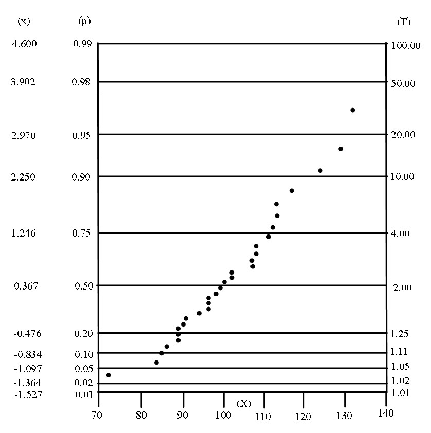
For the plotting we must know \(\mathrm{ x_{ \left[ .367n \right] +1}^{̓}=x_{12}^{̓}=96 }\) and \(\mathrm{ x_{ \left[ .692n \right] +1}^{̓}=x_{21}^{̓}=108 }\) and so the plot in the statistical choice modification of Gumbel probability papers gives the graph Figure 17.1 that follows, agreeing with the use of the Gumbel model.
Figure 17.1. Plot of maximum wind speed at Lisbon (1941-70)
b. Analytical choice of the model:
Once having seen a general trend for the interpretation of data as (approximately) described by the Gumbel distribution, let us confirm (or reject) it by analytic study.
The ML estimators of \(\mathrm{ \left( \lambda , \delta \right) }\) are
which is in the acceptance region for the asymptotically normal distribution of \(\mathrm{ \hat{V}_{n}/\sqrt[]{n~ \hat{\sigma} _{0}^{2}} }\), thus confirming the exploratory analysis. For the value of \(\mathrm{ \hat{V}_{n}/\sqrt[]{n~ \hat{\sigma} _{0}^{2}} =-1.21 }\), obviously, we do not need to go to the refined bounds which are, for \(\mathrm{ \alpha =.05 }\) and to the order \(\mathrm{ O ( n^{-1} ) }\), \(\mathrm{ b_{30}=-~1.71 }\) and \(\mathrm{ a_{30}=2.91 }\), confirming the decision.
It would be useful to divide the sample into two parts (about 2/3 and 1/3) and confirm the results.
To a certain extent this was done in the papers by Tiago de Oliveira (1981) and Fransén and Tiago de Oliveira (1984): in the former, data for greatest ages of death for men and for women in Sweden are studied for the years 1905/1958, and in the latter corresponding data for a larger set of years (1905/1970); and the results are coherent.
Other cases have been considered in the paper by Fransén and Tiago de Oliveira (1984) and can be considered as exercises. We will only follow another case leading to a different decision — the choice of the Fréchet distribution.
It would also be useful to read Whitmore et al. (1987) where data for maximum wind speeds are analysed for Canada.
3 . Flood discharges of the North Saskachevan River at Edmonton
In this case we consider not only the raw data but, as a consequence of the rejection of the Gumbel distribution as a possible model, their logarithms. The ordered raw data, for a period of 47 years in \(\mathrm{ 1000~ft^{3}/s }\), is[2]
which as \(\mathrm{ x_{max}=185.560 }\), \(\mathrm{ x_{med}=~40.400 }\) and \(\mathrm{ x_{min}=~19.885 }\) takes the value \(\mathrm{ Q_{47}=7.0757982~ }\); we have \(\mathrm{ \beta _{47,0}=2.0317188 }\) and of \(\mathrm{ \alpha _{47,0}=.7417784 }\). So
thus rejecting the acceptance of the Gumbel distribution as an approximate model.
b. Analytical choice of the model:
The values of \(\mathrm{ ( \hat{\lambda} ,\hat{ \delta} ) }\) are \(\mathrm{ \hat{\lambda}=38.151 }\) and \(\mathrm{ \hat{ \delta }=17.740 }\), thus giving \(\mathrm{ \hat{ V}_{47}=37.77531 }\) and then \(\mathrm{ \hat{ V}_{47} /\sqrt[]{2.09797 \times 47}=3.804 }\), outside the acceptance region of the asymptotically normal distribution of \(\mathrm{ \hat{ V}_{47}/\sqrt[]{n \hat{\sigma }_{0}^{2}} }\) at a level even smaller than 2%. But this value leads to the Fréchet distribution in the statistical choice procedure.
c. Analysis of the logarithms of raw data:
The value of \(\mathrm{ \left( Q_{47}- \beta _{47,0} \right) / \alpha _{47,0} }\) and of \(\mathrm{ \hat{V}_{47}/\sqrt[]{2.09797 \times 47} }\) suggest the relevance of trying the Fréchet distribution. Denoting by \(\mathrm{ ’x=log~x }\) we get \(\mathrm{ ’x_{max}=5.2234 }\), \(\mathrm{ ’x_{med}=3.6988 }\) and \(\mathrm{ ’x_{min}=2.9900 }\) and \(\mathrm{ ’Q47=2.1509594 }\) and so \(\mathrm{ \left( ’Q_{47}- \beta _{47,0} \right) / \alpha _{47,0}=.1607495 }\), which leads us to accept the Gumbel distribution for \(\mathrm{ log~x }\) and thus suggests the use of the Fréchet approximation.
Let us confirm this analytically. We have \(\mathrm{ \hat{ ’ \lambda }=3.5489 }\), \(\mathrm{ \hat{ ’\delta} =.3963 }\), \(\mathrm{ \hat{ ’V}_{47}=-1.95849 }\) and \(\mathrm{ \hat{ ’V}_{47}/\sqrt[]{2.09797 \times 47}=-1.197 }\), thus leading to the acceptance of Gumbel distribution for the logarithms of raw data and thus the Fréchet distribution for raw data, as seen in (b).
4 . Flood discharges of the Fox River at Berlin and Wrightstown
In this analysis we will use flood data the Fox river at two points of its course: Berlin (upstream) and Wrightstown (downstream), both in Wisconsin, USA[3]
The set of data of \(\mathrm{ n=33 }\) pairs of observations is given in Table 17.3.
Table 17.3
Year
Berlin
Wrightstown
Year
Berlin
Wrightstown
1000 ft3/s
1000 ft3/s
1000 ft3/s
1000 ft3/s
1918
6.05
16.3
1935
4.34
11.1
1919
2.67
13.1
1936
4.34
6.3
1920
5.15
16.6
1937
3.26
13.5
1921
2.45
14.2
1938
6.19
18.0
1922
5.95
20.1
1939
4.91
18.2
1923
6.05
13.7
1940
4.72
17.5
1924
4.02
15.5
1941
3.54
16.6
1925
2.52
8.3
1942
2.74
19.8
1926
3.44
9.1
1943
5.08
21.3
1927
3.17
13.3
1944
2.29
10.8
1928
5.92
15.1
1945
3.46
15.8
1929
6.62
20.6
1946
6.90
21.3
1930
3.00
6.6
1947
3.16
11.0
1931
1.14
3.1
1948
4.54
10.3
1932
1.91
9.9
1949
2.00
6.4
1933
2.60
8.9
1950
4.63
10.9
1934
1.91
6.7
We can, evidently, expect dependence between the yearly flood discharges at Berlin (B) and Wrightstown (W). The graphs on the probability paper show that the Gumbel distribution fits well to the observed marginal flood discharges. The ML estimators are \(\mathrm{ \hat{\lambda }_{B}=3.21070, \hat{\delta} _{B}=1.33880 }\), \(\mathrm{ \hat{ \lambda} _{W}=10.89643 }\) and \(\mathrm{ \hat{ \delta} _{W}=4.61371 }\) and the empirical Kolmogoroff-Smirnov statistics are \(\mathrm{ KS_{B}=.07462 }\) and \(\mathrm{ {KS}_{W}=.09957 }\) with \(\mathrm{ \sqrt[]{n}~{KS}_{B}=.429 }\) and \(\mathrm{ \sqrt[]{n}~{KS}_{W}=.572 }\) accepting thus the Gumbel model for the margins. Evidently the better analysis is to use the \(\mathrm{ \hat{V}_{n} }\) statistics for each margin.
The elements for our statistical decision are the values of the estimated correlation coefficient \(\mathrm{ \rho ^{*}=.693, }\)the medians \(\mathrm{ \tilde{\mu} _{B}=3.54 }\) and \(\mathrm{ \tilde{ \mu} _{W}=13.5 }\) and the number \(\mathrm{ N=24}\) of pairs \(\mathrm{ \left( x_{i},y_{i} \right) }\) such that \(\mathrm{ x_{i}> \tilde{ \mu} _{B} ~ }\) and \(\mathrm{ y_{i}> \tilde{ \mu}_{W} }\) (first quadrant) or \(\mathrm{ x_{i}< \tilde{ \mu} _{B} }\) and \(\mathrm{ y_{i}< \tilde{ \mu}_{W} }\) (third quadrant). This value of \(\mathrm{ N }\) is not coincident with the total of the first and third quadrants (22) given in Gumbel and Mustafi (1967) because the authors, instead of computing the medians directly from the sample, estimate the margin parameters and from them compute estimated medians. The test of independence, as \(\mathrm{ \sqrt[]{n}~ \rho ^{*}=\sqrt[]{33} \times .693=3.981 }\)is larger than the values \(\mathrm{ \lambda _{0.05}=1.64 }\) and \(\mathrm{ \lambda _{0.01}=2.33 }\), leads to rejection of independence at level 1%. Consequently we will have to estimate \(\mathrm{ \theta }\).
Let us consider first the mixed model. As the larger value of \(\mathrm{ ~ \rho ^{*} }\) in the mixed case is 2/3, we have no point estimator of \(\mathrm{ \theta }\) by this method (the best being evidently \(\mathrm{ \theta ^{*}=1 }\), allowing for sampling errors).
The relation \(\mathrm{ p^{**}=p_{M} \left( \theta ^{**} \right) =2^{-2+{ \theta ^{**}}/{2}}=\frac{N}{2~n}=\frac{24}{2 \times 33}=.36364 }\) gives \(\mathrm{ \theta ^{**}= 1.0 81 }\) and thus is not solvable for \(\mathrm{ \theta ^{**} }\) as we should have \(\mathrm{ 0 \leq \theta ^{**} \leq 1 }\); also note that the maximum value of \(\mathrm{ p_{M} \left( \theta \right) }\) is \(\mathrm{ p_{M} \left( 1 \right) =.35355<\frac{24}{2 \times 33}=.36364 }\). The mixed model must therefore be rejected.
Consider now the logistic model. As \(\mathrm{ 0 \leq \rho _{L} \left( \theta \right) \leq 1 }\) the equation \(\mathrm{ \rho _{L} \left( \theta ^{*} \right) = \theta ^{*} \left( 2- \theta ^{*} \right) =.693 }\) can be solved giving \(\mathrm{ \theta ^{*}=446 }\). As \(\mathrm{ p_{L} \left( \theta \right) =2^{-2^{1- \theta }} }\), the equation \(\mathrm{ p^{**}=p_{L} \left( \theta ^{**} \right) =\frac{N}{2n}=.36364 }\) gives \(\mathrm{ \theta ^{**}=.4546 }\), which is close to the previous estimate, justifying to a certain extent the use of the logistic model.
Note that this is a margin (location-dispersion) parameter-free approach. As said, Gumbel and Mustafi (1967) used estimators of the margin parameters and computed the estimated reduced difference, comparing it, by the Kolmogorov-Smirnov test, with the logistic and confirming the suggestion to use the logistic model as an approximation.
Recall that estimation of the margin parameters involves as yet unsolved problems with the use of the Kolmogorov-Smimov test, although it gives a hint for the logistic model, as stated.
The 5% asymptotic confidence interval is given by
\(\mathrm{ \vert p_{L} \left( \theta \right) -p^{**} \vert \leq 1.96\sqrt[]{p^{**} \left( .5-p^{**} \right) }/\sqrt[]{n} }\) which is, in our case,
\(\mathrm{ \vert p_{L} \left( \theta \right) -.36364 \vert \leq .07598~or~.28766 \leq p_{L} \left( \theta \right) \leq .43962 }\) and so
\(\mathrm{ .154 \leq \theta \leq .754 }\), a very large (asymptotic) confidence interval.
Let us now consider the biextremal model. The equation \(\mathrm{ \rho _{B} \left( \theta ^{*} \right) =.693 }\) gives \(\mathrm{ \theta ^{*}=.55 }\). The solution from \(\mathrm{ p_{B} \left( \theta ^{**} \right) =2^{-2+ \theta ^{**}}=.36364 }\) is \(\mathrm{ .54 1 }\); the approximate confidence interval for the significance level 5% is \(\mathrm{ \vert p_{B} \left( \theta \right) -.36364 \vert \leq .07598~is~.202 \leq \theta \leq .814 }\).
For the Gumbel model the equation \(\mathrm{ \rho _{G} \left( \theta ^{*} \right) =.693 }\) gives \(\mathrm{ \theta ^{*}=.723 }\) and the confidence interval from \(\mathrm{ p_{G} \left( \theta \right) =p_{B} \left( \theta \right) }\) is also \(\mathrm{ .202 \leq \theta \leq .814 }\), which suggests that the Gumbel model is not appropriate to this problem, the solution of \(\mathrm{ \rho \left( \theta ^{*} \right) =.6846 }\) being close to the upper bound of the confidence interval; in fact the model arises naturally in questions connected with failures. A simple check can be the estimation of \(\mathrm{ \theta }\)from the use of Kendall’s \(\mathrm{ \tau_{G}= \theta / \left( 2- \theta \right) }\).
The question of discriminating between models, as for the remaining ones (logistic, biextremal) in this example is, as yet, an unsolved problem. Here, though, the solution is simple.
As in the biextremal model we have for the reduced values \(\mathrm{ Y=X }\) with probability \(\mathrm{ \theta }\) and \(\mathrm{ Y>X }\) with probability \(\mathrm{ 1- \theta }\), we can expect that, roughly, \(\mathrm{ n~ \theta }\) observations \(\mathrm{ \left( x_{i},y_{i} \right) }\) should be in a straight line\(\mathrm{ y=ax+b }\) and rest should be such that \(\mathrm{ y>ax+b }\). In our case, as \(\mathrm{ \theta ^{*}=.541 }\) and \(\mathrm{ n= 33 }\) we should have roughly \(\mathrm{ {.541} \times 33 \approx18 }\) points in a straight line; the scatter diagram given in Gumbel and Mustafi (1967) shows immediately that this is not the case. Of the four models considered, the only one not yet rejected is, for the moment, the logistic. Also the plotting of estimated reduced differences on the logistic paper, given also in Gumbel and Mustafi (1967), speaks in favour of the logistic model.
The application of the strip method — see Posner et al. (1969) referred to in Chapter — to the logistic model as a flood model for the Fox River confirms its usefulness.
It should be remarked here that if we expect bivariate models to be absolutely continuous here, as in other cases, the logistic model seems to be a good candidate. Also, as shown in Tiago de Oliveira (1987) the discrepancy between the logistic and \(\mathrm{ \left( 2,N \right) }\) natural model is small and not easily seen for such small samples. The intrinsic estimation will also not give large discrepancies.
5 . Footnotes
[1]. The author thanks the Portuguese Institute for Meteorology and Geophysics for having kindly supplied the data.
Fransén, A. and Tiago de Oliveira, J., 1984. Statistical choice of univariate extreme models, part II, in Statistical Extremes and Applications, Tiago de Oliveira, J, ed., 373-394, D. Reidel, Dordrecht.
Tiago de Oliveira, J., 1981. Statistical choice of univariate extreme models, Statistical Distributions in Scientific work, 6, G. P. Patil ed., 6, 367-387, D. Reidel, Dordrecht.
5.
Tiago de Oliveira, J., 1987. Comparaison entre les modeles logistique et naturel pour les maxima et extensions, C. R. Acad. Sc. Paris, t. 305(1), 481-484.
6.
Van Montfort, M.A.J., 1970. On testing that the distribution of extremes is of type I when type II is the alternative, J. Hydrology, 11, 421-427.
7.
Whitmore, G. A., et al. 1987. Case studies in data analysis, nº 5. Canad. J. Statist., 15, (4), 311-337.