Keywords

building extraction , Ensemble modeling , NDVI , PCA , model stacking

1 . INTRODUCTION

Building extraction from the satellite imagery has been a very challenging application in geographical urban data development. In the recent years, increased availability of quality (both spectral and spatial) remote sensing satellite imagery have filled up the void in technology and have given researchers the ability to develop algorithms for building extraction from the very High-resolution satellite imagery. Spatial resolution forms a very important part in the identification of buildings to perform building extraction and detection.

Building detection using the satellite imagery has significant applications in land use change mapping, urban planning, disaster risk assessment, urban space use mapping. Researchers across the globe have developed many indices for various feature extraction including urban, land cover, vegetation, water bodies. Spectral-based indices (Xu, 2008) are the most commonly used for urban structure extraction (He et al., 2010). Examples include Normalized Difference Built-up Index (NDBI), Normalized Difference Vegetation Index (NDVI), Soil Adjusted Vegetation Index (SAVI) and Modified Normalized Difference Vegetation Index (MNDVI), etc., (Ramachandra et al., 2012; Ramachandra et al., 2016; Bharath et al., 2018). But, spectral indices couldn’t solely be used for extraction of buildings because of a significant amount of spectral mixing and heterogeneity of pixels of various land cover 

types of urban scenario mainly, water bodies, built-up, barren land, as a result, reduces the accuracy of extraction (Sinha et al., 2016). To overcome these issues, two methods have been used: (i) classification involving various algorithms at pixels and object levels and (ii) enhanced spectral indices for buildings and then thresholding.

In machine learning, spectral indices can be used as attributes in identifying the pixels containing the building in complement with the spectral bands. Hence, the algorithms are trained with the values in various attributes and their labels from which it learns those small intricacies of the relations between attributes increase the classification accuracies. In this study, NDVI is used to complement Principal Component Analysis (PCA) and generated multispectral bands are used for the machine learning process.

1.1 Machine Learning and Applications in Building Extraction

Last decade machine learning has been widely used in remote sensing, that involved an enormous amount of data. Machine learning is based on the process of designing of algorithms that can learn from the data provided by the user for a particular phenomenon under analysis (Lary et al., 2016). One of the applied areas of application is the extraction of the building edges and heights. Extraction of the building is a complex procedure because of homogeneity of the spectral properties with other urban objects in the satellite imagery. Machine learning approach for building extraction from Very High Resolution (VHR) satellite image is quite helpful as it takes various predictors variables for a final prediction of presence or absence of a building. Using machine learning many studies have tried to develop automatic building detection algorithms (Dahiya et al., 2013). These algorithms considered building as objects and then segmentation is used to create the image object using the spectral properties, texture, or the shape of the image object. The possibility of incorrect extraction of features was observed in a complex urban scene with decrease in accuracy.

Studies have also used deep convolution neural networks and residual networks along with guided filters for building extraction and showed outstanding performance in building extraction which results in high computational demand (Xu et al., 2018). Similarly, in Yuan (2016) simple convolution neural network was used for building extraction which showed higher accuracies in the developed urban environment but accuracies degraded when applied to rural and suburban areas which showed that machine learning can play an important role in building extraction process giving significant accuracies. In Aytekın et al. (2012), genetic algorithm for building extraction was used for a multispectral image with pan-sharpening, showed promising results in building extraction with complete rooftop extraction of the buildings.  Also extracted some complete barren areas as building’s rooftops and is observed that it gave higher accuracies when both spatial and spectral properties were considered.

There has been various studies such as Chen et al. (2018) that used machine learning methods for classification of buildings. Support Vector Machine (SVM), Random Forests (RF) and AdaBoost were methods used to extract building data and reported that SVM provided a good accuracy.  It is observed that SVM proved to be very good in building extraction but intermixing of pixels with surrounding urban areas was observed. Further, Dornaika et al. (2016) highlighted building detection using image segmentation and descriptors on aerial orthophoto. In this study segmentation of image is performed, after which region descriptors are provided for segments than machine learning is applied which showed higher accuracies. Region descriptors played an important role in the machine learning process as many features are attached to a single label, complementary to one another that are helping in getting greater accuracies. This study drew an inference as increasing attributes for labels the accuracies could be increased. Guo et al. (2016) have used Google Earth imagery using Convolution Nueral Network (CNN) and AdaBoost methods in extraction of building. Studies including Das and Ghosh (2017) and Martin and Vatsavai (2013) showed that ensemble of different models or classifiers generally corrects the errors committed by a single classifier thereby, increasing the accuracies. Ensemble learning was also applied on Hyperspectral imageries that increased their classification accuracies (Wu et al., 2012).

Each of the machine learning algorithms such as (a) SVM, (b) Ensemble and decision tree based as RF, (c) Artificial Neural Networks (ANN), etc., have been extensively used specifically in the extraction of buildings.

1. SVM classifiers work by creating a separating hyperplane between the support vectors that the training pixels and separates two classes in the feature space. The optimization is done by maximizing the margin between the hyperplane and closest support vector or training samples. This works well even with small training data sets when classifying high dimensional data because it only takes into considerations those training samples that are close to the margin, called support vectors and thus has seen few applications in an urban context (Waske et al., 2009).
2. Random forests algorithm is an ensemble-based machine-learning algorithm that uses multiple classifiers to generate multiple outputs to vote for better outcome. This is comparatively a very recent development and application are still very few (Breiman, 2001, Gislason et al., 2006). RF uses each individual classifier and then uses each of them to train on a subset of training data and the result is the mode of the classes of the individual decision trees with the goal of decreasing the variance. The training samples are divided by using the bagging technique and the split in each node is based on a test rule.
3. Artificial neural networks are based on the bioinformatics that mimics human brain structure and features to gain a perception of a phenomenon under study. ANN’s ability to provide better outputs even when relationships between various variables are not known is an added advantage and is capable of establishing connections between predictor variables efficiently. ANN has been adopted in various studies in Built-up extraction (Lari and Ebadi, 2007; Patel and Mukherjee, 2015; Sahar et al., 2006).
4. Finally, ensemble modeling runs two or more related but different predictive models then fuses the predictions for a single score (Gunes et al., 2017). Model stacking is used in ensemble learning in order to improve the accuracy of prediction using base learners. Stacking is primarily an ensemble based meta-learning technique that combines information or predictions from different predictive models to generate a new model. Generally, the stacked model performs better from the individual learners due to its nature of smoothing and the ability to predict when the base models perform well and discredit it when it performs poorly. Studies have showcased ensemble based learning for prediction of missing data in a time series data from multiple learning modules ( Das and Ghosh, 2017). Further studies like  Puttinaovarat and Horkaew (2017) have used a fusion of multiple outputs from different classifiers for building extraction which resulted in a higher overall accuracy of extraction.

In this study, we have used gradient boosting as a method of ensemble learning, as proved to provide better accuracy. Based on above discussion we propose an ensemble based extraction algorithm in which, various algorithms or base learners i.e. SVM, RF, ANN are combined for a final extraction result. This method has the capability of correctly classifying misclassified pixels increasing the extraction and detection accuracy. 

Thus, considering all these aspects, the main objective of this study is to find out the potential of three prominent machine learning algorithms e.g. SVM, RF, ANN in automatic building extraction for the urban area from very high-resolution satellite datasets.

We have been evaluated the potential of an ensemble method using stochastic gradient boosting for building prediction in the homogeneous and heterogeneous distribution of building structures and at different spatial resolution.

2 . DATA BASE

In this study, high resolution and very high-resolution satellite data were used for building extraction. Building extraction in images is a difficult task due to non-linearity of the building structure and lack of homogeneous arrangement of buildings. Spatial resolution is an integral part of the extraction process and is considered as one of the comparative assessment indicators for successful extraction. Resourcesat-2 LISS-IV data at 5.8m spatial resolution (Figure 1) was  used to  study  and  evaluate  the  behavior  of  algorithm at a medium spatial resolution with non-linearity and  heterogeneity  of building structures. Data from  Worldview-2  (Figure  2)  satellite captured at very  high-resolution was provided by  DigitalGlobe  with  a  spatial  resolution  of  0.5m  panchromatic,  2.5m  multispectral  used to study and evaluate the behavior of the algorithm at a highly spatial resolution with high non-linearity of buildings. WorldView-3 (Figure  3)  images  at  a  high  spatial  resolution of 0.4m panchromatic, 1.25m multispectral provided by DigitalGlobe was processed for the analysis as the region has buildings that are linear and homogeneous as tabulated in Table  1.

Figure 1: Resourcesat-2 LISS IV

Figure 2: Worldview-2

Figure 3: Worldview-3

3 . METHOD

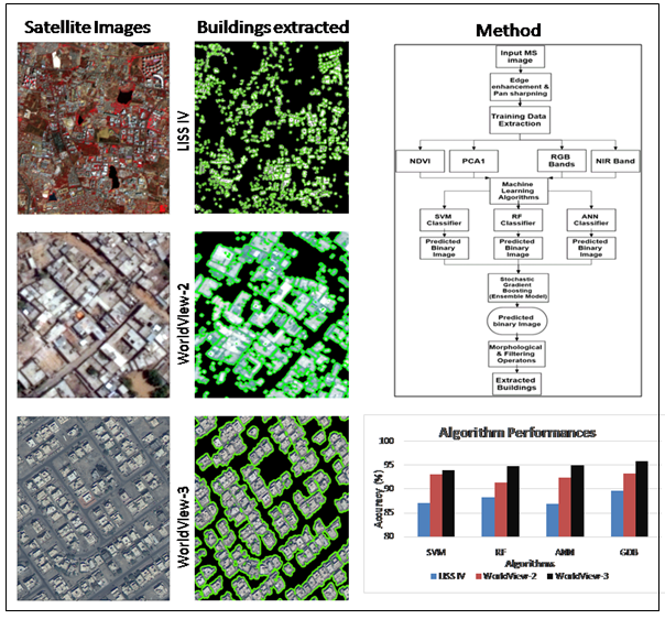
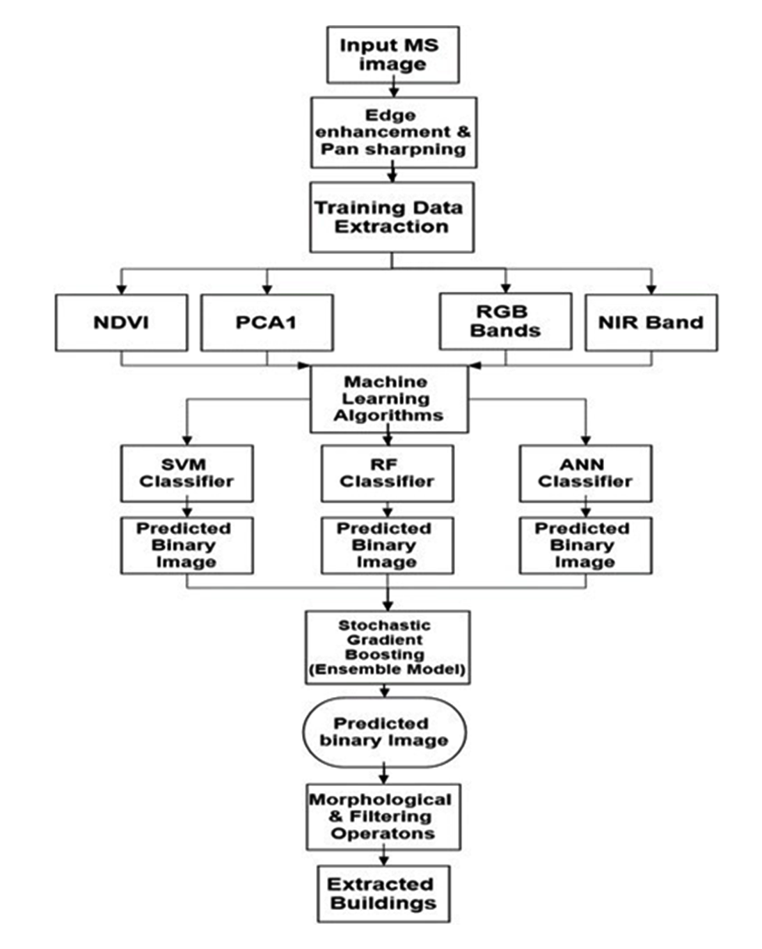
Methods used for building extraction using machine and ensemble learning are follows the process shown in Figure 4.

Figure 4: Process of building extraction

3.1 Data Preprocessing and Preparation

Raw data sets are corrected for geometric and radiometric errors induced due to sensor distortions or due to the platform and atmospheric distortions.  For radiometric corrections, histogram equalization was performed that maximizes the contrast of the data by applying a nonlinear contrast stretch that redistributes pixels so that there is equal number of pixels under each value within the range. Pan-sharpening was performed for the imagery to increase the spatial resolution for the extraction of buildings. Projective pan-sharpening was performed on the imagery as it gives much better results as it preserves the color of the imagery as described in (Lindgren and Kilston, 1996).

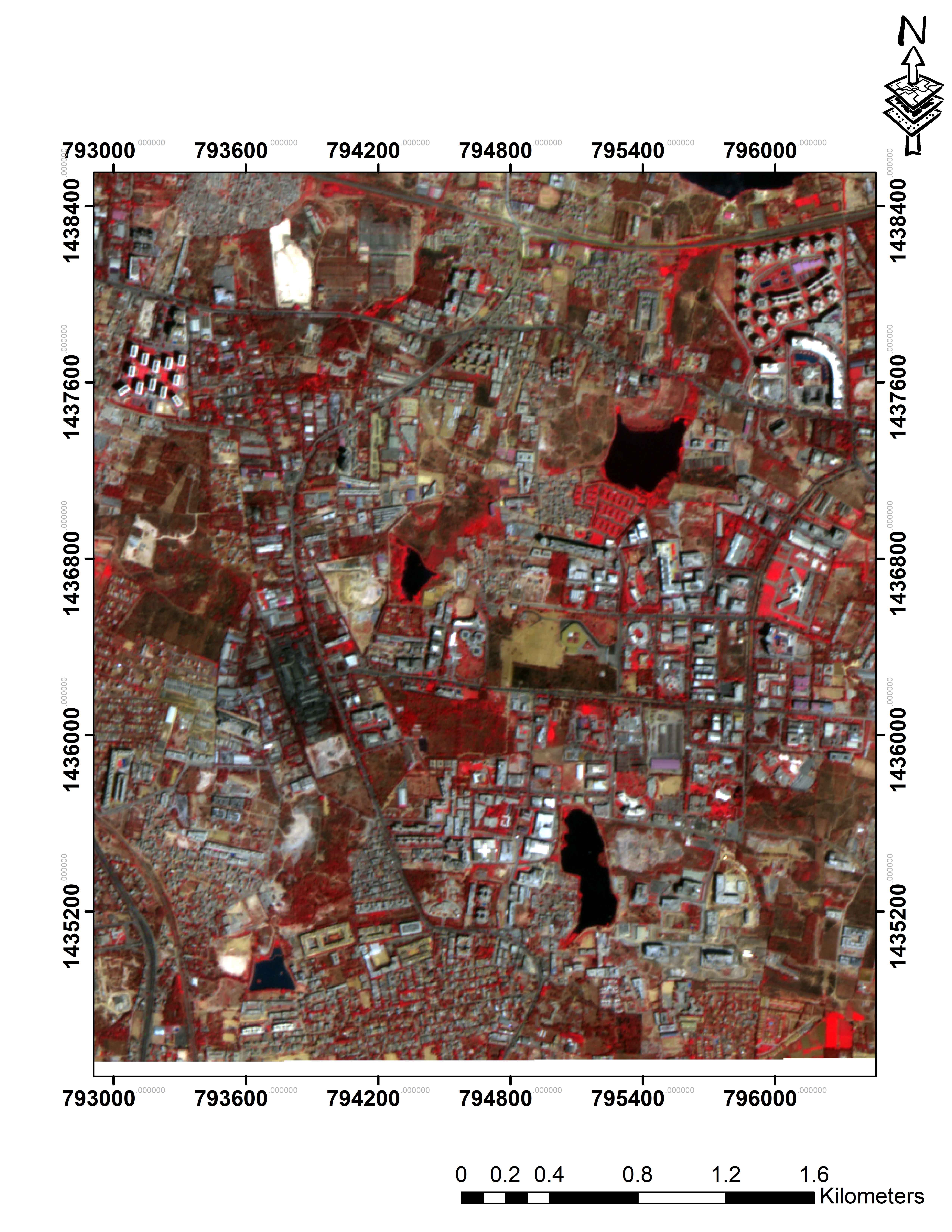
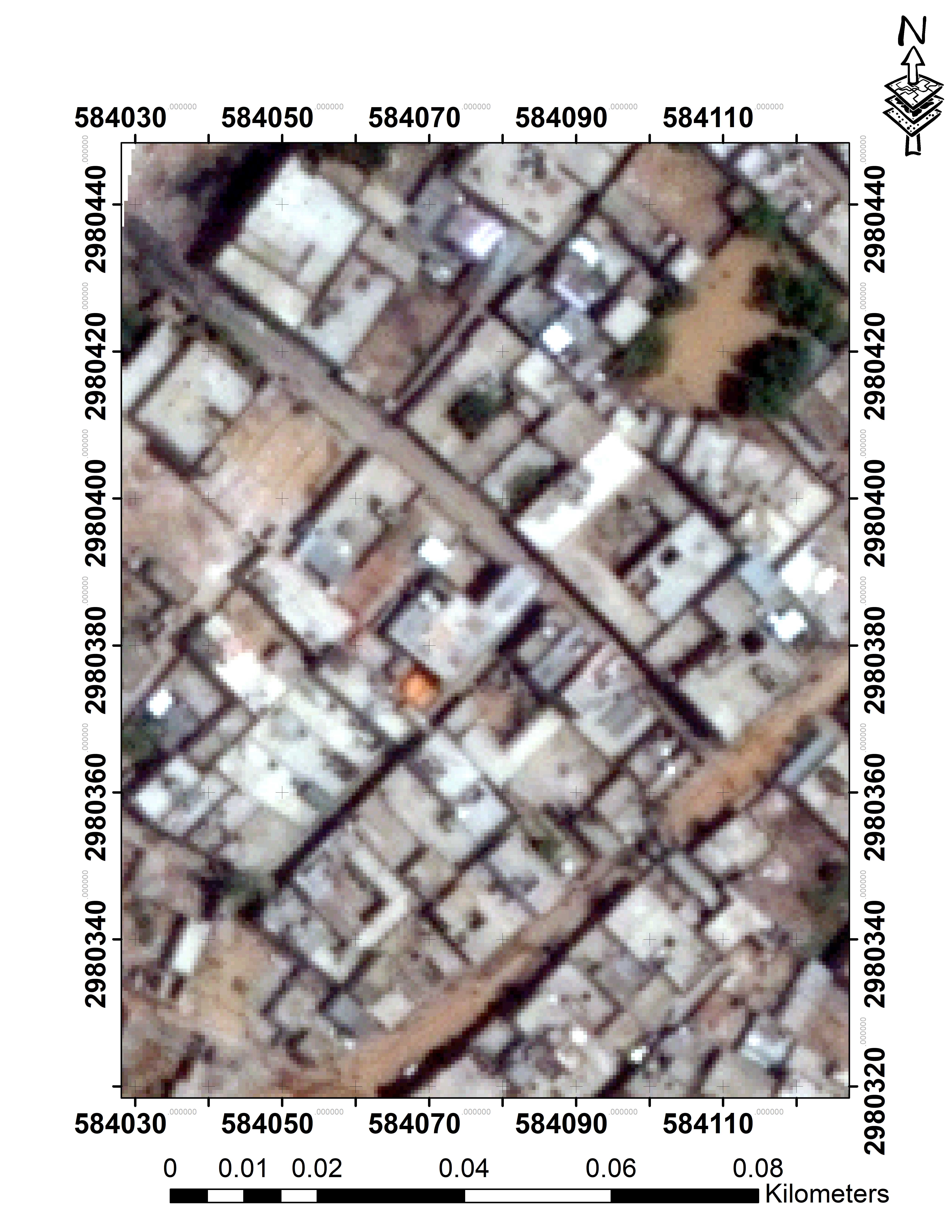
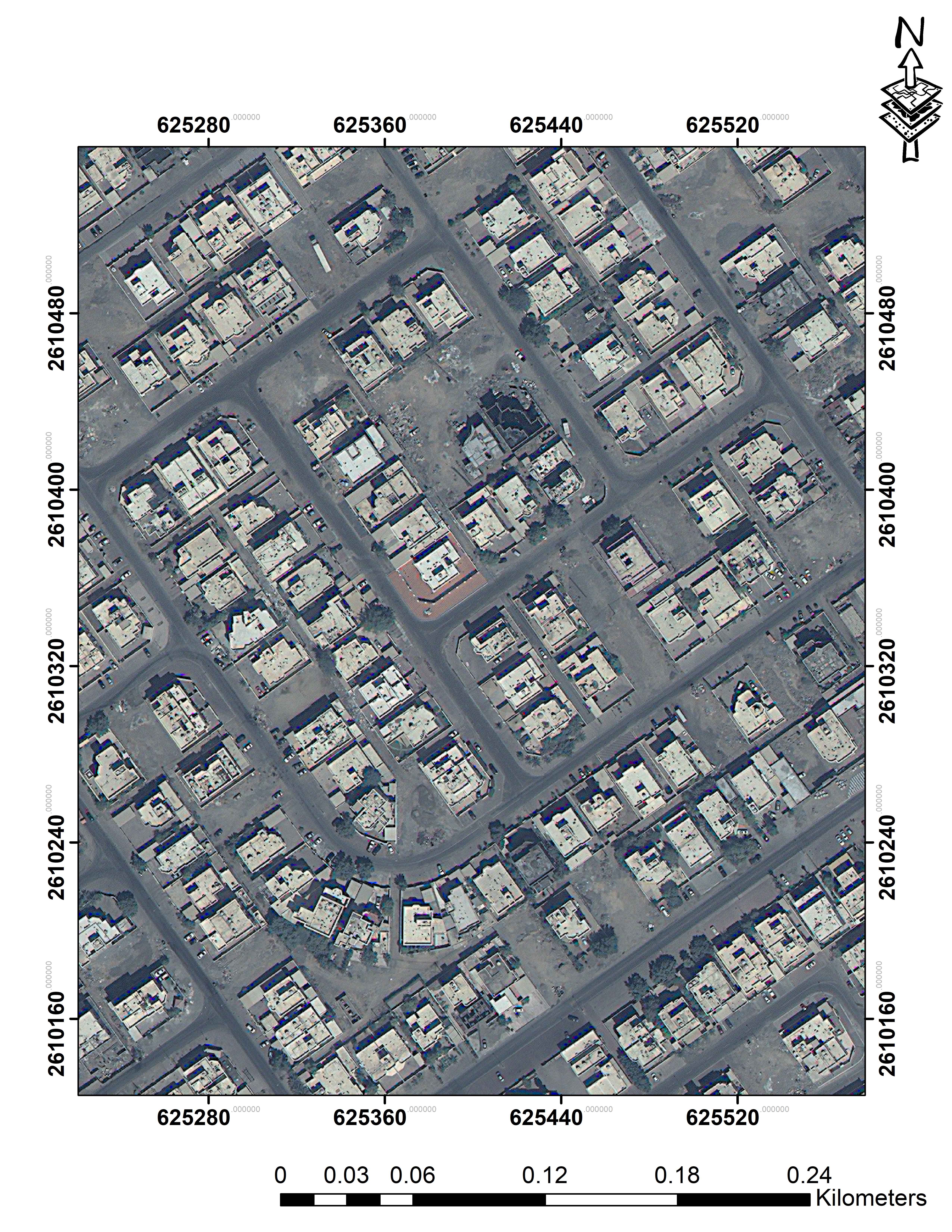
Edge enhancement is performed on the image to enhance the edges in imagery with a sharp decrease and a sharp increase in intensity value of pixels to increase the probability of building extraction. This pan-sharpened and edge enhanced image are used to calculate the spectral indices and principal component. Only edge enhancement was performed on the LISS-IV imagery while both edge enhancement and pan-sharpening of multispectral bands of WorldView-2 and WorldView-3 were performed using their respective panchromatic bands of 0.5m and 0.4m resolutions.

3.2 Spectral Indices and PCA of Satellite Imagery

NDVI (Bhandari et al., 2012) is calculated using the pan-sharpened and edge enhanced imageries. NDVI has been used specifically for monitoring of vegetation and land cover studies. It basically measures the amount of chlorophyll present in the plants. The plant absorbs the infrared region of the spectrum than in the red region so the contrast between the two is used to build an index as described in equation (1). Different land cover has variations in NDVI values. Vegetation has very high value that decreasing with decreasing chlorophyll content. Buildings also have specific NDVI value based on the scene characterizes, for the study area it varies between -0.02 and 0.6. NDVI is calculated for the dataset which is used as an attribute for input data to machine learning algorithm for extraction of buildings.

NDVI = (NIR − RED) / (NIR + RED)               (1)

PCA (Estornell et al., 2013) was performed based on the Infrared (IR), Red, Green and Blue (RGB) which gives various principal components as with decreasing variance and decreasing content of information. First principal component was selected as it has high variance.

Figure 5. (A) NDVI and (B) PCA1

3.3 Machine Learning Algorithms for Building Extraction from Very High-Resolution Satellite Imagery

After calculation of NDVI and PCA 1, each of the following algorithms was systematically used along with data input as building and non-building that are manually digitized. This manually digitized data is divided into a training dataset and test dataset (Verticale and Giacomazzi, 2008) in 7:3 ratio. Training data is used for training the algorithms and test dataset as validation data and is used for accuracy assessment of the algorithms.

3.3.1 Support Vector Machine Classification

SVM  is a type of non-parametric supervised machine learning algorithms work by creating a separating hyperplane in a multi-dimensional feature space and that maximizes the orthogonal distance between hyperplane and the support vectors  (Chapelle, 1998). Optimization is performed by maximizing the margin between the hyperplane and closest support vector or training samples. This works well even with small training data sets when classifying high dimensional data because it only takes into considerations those training samples which are close to the margin, which is, therefore, called support vectors. Training dataset consists of points x_i ∈ R^N, i = {1,…….,l,}. Where each data point belongs to one of the two class given by class labels y_i = +1 or y_i = -1.

The algorithms work such that it draws decision boundaries or hyperplanes w . x + b, where the decision rule function w . x_i + b > = 0 than, y = +1 and w . x_i + b < = 0 than, y = -1, where y is the label for the data point x_i.. Optimization of equation (2) is used in generalizing the optimal hyperplane.

\(min ({1 \over 2 } \| w^2 \|+c\sum_{i=1}^{l} \xi_i)\)                                     (2)

Subject to y_i (w^T.x_i + b) >= 1 – ξ_i , ξ_i >= 0

Here, ξ_i are positive slack variable and C > 0 is the regularization parameter or cost for any miscategorization errors.

If training datasets are linearly separable then the data points could be separated into two classes without error using a linear hyperplane. Generally, building structures are non-linearly separable cases with high non-linear relationships between the whole dataset and training datasets. Hence, as building distribution in imageries are more to near heterogeneous in nature, we use non-linear kernel functions. In which we exploit the SVM classifier radial basis function to map those data points in its feature space to higher dimensional feature space where the data points are separable. SVM linear classifiers find an optimal hyperplane using dot product between data point vectors (equation 3) and decision function shown in (equation 4).

  \(K(\overrightarrow{x}{_i},\overrightarrow{x}{_j})= {\overrightarrow{x}{_i}}{^T},\overrightarrow{x}{_j}\)                                                  (3)

\(f(\overrightarrow{x})=sign(\displaystyle\sum_i a_iy_iK(\overrightarrow{x}{_i},\overrightarrow{x})+b)\)                    (4)                                                     

where, α_i is a Langrage multiplier which is non-zero for support vector.

Kernel function as shown in equation (5) is then used to project every data point x_i to higher dimensional space via transformation is used.

\(K({\overrightarrow{x}{_i}}{^T},\overrightarrow{x}{_j})= \phi({\overrightarrow{x}{_i}}), \phi(\overrightarrow{x}{_j})\)                                (5)

where, \(wT.\varphi(X_i)+b\)  is the separating hyperplane in higher dimensional space, it is transformed to a decision function equation (6), non-linear decision function, after optimal α_i is found, a sample x_i can be classified by finding out the side of hyperplane it lies in the new feature space (Waske et al., 2009).

\(f(\overrightarrow{x})=sign( \sum_i a_iy_i (\phi({\overrightarrow{x}{_i}}). \phi(\overrightarrow{x}{}))+b)\)          (6)

As per the literature, there are mainly two groups of kernel function: Polynomial kernel and Radial basis kernel. In this study radial basis function (equation (6)) is used because it could classify points when the relationships between the labels of the class and attributes follow a non-linear pattern. It could be helpful in identification of buildings which generally follow a non-linear or heterogeneous heterogeneous arrangement. SVM and Radial basis function (RBF) (equation (7)):

\(K(x,\overrightarrow{x}{_j})= exp{(\| x-x_i\|) \over2\sigma^2}\)                         (7)

Thus, the process of building extraction using SVM is performed using 5 major steps:

1. The training data with values from various attributes are scaled and prepared for the input into the algorithm.
2. To find the best-fit C and σ for the training dataset tuning was performed,
3. RBF as kernel is used with the best C and σ on the training dataset to obtain a model.
4. The model is used to predict the test dataset and accuracy is calculated as previously described
5. After achieving a good accuracy, the model is used for prediction on the imagery. This also includes recoding the image as 0, 1, 0 for absence and 1 for presence.

3.3.2 Random Forests Classification

Random forests (Horning, 2010) machine learning algorithm is an ensemble-based supervised machine learning algorithm which uses multiple decision tree (DT) classifiers to create a forest and generate multiple outputs to vote for a final result using majority vote. RF works by first creating ‘k’ decision trees using the training dataset and the feature space by a technique called Boosting Aggregating or Bagging, which randomly selects and divides with replacement into bootstrap samples. Hence, there are samples those are not in the bootstrap samples are also called out-of-bag (OOB) samples, these samples are used for misclassification errors and variable importance called OOB error and then, it selects attribute features from given M attribute features for building decision trees. The best split at each node is chosen based on Gini impurity or information gain method, where, this is called Random subspace method. After the ‘k’ decision tree predicts their output, the prediction by the majority of the trees is chosen by RF as the final prediction.

If there are n samples and with feature vector x_i with labels y_i, where, {i=1, ……., n}, therefore, Data (D) ={ (x_i,y_i), ……….. , (x_n,y_n)}, Feature vector (x_d)= (x_d1,…….., x_dr),

Many trees are built, in which each tree has a node with binary decision values, the division of tree continues until it has only one class and at each node feature (x_i) and threshold (a), which are constant is chosen with minimum Gini criterion or impurity (Joelsson et al., 2005), if there is a subset of sample S, with two class C₁ and class C₂ then, variation g(S_j), j is number of samples in S, as shown in equation (8),

\(g(S_j) = \displaystyle\sum_{i=1}^{2} \hat{P}(C_i\mid S_j) (1-\hat{P}(C_i\mid S_j))\)                 (8)

Where, \( \hat{P}(S_j) \)  proportion of S_j in S, \( \hat{P}(C_i\mid S_j)\)  is proportion of S_j in C_i. Variation \(g(S_j) \) = Gini index = G under certain conditions. If each tree built is considered as weak classifier, then ensemble of weak classifiers is as complied by equation (9).

\(h=\{ h_1(x), \dots \dots .., h_k(x) \}\)                                  (9)

\( \hat{h}(x)= {1 \over k} \hat{h_j} (x)\)                                                     (10)

Where, \( \hat{h_j} \) (equation (10) ) is a weak classifier or tree based on subset of S, for each tree we estimate the error on the unused data, averaging these errors give us the OOB (out-of-bag) error estimate.

3.3.3 Artificial Neural Networks Classification

ANN consists of a network of connections; in which the neurons work as computational units. In a feed-forward neural network, a bias node is added to each layer, a neuron that has a constant output and for each neuron from the input layer to the output layer, a weighted average of input is calculated then, activation function is applied which contains the neuron firing rules. There are various types of activation functions. They introduce non-linear properties into the network so, that they give it the ability to approximate more non-linear distribution (Lek et al., 1996) of data which is in case of building extraction. In this study in the feedforward network, we use a sigmoid activation function, with two input, a hidden layer and an output layer with two classes (building and non-building) and uses BFGS (Broyden–Fletcher–Goldfarb–Shanno) algorithm (Ibrahim et al., 2014) for optimization of the network instead of back propagation.

Training dataset consists of input Xp, p = {1,., i,}. It calculates the weighted average (as shown in equation (11) and sigmoid activation function (equation (12)) is used by the network and Y_j is the output.

   \(Y_j= \sum_{i=1}^{p} (W_{ij}X_i+b)\)                  (11)         

  \(Y_j= {1\over 1+exp (-v_j)} \)                                (12)   

The training datasets are prepared and scaled as the requirement of algorithm preferably its converted into the matrix, then a network is built, then the training data is feed into the network. Initially, sigmoid activation function is set to false, random weights are assigned as 0.1 with weight decay rate (decay) of 5^e-4 , and entropy is considered to be true for loss function. Best parameters are obtained using various combinations on the training data, hence builds a network model. Then it is used to predict the test dataset that is used for accuracy assessment. Once validated the model is used for predictions on the satellite imagery that extracts the building pixels to produce an image with building and non-building area.

3.4 Ensemble-Learning Based Model Stacking Approach for Building Extraction

Ensemble learning (EL) uses a group of weak learning algorithms to form a strong learner with greater accuracy than constituent base learners (Choraś et al., 2009). Ensemble modeling is running two or more different predictive models that predict different outputs, on which strong learner makes predictions for a single score. Two types of EL are generally used; One is Bootstrap Aggregating (Bagging) in which it trains each model with a random subset of training data with equal weight to each models output after that final prediction is the majority vote of all the predictions by all the models and another is Boosting (Gunes et al., 2017), that builds model on the training data, then creates second model that tries to correct the error committed by first model, models are added until the training set is predicted correctly. We use Model Stacking in this study in order to improve the accuracy of prediction using base learners which are SVM, RF, ANN and to make predictions on the outputs of the base learners, we use stochastic gradient boosting an ensemble learner.

3.4.1 Advantages of Model Stacking Over Individual Classifiers and Stochastic Gradient Boosting Approach

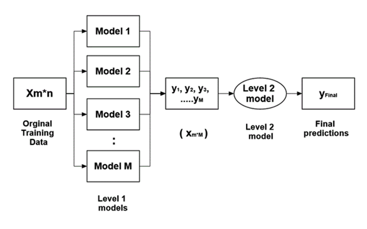
Ensemble modeling approach first uses individual classifiers to make predictions on the training data, and then it uses the predictions from the base learners as input. The output of individual classifiers is then used to train the ensemble learner as illustrated in Figure 6. Generally, the stacked model performs better than the individual learners due to its nature of smoothing and the ability to predict when the base models perform well and discredit it when it performs poorly.  

 

Figure 6. Ensemble modeling

 

Further, after prediction by different machine learning algorithms, outputs are used as input for the second layer of the learning algorithm (Figure 6). Algorithm efficiently combines the predictions of the base learners to form a new model to produce higher accuracy.  In the second layer of the learning algorithm generally models that boost the accuracy of predictions for the complex relationship between input variables are normally used. Stochastic gradient method is one of such non-linear approximating algorithms that help in establishing a complex relationship between variables.

As shown in Figure 6, initial training dataset (X) has m rows or observation and n attributes, for instance, if we consider a number of models used in level 1 is M, M number of predictions and model’s types are trained on the dataset. Then each model gives an output, y_i, Where i= {1, 2….M}.

This forms the training data of the second level consisting of m observations and M attributes. Finally, the second level model is trained on this data (m*M) using gradient boosting, that gives the final predictions.

The aim of the Ensemble Learning Algorithms (Gradient boosting), in this case, is to find and minimize a loss function. We can describe loss as in equation (13) where y_i = i^th target value,  \(y^p_i=i^{th}\) prediction, \(L(y_i -y^p_i)\)  = loss function.

\(loss= MSE= \sum (y_i-y^p_i)^2\)                    (13)           

The predictions should have minimum loss functions or error. It keeps on updating the predictions using gradient descent which moves forward by a learning rate until it finds predictions (equation (14)) with less MSE [Mean Squared Error].

  \(y^p_i=y^p_i+a*\delta \sum (y_i-y^p_i)^2/\delta y^p_i\)              (14)

where, α is learning rate and \( \sum (y_i-y^p_i)\)  is sum of the residuals,

This type of boosting reduces both bias and variance and prevents over fitting of the model 

on the data. Stochastic gradient boosting is a slightly changed version of the gradient boosting in which it uses bagging with boosting which induces randomness in function estimation. Random sub-sample of training data (without replacement) is used at each iteration for the full training data. This subsample is used to fit the base learner and then updates the prediction of the model for iteration. The parameters are tuned and set for optimal performance are loss function, number of iterations, depth of the trees, learning rate and sampling rate or bagging rate. As we now have the output of the three classifiers, the algorithm uses these outputs to build a, model with optimal parametrs, which is used for final building extraction by the ensemble.

3.5 Morphological and Cleaning Operations on Classified Imagery

Morphological and cleaning operations are performed on output image for removal of salt and pepper noise in the image (Kupidura and Jakubiak, 2009). Morphological operators are based on set theory that takes a binary image and a kernel as input and combines using set operators and gives a modified binary image. Open, dilate morphological operations are performed on the image. Clump operator was used to detecting patches of connected pixels. Finally, area filter is applied to the image to remove groups with less than five pixels to get a final extraction of buildings from the imagery. Morphological operations are performed on WorldView-2 and WorldView-3 imageries, while LISS-IV imagery is excluded due to loss of information.

4 . ACCURACY ASSESSMENT AND MODEL PERFORMANCE

Accuracy assessment is performed to evaluate the correctly represented ground reality in the image (Foody, 2010). Confusion matrix is one of the most used methods of assessment of accuracy from which various types of matrices could be extracted for calculating accuracy and errors. This will also help us to access and analyze the performance of the model in different conditions using test data. The predictions of the model on test dataset will be used for generating confusion matrix, accuracy, kappa, sensitivity, specificity along with two metrics Branch Factor (BF) and Detection Percent (DP) (Lin and Nevatia, 1998).

DP is how many buildings get detected in the image by the algorithms and BF is the how many buildings are found improperly. Generating these metrics requires manual digitization and comparison as explained in equations (15) and (16).

Building detection (DP) rate:

\( DP=100*({TP\over TP+TN})\)                         (15)

Branch Factor \((BF)=100*({FP\over TP+FP})\)   (16)

where, TP = building detected both manually and by the algorithm (sensitivity), TN = Building detected manually, but, not by an algorithm (specificity), FP= Building detected by the algorithm but, not manually. BF is how many buildings are detected erroneously.

4.1 Buildings Structure and Distribution effect on model performance.

Model performance is analyzed from simple to complex building structure and distribution: First, they are tested in two different images (LISS-IV and WorldView-2) of housing with a non-linear and heterogeneous pattern of distribution with two different resolutions. Secondly, these are tested in the WorldView-3 dataset with linear and homogeneous building distribution pattern where each building can be easily separated and medium mixing of spectral signatures from various urban structures.

5 . RESULTS AND DISCUSSIONS

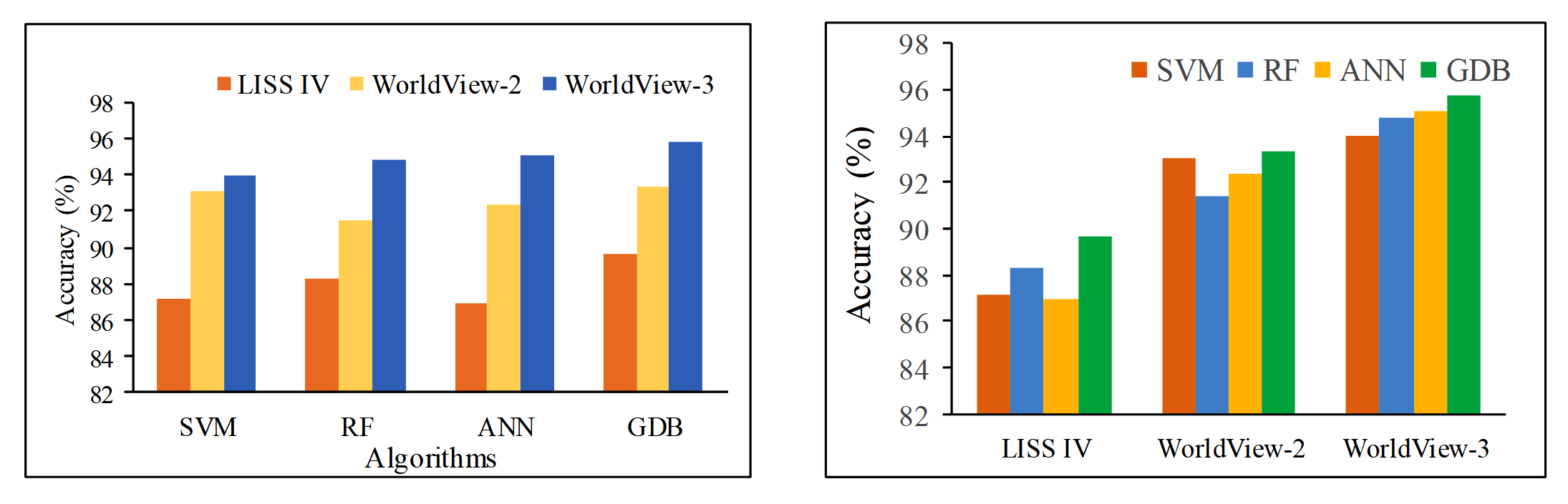
The targets of this study were: (a) to find the potential of the machine learning algorithms i.e. SVM, RF, ANN in building extraction from high-resolution satellite imagery and (b) to test and evaluate the ensemble learning technique in enhancing the performance of extraction of buildings. The complete statistical measures are shown in tables 2, 3 and 4 for various algorithms. Ensemble showed greater accuracy in three imageries. For the WorldView-2 imagery, SVM showed higher accuracy followed by ANN and RF. In WorldView-3, highest accuracy was showed by ANN followed by RF and SVM. This study showed that ANN performs significantly in uniform and linear building distribution on very high-resolution imagery. while RF showed good accuracy in the non-linear and heterogeneous distribution of urban buildings.

SVM worked very well in nonlinear building distributions as in WorldView-2 and optimal performance in other building distributions. It is observed that highest sensitivity is observed for RF for LISS-IV, while, lowest was shown by SVM. An equal degree of sensitivity is observed for both SVM and RF in WordView-2 imagery. The equal degree of sensitivity is observed for all three algorithms in case of WordView-3 imagery.

Gradient boosting algorithm showed improvement in accuracy of classification over single classifiers, it showed 1.58%, 0.2% higher accuracy and sensitivity, respectively than best performing algorithm in the LISS-IV imagery, 0.25% higher accuracy and 0.1% lower sensitivity than the best performing algorithm in WordView-2 imagery and 0.73%, 0.3% higher accuracy and sensitivity than best-performing algorithm in WordView-3 imagery.

After applying morphological operators and cleaning filters on LISS-IV imagery it was observed that it could not retain building occupying less than 10 pixels or area of less than 336.4 square meters due to a coarser resolution. While, for others morphological operators clean the salt and pepper noise, refining the footprints of the buildings. In very high resolution nearly every building was correctly classified, but some parts of the roads were misclassified as buildings pixels.

It showed that algorithms mathematical and statistical way of working has an impact on their classification pattern for a building distribution. The variation of accuracies of algorithms is due to variable building distributions and spatial resolutions of the imagery. As expected higher accuracy in all conditions is observed for the ensemble algorithm as it maps complex relationship from the outputs of the base algorithms, thereby corrects the misclassified pixels by the algorithms. Building detection rate by ensemble method for high-resolution imagery observed was 91.30% and 95.05%, while a building getting detected erroneously (Branching factor) is 10.01% and 4.01%. The decrease is seen due to the linearity of house construction with less spectral mixing. While, SVM showed nominal behavior but, works very well in some complex parts of the imagery where other algorithms show discrepancy, because even if it can’t find a linear decision boundary it can projects data points in multidimensional space to find a decision surface for this Radial basis function is used, thereby, separating the points. However, there are some disadvantages of support vector machine, those are large number of calculations due to large number of support vectors and during testing, its speed of classifying points becomes very slow and many critical parameters are to be set. SVM method of classification produced salt and pepper noise, which could be removed by morphological operators and cleaning filters. Use of ANN showed no improvement in accuracy if the number of hidden nodes is increased after a certain number, using fewer features or attributes as input produced low extraction results, and learning rate is a significant effect on neural networks, finding an optimal learning rate is important for accuracy. It showed higher overall accuracy for high-resolution imageries. Finding optimal parameters for neural networks requires an extensive combination of parameters. While RF can actually distinguish confusing urban objects increasing their probability of detection with stable classification accuracy without loss of information hence, works well both in low and high-resolution imagery.

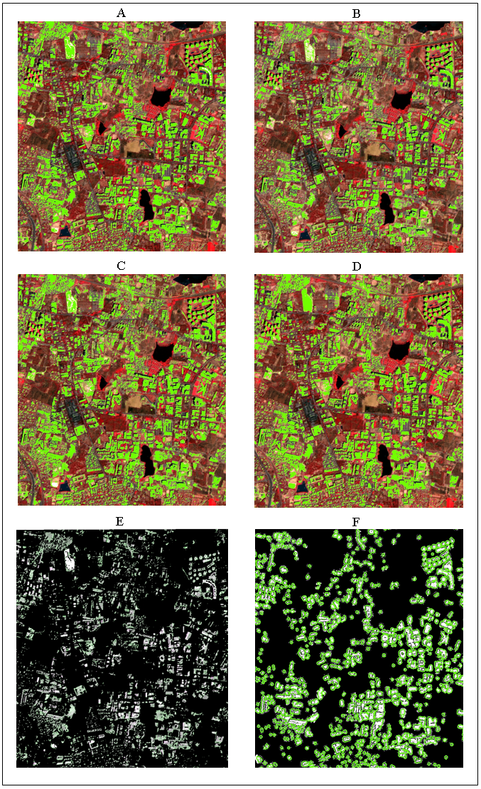
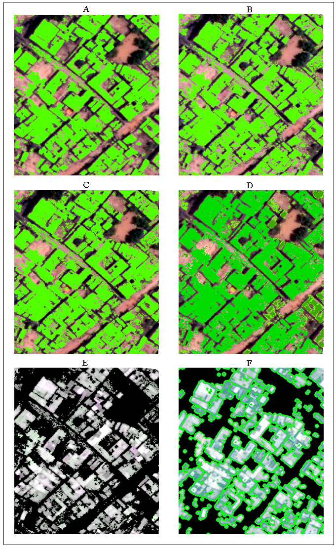
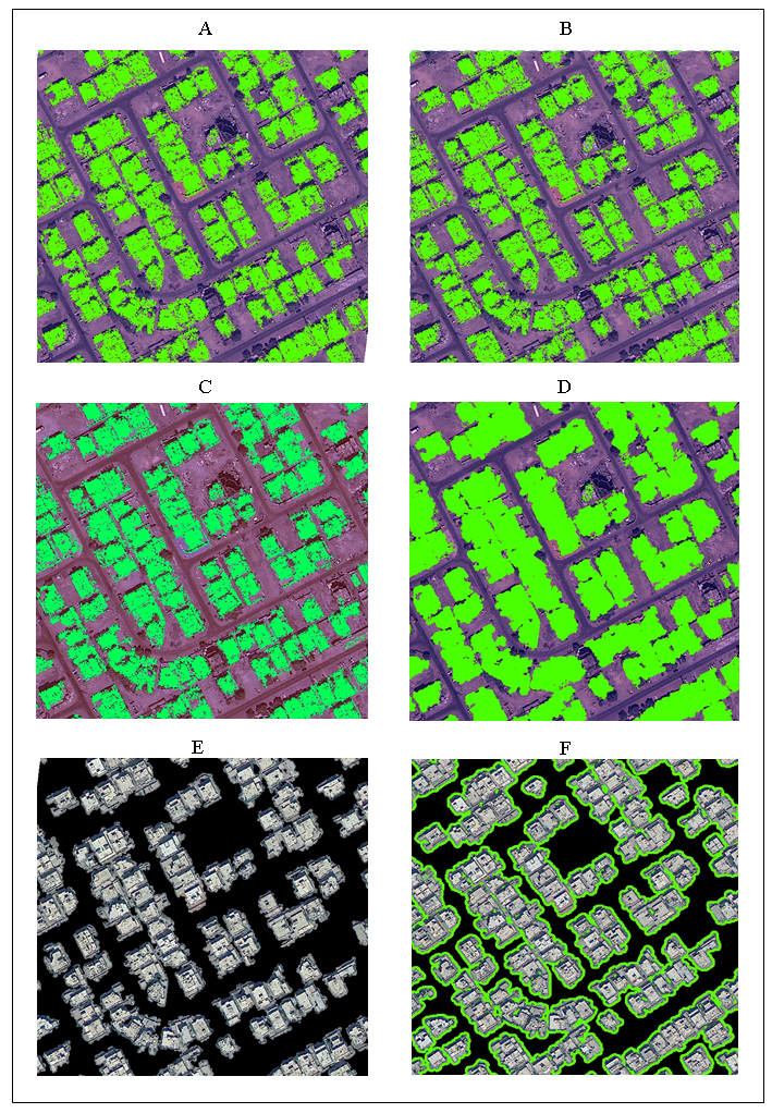
Building extraction results of different algorithms (figure 7- A, B, C, D) overlaid over imagery and final building extraction results for a subset of LISS-IV imagery (Figure 7). Final building extraction results for a subset of WorldView-2 imagery is as shown in figure 8.

Figure 7. Building extraction for a subset of LISS-IV imagery: (A) SVM, (B) RF (C), ANN, (D) GB, (E) building extraction before and (F) after applying morphology operators

Figure 8. Building extraction for a subset of WorldView-2 imagery (A) SVM, (B) RF, (C) ANN, (D) GB, (E) Building Extraction before and (F) after applying morphology operators

Figure 9. Building extraction for a subset of WorldView-3 imagery (A) SVM, (B) RF, (C) ANN, (D) GB, (E) building extraction before and (F) after applying morphology operators

Evaluation of detection rate in both images from Worldview 2 and Worldview 3 is shown in table 5. Comparable performance is tabulated graphically in figure 1.

Figure 10. Comparable performance of the algorithms on different satellite imageries with different building distribution patterns

6 . CONCLUSION

In this study, various types of machine learning algorithms and an ensemble learning technique were used for building extraction. These machine learning algorithms were successfully implemented for extraction of buildings with algorithms showing various amount of accuracy in different building distributions. Ensemble learning algorithm, which is the gradient boosting used for enhancing the classification accuracy, was successfully implemented for efficient building extraction from the high-resolution imagery. This is machine learning algorithm exploits various vegetation indices, PCA, spectral properties of the image which were fused into a single vector and where used for urban building extraction. It is observed that the overall performance and accuracy of the machine learning algorithms increased when the spatial resolution was increased with decreased misclassification rate. It is also observed that coarser resolution imagery such as in LISS-IV imagery building occupying less than 10 pixels or area less than 336.4 square meters were not captured with higher misclassification rate and also few barren lands where misclassified as buildings. However, most of the buildings were captured properly with edges being detected and shape being maintained. While in very high-resolution imagery algorithms worked very well with high building detection rate and higher accuracy. Based on this study, RF showed good performance in coarse resolution imagery, while Support Vector Machine and Artificial Neural Network showed optimal performance in all conditions and good in high-resolution imagery while the ensemble algorithm was considered best for efficient extraction of buildings from imagery. Specifically, the individual algorithms are repeatedly misclassifies the particular part. Hence, it’s observed that individual algorithms perform well in building extraction, while, ensemble learning could be used for increasing their accuracy of extraction.

Tables

Figures

Conflict of Interest

Acknowledgements

Abbreviations

References