Biomass stock was calculated by extrapolating the biomass stock measured from plot.
The linear relationship was observed as most of the trees in the study area were young with mean DBH of 20 ± 7.5 cm and mean height of 13. ± 6.2 m.
Site specific and species specific allometric equations are essential to accurately estimate biomass of the forest.
Fire risk modeling using multi-criteria analysis and integrating different layers used for Fire Risk Hazard Zonation.
Forest area near by the settlements, open area (Shrub land) and road are more vulnerable to forest fire.
The results and methodology used in this study can be useful for application of RS and geospatial technique for estimations of above ground biomass and Fire risk zonation.
Abstract
The drive for robust, accurate and cost-effective methods for biomass estimation over large areas is ever great with the launch of carbon crediting mechanisms in the developing countries such as UN-REDD [United Nations Programme on Reducing Emissions from Deforestation and Forest Degradation] and climate change mitigation program. Traditional ground based measurement requires abundant manpower, resources, cost and time. Remote sensing based technologies pertinently answer the need of time in enhancing the successful implementation of such programs. The region growing and valley following algorithm used to delineate individual tree crowns produced a segmentation accuracy of 59.35% and 54.83%, respectively. Both algorithms have similar approaches for delineation. Above ground biomass was calculated using allometric equation form and height, diameter measured from the field. Linear regression models were applied to derive the relation of biomass with crown projection area, field measured height with biomass. All models were significant at 95% confidence level and the lowest Root Mean Square Error (RMSE %) of 27.45 % (Shorea robusta) and 33.33% (others species). The total amount of biomass stocks was approximately 30620 Kg/ha-1. For forest fire hazard zonation an Analytic Hierarchy Process (AHP) method was used .The result show that 11% of the study area falls under very low fire risk zone, 55 % falls under low fire risk zone and 30 % falls under moderate fire potential zone while 4% of area falls under high forest fire risk zone. The map is also validated through major past fire incidents. The results show that the predicted fire zones are found to be in good agreement with past fire incidents, and hence, the map can be used for future forest resources management.
Keywords
Nepal , Forest Fire Risk Zonation , APH , Crown Projection Area , valley following , region growing , Individual tree crown
1 . INTRODUCTION
Reducing emissions from deforestation and forest degradation alongside with conservation and sustainable managing of forests in developing countries (REDD+) is emerging as a current tool to mitigate and adapt the impacts of climate change (Angelsen, 2008; FAO, 2016). As per the Intergovernmental Panel on Climate Change (IPCC) fifth assessment report, forest sector contributes 17.4% of greenhouse gases and most of this is contributed to forest deforestation and forest degradation. In this context the theory of “reducing of emissions from deforestation and forest degradation and the role of conservation, sustainable management of forests and enhancement of forest carbon stocks in developing countries” (REDD+), is decided at the Copenhagen Conference of the Parties (COP15) to the UNFCCC (Joseph et al., 2013). In this regard, a number of developing countries are resounding out pilot projects and readiness activities with monetary support from different finance schemes of developed countries. At present around 50 countries have started activities to be ready for REDD+ (Saito-Jensen et al., 2014). In 2010, at Cancun Mexico Measurement, Reporting and Verification (MRV) were considered as a critical element of climate change under climate change agreements for effective implementation of any REED+ mechanism. The monitoring and reporting of the present carbon resources can be achieved with many different approaches, official guidelines for REDD MRV are yet to be established (Gibbs et al., 2007). IPCC (2006) guidelines describe three tiers providing more reliable data so a higher financial return could return. These three tiers are characterized by data produced with process-based models allowing transparent and accurate reporting, providing reliable and valid information updated over time and site-specific.
In order to achieve tier 3 level information, there is the need to have a robust methodology that can be replicable over the years. Remote sensing techniques in combination with ground truth data can be used to build statistical models in order to fulfill Tier 2 and 3 requirements (Gibbs et al., 2007). Globally Nepal is considered as a leader in the community lead forest management (Pokharel, 2012) as in the 1990s Nepal’s Community Forestry Program (CFP) expanded momentum after the government prepared special rations for community forests in Section 5 of the Forest Act 1993 and Section 4 of Forest Regulation 1995 (Niraula et al., 2013). Nepal has been nominated as one of the four countries for promoting forest conservation by controlling deforestation and degradation as well as profiting off forest carbon stocks. The government of Nepal through its Ministry of Forest and Soil Conservation (MoFSC) have been preparing for REDD+ initiatives since 2008. Presently, Nepal is in the first phase; the readiness phase within which the Government of Nepal (GoN) develops a national REDD+ strategy, Intended National determined contribution (INDC) it had submitted to UNFCC on December 2015. Along with the destruction and degradation of forests, wildfires are emitting the huge amount of GHGs (IPCC, 2014). Field-based measurements give more precise biomass, but the collection of field measurements is time-consuming and labour-intensive, and it is impossible to census large geographic areas. Remotely sensed data benefit, such as repetitively of data collection, a synoptic view, a digital format that allows fast processing of large quantities of data and the high correlations between spectral bands and vegetation parameters make it the primary source for a large area above ground biomass (AGB) estimation in the remote area (Steininger, 2002; Chen et al., 2012; Shelly, 2012).
Therefore, both filed based measurement and remote sensing derived variables were used for aboveground biomass estimation. Analytic Hierarchy Process (AHP) with the different causative factors that are affecting forest fire like topographic parameters, vegetation parameters, and accessibility parameters were used for fire risk zonation.
2 . STUDY AREA
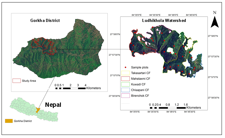
Ludhikhola watershed is located in the Gorkha district of the western development Region of Nepal (Figure 1). This watershed is having hill physiographic region with wide ranges of altitude ranging from 318 m to 1714 m from mean sea level. It has occupied 31 community forest user groups and managing about 1888 ha of forest area. Among 31 only 5 community forest was selected for this study.
Figure 1. Study area
3 . MATERIAL AND METHODS
The main material used for this research was the remote sensing data, GIS data layer, field data and software for the image and statistical analysis.
3.1 Very High-Resolution Geo-Eye Imagery
The ortho-rectified and geo-referenced Geo-Eye imagery with panchromatic (0.50m) and Geo-Eye multispectral (2m) images recorded 15th December 2012 were used for this study (Table 1). This multispectral image consists of four bands namely blue (450-510 nm), green (510-580 nm), red (655-690 nm) and near-infrared (NIR) (780-920).
Table 1. Data used
Image
Spatial Resolution
Spectral Bands
Geo Eye- 1
0.5 m
Panchromatic
GeoEye -1 Multispectral
2 m
4(Blue, Green, Red, NIR)
Date: December 2012
3.2 Reference Data and Processing
Topographic maps, Digital Elevation Model (DEM) 90M from SRTM digital elevation data, produced by NASA, MODIS fire point from 2010 to 2013, Gorkha geo-database which consist with different data layer namely vegetation types, watershed boundary, community forest boundary, road. For the preparation of base data layers, digitally scanned and extracted layers of the topographic sheets were acquired from National Geographic Information Infrastructure Project (NGIIP), Department of Survey (DoS), Nepal. The data layers correspond to topographic sheets of scale 1: 25,000/50,000 based on 1996 aerial photographs for western Nepal published in 1995 and onwards.
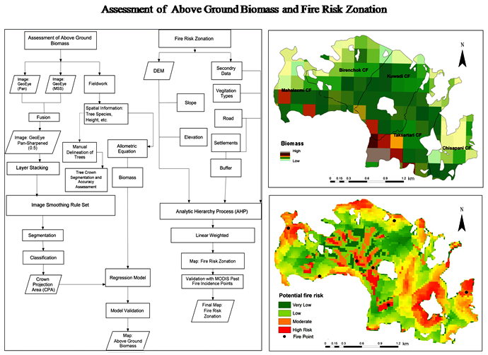
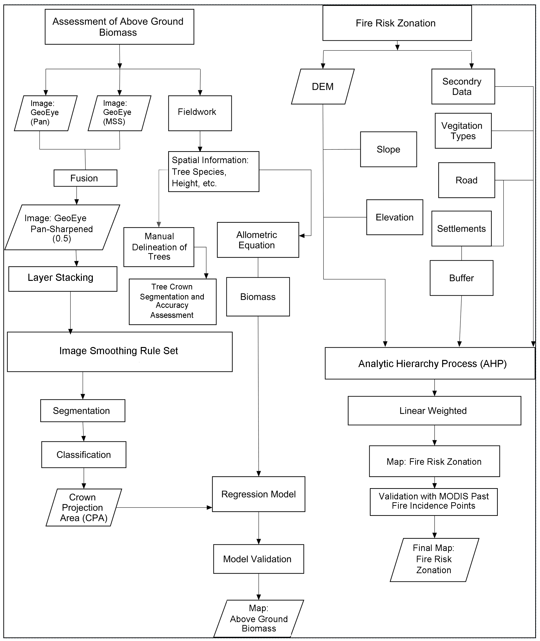
These datasets help to prepare the GIS maps to carry out forest resource assessments and field campaigns in the study area for forest biomass stock assessment and fire hazard mapping. Image analysis was done using ERDAS imagine and eCognition developer software for object-based image analysis. ArcGIS was used to carry out GIS operations and map formation. Microsoft office and other statistical packages were used for a write-up and statistical analysis. A diagram of the entire methodology applied in the study is shown in Figure 2.
Figure 2. Methodology
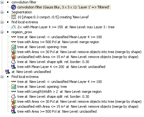
Figure 3. Rule Set in eCoginitation
3.3 Sampling Design
A sample is a set of data collected and/or selected from a statistical population by a defined procedure to obtain information about the population. To save resources, time and money sampling method are carried out rather than collecting census data from whole population. For carbon/biomass inventory, stratified random sampling generally yields more precise estimates for the other options (MacDicken, 1997). Therefore, for this study stratified random sampling was use to design the sampling process in the field. The strata were stratified based on 5 different community forests which are distributed in total of 379.153 ha. Total of 28 plots were identified for sampling in the field, 5 in each community forest and 3 additional plots were added in field because of some scatter distribution of forest area in those forest. The sampling plots were generated with the help of the secondary data and by using the sampling equation of (Husch, et al., 2003). Following equation was deployed to generate sample size:
\(n = {t^2 \times CV^2\over (E \%)}\) (1)
Where, n= number of sampling plots, t = t-test, CV = coefficient of variance, E= allowable error
3.4 Fieldwork
The fieldwork was carried out in order to measure the above-ground biomass and collect ground truth data. In the beginning of the fieldwork, an exploration visit was made to get an overall impression of the situation. Then, a meeting was held with the representatives of community forest user groups for further planning for data collection. During the fieldwork circular plots of 500m2 and radius of 12.62m each were collected. As per IPCC (2003) guideline then all the trees having the diameter at breast height equal or greater than 5 cm are considered as tree. The tree height was measured using Vertex IV and transponder and tree diameter at breast height (DBH) was measured using diameter tape. During the measurement, we considered and counted as two trees if forking was <1.3 meter of height from ground level (DBH) and single trees if forking was >1.3 m of height.
3.5 Detection of Crown projection Area and Delineation
To detect and delineate crown projection area (CPA) by applying region growing technique:
Loading image in eCoginitation Developer,
Loading and executing rule sets,
Image filter (Convolution filter),
Segmentation (Multi-resolution segmentation),
Find segments local Extrema Region grow,
Assign class and saving CPA as a shape file.
3.6 Manual Delineation of Tree Crowns
The delineation of the recognized tree crowns was done for assessing the segmentation accuracy and validating the model. For this purpose, both panchromatic and 5*5 filtered pan-sharpen image was used in such a way that tree crown can relatively easy to be recognized. Both images were visualized in ArcGIS at several scales for the better view of tree crown using appropriate band combinations. Pan-sharpened and panchromatic images were checked and unchecked alternatively during the crown delineation for a better result. Out of total 647 trees, about 40% trees measured from the field were delineated for accuracy assessment.
3.7 Accuracy Assessment of Tree Crown Delineation
Accuracy assessment of tree crown delineation is associated with alike of reference and automatically segmented objects (Zhan et al., 2005). Reference objects mean manually delineated polygons. There are several methods available for segmentation validation. However, two segmentation accuracy measures were applied i.e. 1:1 correspondence (Zhan et al., 2005) and Relative Area Measures developed by Clinton et al. (2010).
These schemes are applied when manually delineated and automatic segments are available. Clinton et al. (2010) reviewed several segmentation accuracy measures and modified Relative Area measures developed by Möller et al. (2007). Over-segmentation and under-segmentation defined by Clinton et al. (2010) are given as (equation 2 and 3):
\( Over \ segmentation= 1-{area (x_i \cap y_j) \over area (x_i )}\) (2)
\( Under \ segmentation= 1-{area (x_i \cap y_j) \over area (y_i )}\) (3)
where, \(x_i\) the reference is object and \(y_i\) is the corresponding segmented object.
The value of over-segmentation and under-segmentation lies within the range of 0 to 1 (Clinton et al., 2010). When the value for both over and under-segmentation is 0, then it is considered as perfect segmentation. It means that segments matched exactly with the reference objects. Using over segmentation and under-segmentation values, segmentation goodness (D) can be calculated. D (equation 4) is interpreted as the ‘closeness’ to an ideal segmentation result, in relation to a predefined reference object (Clinton et al. 2010). D value ranges from 0 to 1.
\(D= {Over \ segmenation^2+ Under \ segmenation^2 \over 2}\) (4)
1:1 correspondence was done by matching manually delineated tree crowns with automated segments. Corresponding was considered if manually delineated and automatic segments overlap by at least 50% (Zhan et al., 2005). The method proposed by Möller et al. (2007) was used for the accuracy assessment of tree crown segmentation. A higher percentage of 1:1 correspondence indicates higher accuracy.
4 . MAPPING AND MODELING OF BIOMASS STOCK
4.1 Calculation of Biomass Stock
In general, AGB is estimated from a volumetric and structural dimension of the trees for which DBH and height are considered as major parameters. In absence of species-specific biomass equation of the trees, species-specific volume equations developed by (Sharma and Pukkala, 1990) were used to estimate the AGB of forests.
Total stem volume of individual trees was calculated from field measured DBH and tree height using the relationship in the following form (equation 5) (Sharma and Pukkala, 1990).
ln(V) = a + b * ln(DBH) + c * ln(Ht) (5)
where, ln is natural logarithm to the base 2.71828, V is the total stem volume with bark in m3, to obtain the volume in cubic meters the prediction is to be divided by 1000, DBH is the diameter at breast height in cm, Ht is the tree height in m and a band c are model parameters.
The estimated parameter value of a, b and c for different species and wood density of the major tree species is given in Table 2.
Table 2. Model parameters and wood density of major trees
Species
a
b
c
Wood density (Kg/m3)
Shorearobusta
-2.4554
1.9026
0.8352
880
Others
-2.3993
1.7836
0.9546
720
The obtained volume was multiplied with dry wood density (specific gravity) of the species to get air dry weight of stem (Chaturvedi and Khanna, 1982) using the formula (equation 5). Species found in the study area other than mentioned above was categorized as miscellaneous in Terai and volume was calculated (equation 6) accordingly.
Stem biomass = Stem volume * Wood density (6)
Due to absence of established biomass relationship of different tree components of individual tree species of sample forest types, this study used the relationship developed by Sharma (2011) for a single species of similar forest types of Nepal which was later adopted by Shrestha and Singh (2008). The biomasses of branches and leaves (foliages) were estimated to be 42% and 8% of the stem biomass, respectively (Sharma, 2011) to calculate the total biomass (equation 7) of trees.
The regression model was used to analyse biomass. The multiple regression analysis is the most common tool for AGB estimation models (Lu, 2006). The relationship between the dependent variable (AGB) as obtained from the allometric equation and the two independent variables (tree height obtained from field and the plot level CPA from the segmented tree crowns were explored through log transformed regression models. Two most widely used methods for model validation are a coefficient of determination (R2) for the models developed and the root means square error (RMSE) (Lu, 2006). Co-efficient of determination (R2) shows the percentage of variation in one variable that is associated with other variables. The strength and the significance of the models were validated using the partitioned 30% validation dataset. The following equation (v) was used to calculate the RMSE.
where, XO = Observed biomass, Xp= Predicted biomass, n = number of observations
4.3 Variables of Fire Risk
The hierarchical structure for quantifying environmental risk has been intended the Analytical Hierarchy Method (Ramanathan, 2001; Gaikwad and Bhagat, 2017). The different predominant causative factors that affecting forest fire are topographic parameters, vegetation parameters and accessibility parameters (Bajracharya, 2002; Mohammadi, 2010). Elevation is an important physiographic factor that is related to wind behavior and hence affects fire proneness. Similarly, fire travels most rapidly up slope and least rapidly down slope. Likewise vegetation must be considered because some vegetation types are more flammable than theirs, thereby increasing the fire hazard. Road networks and settlement are other important variables.
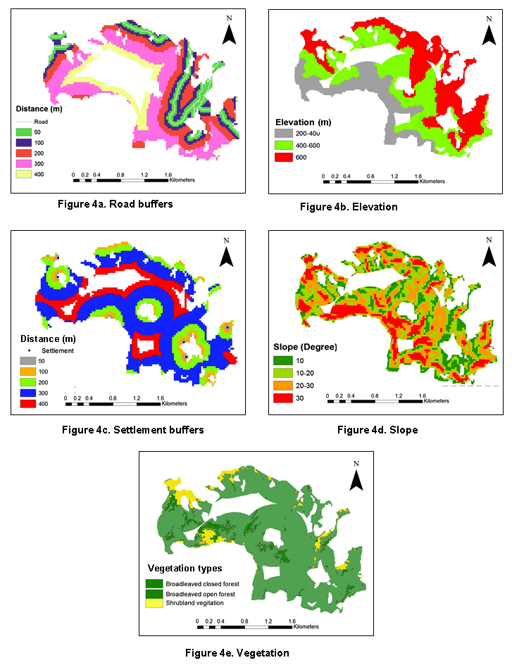
Previous studies in similar area showed that closeness to roads, settlements and agriculture lands increase the risk of fire. For this study also similar parameters were developed in GIS environment and classified accordingly as shown in figure 4. All values were used for Analytic Hierarchy Process (AHP).
Figure 4. Variables
5 . RESULT AND DISCUSSION
5.1 Pre-Processing of Images
The pan-sharpened, an image was pre-processed using 3 x 3 low pass filters which worked better for the region growing algorithm and 5 x 5 low pass filter image was used for valley following algorithm in eCognition. The processed filtered images are shown in the figure 5.
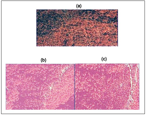
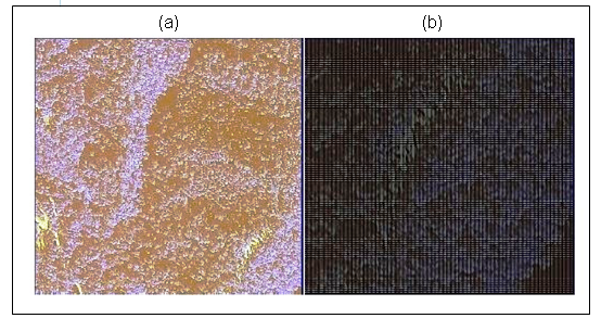
Figure 5. GeoEye image (a) IHS pan-sharpened image, (b) smoothed image using 3x3 low pass filter and (c) smoothed image using a 5x5 low pass filter (Images are at 1:700)
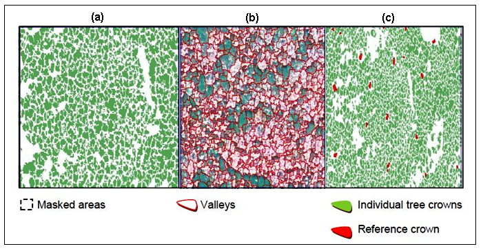
Figure 6. Valley following algorithm: (a) White area masked as non-vegetated area, (b) Valley following algorithm and (c) Individual tree crown overlaid with manually digitized trees.
5.2 Individual Tree Crown Delineation
5.2.1 Valley Following Algorithm
The segmentation in ITC suite follows mainly the three processes before delineating an individual tree crown. To delineate the individual tree crown the thresholds for upper limit (700-900) and lower limit (300) both the thresholds were used in NIR band.
5.2.1 Region Growing Algorithm
Pan-sharpened images were used as a distinctive layer for segmentation. 2 x 2 pixels chessboard segmentation algorithm was applied to the stacked layers of pan-sharpened MSS GeoEye image (0.5 m spatial resolution). The reason of the chessboard segmentation was for separation of the image into homogenous objects for individual tree crown delineation to build similar homogeneity conditions. Figure 7 shows a process of chessboard segmentation and pan-sharpened image.
Figure 7. (a) Panchromatic image and (b) Chessboard segmentation of the panchromatic image using tile size of two pixels
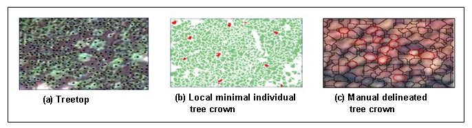
Further, the individual tree crown was delineated by locating the local maxima and minima of the treetops. Figure 8 (a) shows the identified treetop using local maxima, Treetops are the brightest point of the crown shown as a black cross in the image. The region growing algorithm is then applied to grow the treetops in an individual tree crown. Since it is an iterative process the region growing continues until it reaches the local minima as in shown in figure 8 (b) as a red mark. In figure 8 (b) the green color shows individual tree crowns obtained using region growing. The region growing algorithm is then applied to grow the treetops in an individual tree crown.
Figure 8. illustrates: (a) Black cross corresponds to treetop identified by the local maxima, (b) Fully delineated individual and (c) Manual delineated tree crowns (red color) superimposed on the automatic segments (black color)
6 . ACCURACY ASSESSMENT OF VALLEY FOLLOWING AND REGION GROWING ALGORITHM
6.1 Assessment using Goodness Measure Approach
Inter-sector tool was used for the accurate measurement of two algorithms namely region growing and valley following. To calculate D value this gives an overall result of over-segmentation and under segmentation. Higher accuracy will be for D index closer to 0. The segmentation accuracy explains that using valley following algorithm the D value = 0.43 so this explains it delineated only 57 % of the crown correctly whereas using region growing algorithm the D value =0.29 which explains 71 % of the trees were correctly delineated and using the same reference crown for accuracy assessment (Table 3).
1to1 matching was done to check the positive identification of the trees. The reference crown and segmented crown were overlapped and only those trees which overlapped 50% or more were considered as correctly delineated. Out of 155 identified trees valley following were able to detect 85 trees only (Table 4) whereas region growing were able to detect 92 trees correctly. Remaining trees were missed by an algorithm. 1 to 1 matching of individual tree crown is shown in table 2.
Table 2. Model parameters and wood density of major trees
Species
a
b
c
Wood density (Kg/m3)
Shorearobusta
-2.4554
1.9026
0.8352
880
Others
-2.3993
1.7836
0.9546
720
Table 3. Segmentation accuracy of valley following and region growing algorithms
Segmentation
Valley following
D value
0.43
Over segmentation
0.38
Under segmentation
0.42
Overall segmentation accuracy
57%
Table 4. 1 to 1 matching of individual tree crown
Valley following
Region growing
Positive identification of trees
85
92
Detection rate (%)
54.83%
59.35%
Total reference trees are 155.
6.2 Biomass Stock
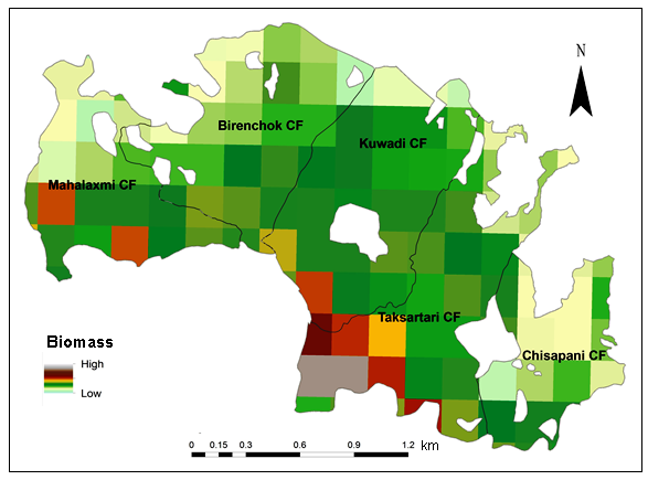
Above ground biomass stock was accessed from field measured diameter at breast height (DBH) and height by using the species-specific allometric equation for the study area. Biomass stock of individual trees was calculated species-wise then total carbon of trees measured in the sampling plots were calculated and averaged (i.e. per plot) for each community forest. Biomass stock per ha was calculated by extrapolating the biomass stock from plot (500 m2) to ha. Total biomass in different five community forests: Taksartari, Kuwadi, Birenchok, Mahalaxmi and Chisapani Community forest are shown in table 5.
Table 5. Above ground biomass in different community forest
Name of community forest
No. of plots
Area of CF (ha)
Biomass (tons/ha)
Birenchok
5
84
193.25
Chisapani
4
50
163.71
Kuwadi
7
92
212.37
Mahalaxmi
5
64
201.41
Takasartari
7
89
219.45
Figure 9. Distribution of biomass
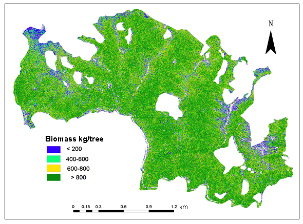
Figure 10. Biomass (per tree)
6.3 Regression Analysis
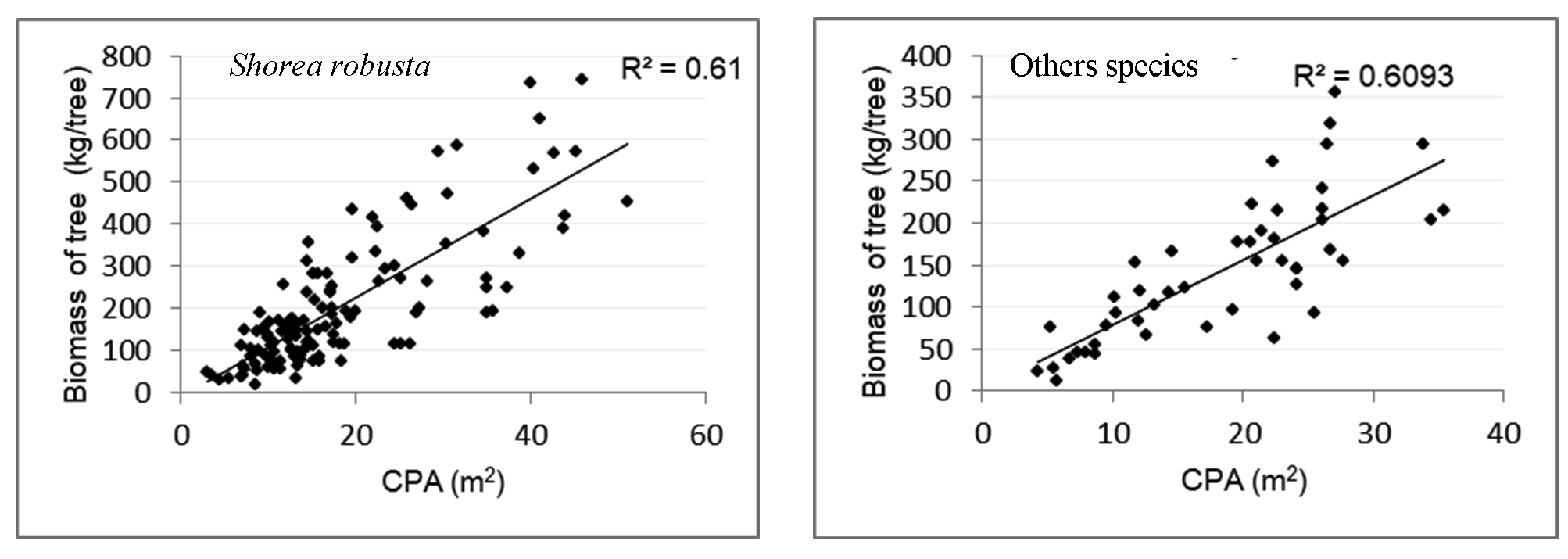
6.3.1 Relationship between CPA and AGB
Linear regression models were developed to derive the relationship between CPA and AGB for both Shorea robusta and other species. Total of 155 measurements were used for model development in case of Shorea robusta whereas a total of 80 measurements were used in case of the other species. The coefficient of determination (R2) for Shorea robusta and other species were 0.61 and 0.693, respectively. The regression analysis showed an acceptable correlation between CPA and AGB for both the classes with the correlation coefficient varying from 79% (Shorea robusta) to 78% (others). The models developed for biomass stock estimation of Shorea robusta and other species are.
One Way Analysis of Variance (ANOVA) test at 95% confidence level showed the significant relationship between CPA and AGB.
Figure 11. Relationships between CPA and AGB
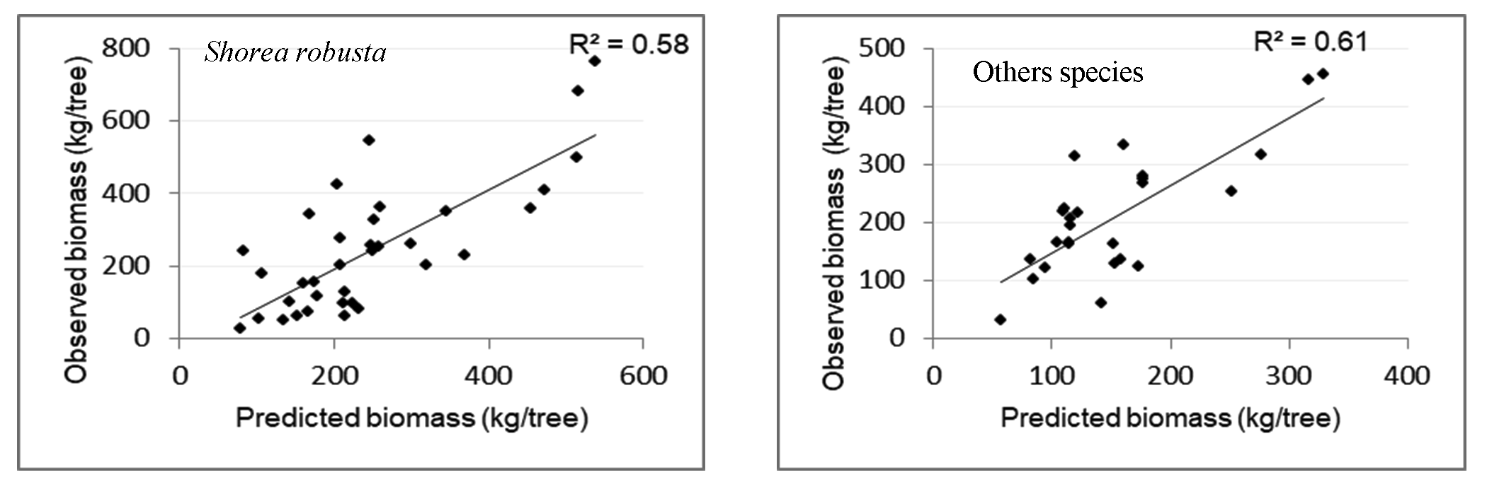
6.3.2 Model Validation
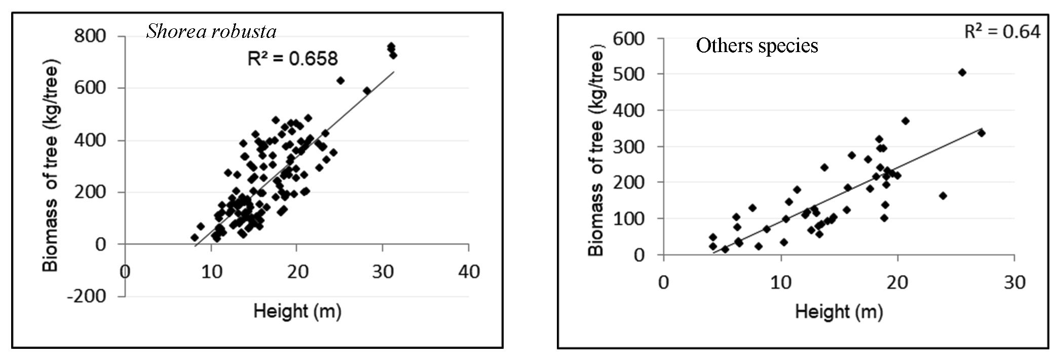
The developed model was validated against the field observed datasets (n=40, Shorea robusta; n=20, others). The results of the modeling corresponded well with the observed values commonly all models were explaining the relationship of biomass with CPA. Comparing all models, multiple linear regression models had the lowest RMSE % i.e. 27.61% and 33.33% for both Shorea robusta and other species, respectively. This means there is 27.61% average error in the prediction of biomass for Shorea robusta and 33.33% average error in the prediction of biomass for other species. The relationship between CPA and biomass for both classes of trees resulted in higher RMSE % i.e. 47.1% for Shorea robusta and 41.5% for other species. RMSE% of the model developed for height and carbon were 40.3% and 35.3% for Shorea robusta and other species, respectively. This means multiple regression models improve the accuracy of biomass estimation than other models.
Figure 12. Relationship between height and biomass
Figure 13. Relationship predicated and observed biomass
7 . AHP ANALYSIS FOR FIRE HAZARD ZONATION
As the AHP, introduced by Thomas Saaty (Habibi, K et al., 2008) is a mathematical method which analyses complex decision problems under multiple criteria and helps the decision makers to set priorities and make the best decision. Based on this technique fire hazard zonation was done. Evaluation of criteria is made using a scale from 1 to 9 if the factors have a direct relationship and a scale from 1/2 to 1/9 if the factors have an inverse relationship as shown in table (Table 7). Elements of the matrix in each level are compared in pairs with respect to their importance to the element in the next higher level.
Table 6. Sample of comparison of each classes of parameter Fire Hazard Zonation
Question 1
With respect to Fire Hazard Zonation mapping
Given that the distance from the settlements is <50 m which criteria is important?
Classes
50–100 m
100–200 m
200–500m
>500 m
Weight values
Question 2
With respect to Fire Hazard Zonation mapping
Given that the distance from the settlements is 50 m-100 m which criteria is important?
Classes
<50 m
100–200 m
200–500m
>500 m
Weight values
Question 3
With respect to Fire Hazard Zonation mapping
Given that the distance from the settlements is 100 m-200 m which criteria is important?
Classes
<50 m
100–200 m
200–500m
>500 m
Weight values
Question 4
With respect to Fire Hazard Zonation mapping
Given that the distance from the settlements is 200 m-500 m which criteria is important?
Classes
<50 m
100–200 m
200–500m
>500 m
Weight values
Question 5
With respect to Fire Hazard Zonation mapping
Given that the distance from the settlements is 500m which criteria is important?
Classes
<50 m
100–200 m
200–500m
>500 m
Weight values
Table 7. Pair-wise comparison matrix and normalized principal eigenvector for the classes within each causative factor of fire potential
Causative factors and classes within each factor
[1]
[2]
[3]
[4]
[5]
[6]
[7]
[8]
[9]
Normalized principal
eigen vector
Distance from settlements
[1] <50 m
1
2
4
6
9
0.456
[2] 100 m
1/2
1
2
3
6
0.347
[3] 200 m
1/4
1/2
1
5
7
0.105
[4] 300 m
1/6
1/3
1/5
1
2
0.073
[5] 400 m
1/9
1/6
1/7
1/2
1
0.019
Vegetation types
[1] Shrub land veg.
1
5
7
0.687
[2] Closed forest
1/5
1
5
0.234
[3] Open forest
1/7
1/5
1
0.079
Distance from road
[1] <50 m
1
2
4
7
9
0.423
[2] 100 m
1/2
1
2
3
9
0.255
[3] 200 m
1/4
1/2
1
5
7
0.190
[4] 300m
1/7
1/3
1/5
1
2
0.080
[5] 400 m
1/9
1/9
1/7
1/2
1
0.052
Slope in degree
[1] <10
1
1/2
1/3
1/4
0.26
[2] 10- 20
2
1
1/2
1/3
0.25
[3] 20-30
3
2
1
1
0.26
[4] >30
4
3
2
1
0.43
Elevation
[1] 200-400 m
1
1/2
1/3
0.104
[2] 400–600 m
2
1/3
1/3
0.399
[3] >600
3
2
1
0.497
In order to generate fire potential hazard map, the linear weighted combination is used for different causative factor as shown in Table 8.
Table 8. Number of order of matrix n, largest eigen value λ max of the preference matrix, consistency index (CI), random consistency index (RI), and consistency ratio (CR), for the fire potential causative factors
Causative Factors
n
λ max
CI
RI
CR
Distance from settlements
5
5.01
0.002
1.12
0.003
Distance from road
5
5.25
0.06
1.12
0.056
Land cover
3
3.06
0.02
0.58
0.025
Slope
4
4.29
0.07
0.90
0.081
Elevation
3
5.02
0.005
1.12
0.005
Fire Hazard Zonation = Weight map of (distance from Settlements + forest cover + distance from road + Slope + elevation) (11)
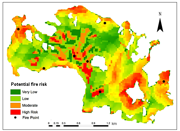
Settlement, accessibility, and forest types had played an important role in Fire Risk Zonation. The other variables elevation and slope have a comparatively less impacting estimation of fire risk zonation. The final forest fire risk model was validated with past fire incidences data that was collected from MODIS fire alert system.
Figure 14. Potential Fire Risk Zones
Table 9. Fire risk area
Fire Risk
Area
%
ha
Very Low
11
41.71
Low
55
208.54
Moderate
30
113.75
High
4
15.17
8 . CONCLUSION
Biomass is commonly estimated by applying conversion factors (biomass expansion factors) to tree volume (either derived from field plot measures or forest inventory data. The combination of remote sensing and ground-based inventory was applied to account forest aboveground biomass estimation in a study area. About 11607 tons of biomass was calculated from 28 plots which were located randomly throughout the study area with an average 30620 Kg biomass ha-1.Fire risk modeling using multi-criteria analysis and integrating different layers were used for developing fire risk hazard zonation map. Fire hazard is directly proportional to the distance from road, settlement and is more susceptible to fire risk than other parts of forest area.
9 . UNCERTAINTY
There were mainly four major operations in this study and in each operation error could be introduced. The segmentation accuracy showed errors. Commission and omission errors were observed due to overlapping trees and branches of big trees which can reach far in different directions and grow into irregular shape. The next operation was classification of tree species. When classification is not correct, accurate estimation of biomass is not possible. Error in classification may lead to selection of wrong wood specific gravity for a tree. Error in classification could be due to spectral characteristic of vegetation, shadows, distortion of the image and misidentification of tree. Selection of appropriate model is required. Data used for the model should be good representative of population (trees) in the study area. Otherwise, this might affect the model. Beside these, errors from allometric equation would affect the model. For fire risk hazard zonation, the main demerit of AHP method is that it has a subjective nature of the modeling process which may differ from one to another. Hence, methodology cannot guarantee the decisions as definitely true.
Tables
Figures
Conflict of Interest
The author declares no conflict of interest.
Acknowledgements
Author would like to express sincere gratitude to editors and, ICIMOD, Dr. Shahnawaz, Dr. Ram Asheshwar Mandal, Dr. Ambika Gautam, Chungla Sherpa for their valuable feedback, guidance and regular support.
Abbreviations
AGB: Above Ground Biomass; AHP: Analytic Hierarchy Process; CFP: Community Forestry Program; CI: Consistency Index; COP: Conference of Parties; CPA: Crown Projection Area; CV: Coefficient of Variance; DBH: Diameter at Breast Height; DEM: Digital Elevation Model; GIS: Geographical Information System; Ha: Hectare; INDC: Intended National Determined Contribution; IPCC: Intergovernmental Panel on Climate Change; MRV: Measurement Reporting and Verification; NIR: Near Infrared; REDD: Reducing Emissions from Deforestation and Forest Degradation; RI: Random Consistency Index; RMSE: Root Mean Square Error; UNFCC: United Nations Framework Convention on Climate Change.
Gaikwad, R. and Bhagat, V., 2017. Multi-Criteria Watershed Prioritization of Kas Basin in Maharashtra India: AHP and Influence Approaches. Hydrospatial Analysis, 1(1), 41-61.
MacDicken, K., G., 1997. A guide to monitoring carbon storage in forestry and agroforestry projects. USA, Winrock International Institute for Agricultural Development.
19.
Mahdavi, A., Shamsi, S. R. F. and Nazari, R., 2012. Forests and rangelands’ wildfire risk zoning using GIS and AHP techniques. Casptechniques.Asp. J. Environ. Sci. 10, 43-52.
20.
Mohammadi, F., Shabanian, N., Pourhashemi, M. and Fatehi, P., 2010. Risk zone mapping of forest fire using GIS and AHP in a part of Paveh forests. Iranian J. of Forest and Poplar Res., 18 (4), 569-586 (In Persian).
Sharma, E. R., and Pukkala, T., 1990. Volume Equations and Biomass Prediction of Forest Trees of Nepal. Kathmandu, Nepal: Forest Survey and Statistics Divison, MOFSC
Sharma, S. P., 2006. Participatory forest fire management: an approach. International Forest Fire News, 34:35-45.
29.
Shelly, J. R., 2012. Woody biomass: what is it- what do we do with it? Woody biomass factsheet-WB1. Washington D.C, US.
30.
Shrestha, B. M. and Singh, B. R., 2008. Soil and vegetation carbon pools in a mountainous watershed of Nepal. Nutrient Cycling in Agroecosystems, 81(2), 179-191.