3 . METHODOLOGY
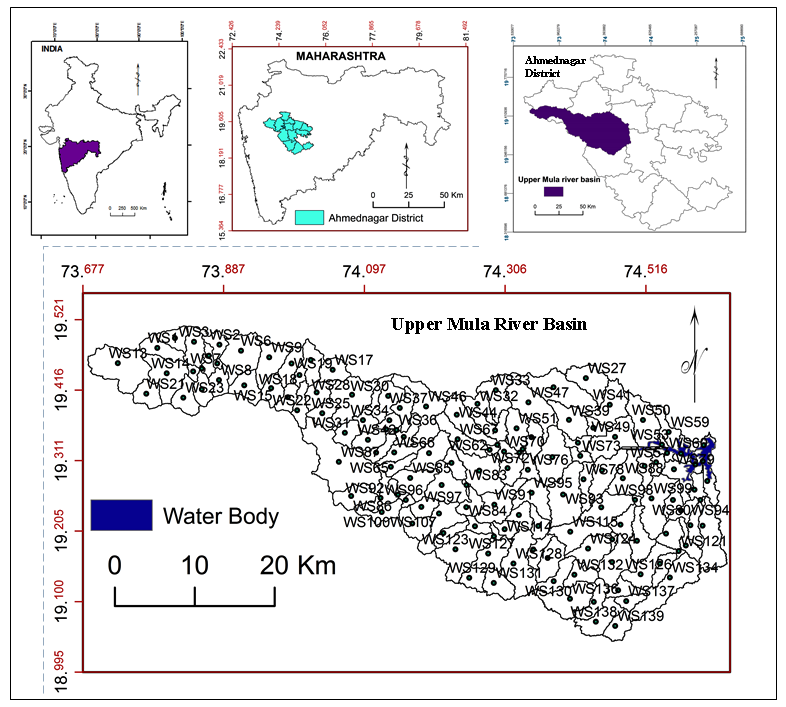
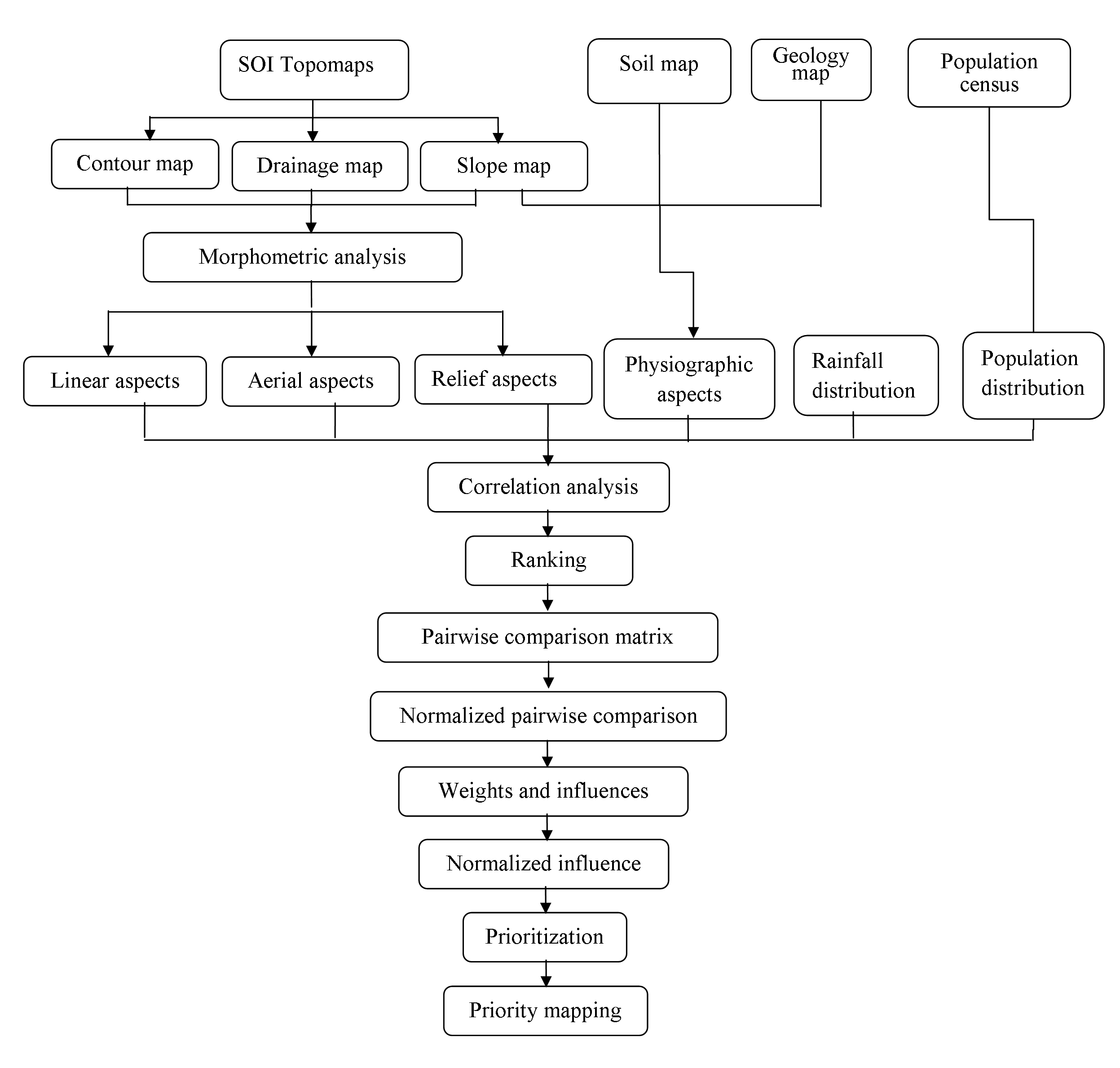
Multi-criteria analysis based on AHP and influence techniques was used for prioritization of sub-watersheds in Mula River basin, medium watershed located in Western Maharashtra. The prioritization was performed through eight steps: 1) delineation of sub-watersheds with help of DEM, 2) selection, measurements and analysis of criterion, 3) ranking of criterion, 4) pairwise comparison, 5) normalization on pairwise comparison matrix, 6) calculations of weights, 7) sub-watershed wise normalization of calculated influences, and 8) prioritization of sub-watersheds.
3.1 Data
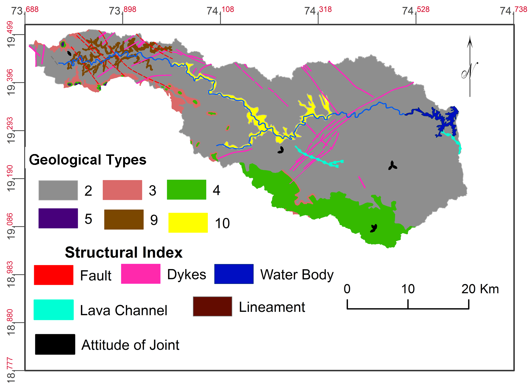
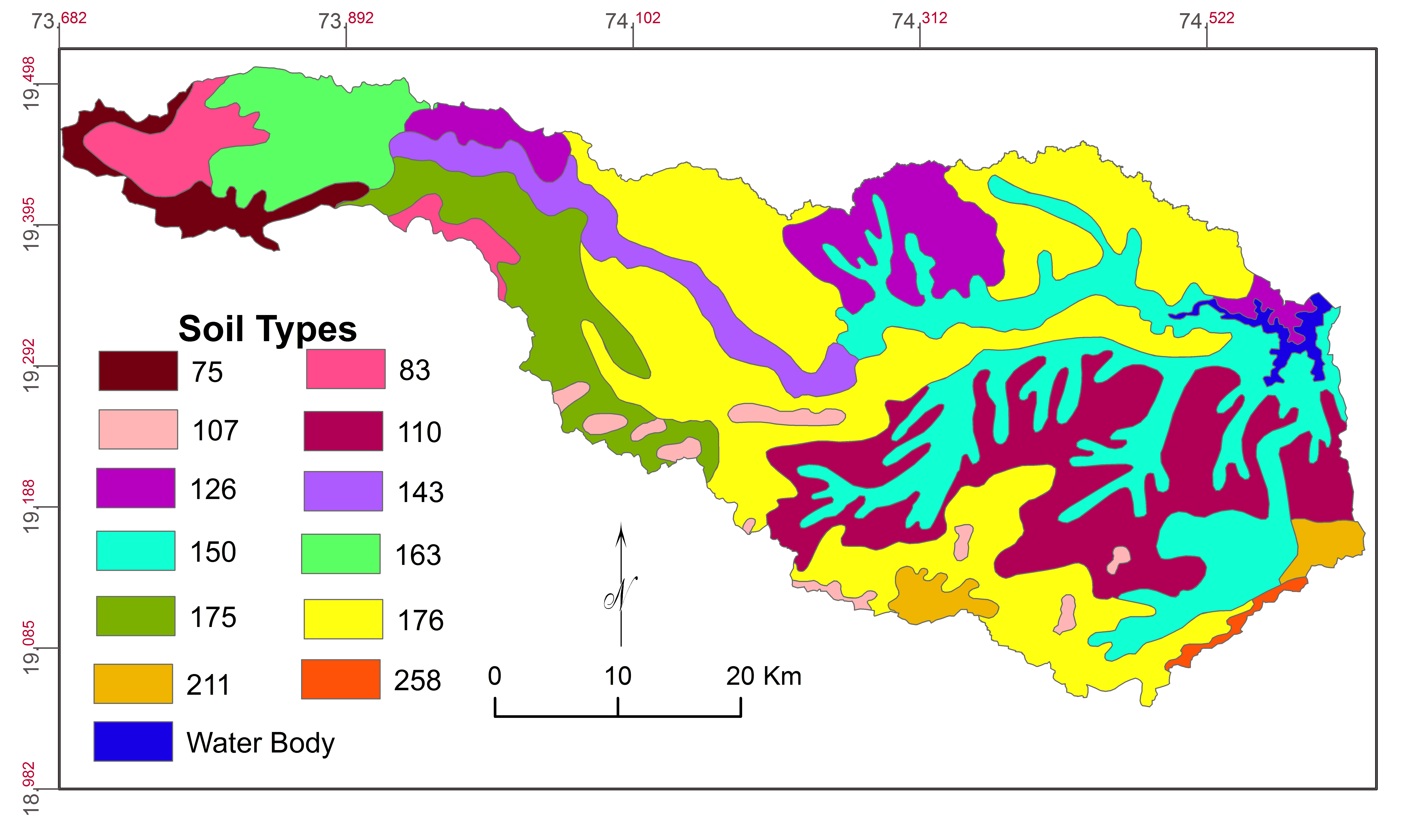
Information about geology, morphometric parameters, soil characteristics, rainfall and population density was used for multi-criteria and AHP analysis for prioritization of medium watershed. Geology is mapped (Figure 2) based on map procured from NIGS [National Institute of Geological Survey, Nagpur (India)]. Morphometric parameters: areal, linear and relief were calculated (Table 2) and mapped based on topographic maps (47E/10, 47E/11, 47E/14, 47E/15, 47I/2, 47I/3, 47I/4, 47I/6, 47I/7, 47I/8, 47I/10, 47I/11 and 47I/12) procured survey of India. Watershed boundaries were delineated using ASTER DEM data and soil map (Figure 3) prepared using map procured from NBSS and LUP [National Bureau of Soil Survey and Land Use Planning], India. Rainfall map (Figure 26) was prepared using the data recorded at raingauge stations (1992-2013) located from the study area and based on World climate data (mean rainfall from 1970 to 2000). Population data is taken from census report, 2011.
Table 1. Soil groups
|
Soil Code*
|
Soil characteristic
|
Area
|
|
Km2
|
%
|
|
75
|
Loamy soils: on moderate steep slopes (north) of Sahyadri Ghat; dissected escarpments with severe erosion; very shallow, extremely well drained with moderate erosion.
|
59.55
|
1.75
|
|
83
|
Clayey soil: shallow and well drained; on highly dissected ranges on north Sahyadri Ghat with moderate erosion.
|
59.55
|
1.75
|
|
107
|
Calcareous soils: on gently sloping peaks/spurs with moderate erosion; slightly deep; shallow well drained with moderate erosion.
|
83.95
|
2.47
|
|
110
|
Loamy and calcareous soils: on gently sloping undulating land with severe erosion; very shallow and highly drained.
|
37.92
|
1.12
|
|
126
|
Excessively drained loamy and well drained fine calcareous soils: slightly deep; on gently sloping land with severe erosion and slightly deep well drained fine calcareous soils with moderate erosion.
|
368.87
|
10.85
|
|
143
|
Shallow and well drained loamy and calcareous soils: on very gently sloping plains with moderate erosion.
|
166.09
|
4.89
|
|
150
|
Deep and well drained loamy and calcareous soils: on very gently sloping land with slight and moderate erosion.
|
100.75
|
2.96
|
|
163
|
Very shallow excessively drained loamy soils: on moderately sloping land, mesas and buttes with severe erosion.
|
422.85
|
12.44
|
|
175
|
Very shallow and excessively drained loamy and calcareous soils: on gently sloping with mesas and buttes with severe erosion; very shallow, excessively drained, loamy soil with very severe erosion and moderate stoniness.
|
152.59
|
4.49
|
|
176
|
Slightly deep, well drained and fine calcareous soils: on very gently sloping land with mesas and buttes; slight deep, well drained and fine with moderate erosion.
|
159.45
|
4.69
|
|
211
|
Slightly deep, well drained, fine, moderately calcareous soils: on very gently sloping land, slightly deep, well drained, fine soil with moderate erosion.
|
1717.48
|
50.52
|
|
216
|
Shallow, well drained, clayey moderately calcareous soils: on gently sloping land, moderate stoniness, slightly deep, well drained, fine and salinity moderately calcareous soils with moderate erosion.
|
53.1
|
1.56
|
|
258
|
Fine calcareous soils: deep, fine moderately well drained soil on gently sloping land with moderate erosion; on plains and valleys with moderate erosion.
|
10.04
|
0.30
|
3.2 Criterion
Spatial variations in geology, morphometric parameters, soils, rainfall and population were used for multi-criteria analysis using AHP and influence technique (Figure 4).
3.2.1 Geology
Watershed characteristics define due to nature of geology including subsurface materials and structure (Flint et al., 2013; Aouragh and Essahlaoui, 2014). Rate of infiltration, run-off, level of groundwater and hydraulic conductivity of surface are dependent on geology of the region (Engelhardt et al., 2011; Olden et al., 2012; Dhanalakshmi and Shanmugapriyan, 2015). The study area shows compound pahoehoe flows (12 to 15m) and som Aa flows, megacryast compound pahoehoe basaltic flows (50 to 60m), 5 Aa and 1 compound pahoehoe basaltic flows (up to 150m) and alluvium type geology (Figure 2). The hydrogeological properties of rocks and soils govern the occurrence, movement and storage of groundwater. Alluvial deposits are unconsolidated in nature and therefore act as good aquifers. Alluvium type of geology is more suitable for groundwater recharge and movements. However, literature reveals considerable variation in the hydrogeological properties of alluvium (Rao and Thangarajan, 1999; Raza et al., 2003; Watts, 2005; Kim et al., 2005). Further, Aa shows groundwater only in upper weathered, fractured and vesicular layers. Aa flows in the region can be classified as simple and compound types. The simple flows show thin blocky vesicular upper part and lower part is compact and fine-grained (Subbarao and Hooper, 1988; Ray et al., 2006; Mahoney et al., 2000; Melluso et al., 1995; Powar, 1987; Cox and Hawkesworth, 1985; Beane et al., 1986; Bodas et al., 1988; Khadri et al., 1988). Compact flows often show columnar jointing with weathered and fractured upper layers. Therefore, this type is considered as key criteria in this analysis.
3.2.2 Morphometric Parameters
Morphometric parameters like linear, areal and relief were processes in GIS environment (Gabale and Pawar, 2015) for multi-criteria analysis. We have used these morphometric parameters for prioritization of sub-watersheds successfully (Gaikwad and Bhagat, 2017).
3.2.2.1 Linear Aspects
The scholars like Khare et al. (2014), Rao et al. (2014), Aouragh and Essahlaoui, (2014), Farhan and Anaba, (2016) were used Linear morphometric parameters including stream orders (\(U\)), stream length ( \(L_u\) ), mean stream length \(L_{sm}\) ) (Wilson et al., 2012), stream length ratio ( \(R_{L}\) ), bifurcation ratio (\(R_b\) ) show relationship with erodibility of land surface. Therefore, many scholars have used these parameters as criterion for prioritization watersheds (Table 2).
Table 2. Formulae used for computation of morphometric parameters
|
Aspects
|
Parameters
|
Equation
|
Description
|
Author
|
|
Linear
|
Stream order (\(U\))
|
Hierarchical rank
|
The first step of drainage basin analysis.
|
Iqbal and Sajjad (2014); Raja and Karibasappa (2016);
|
|
Mean stream length( \(L_{sm}\) )
|
\(L_{sm}=L_u/N_u\)
|
\(L_u\)= stream length of order ‘\(U\)'
\(N_u\)= number of stream segments
|
Rekha et al. (2011); Zende et al. (2013); Farhan and Al-Shaikh (2017)
|
|
Bifurcation ratio ( \(R_b\))
|
\(R_b = (N_u)/(N_u+1) \)
|
\(R_b\) = bifurcation ratio
\(N_u\) = number of stream segments
|
Kulkarni (2015); Chitra et al. (2011); Romshoo et al. (2012); Jagadeesh et al., (2014); Aravinda and Balakrishna (2013); Schumn (1956); Kedareswarudu, et al. (2013), Iqbal and Sajjad (2014)
|
|
Stream length ( \(L_u\))
|
\(L_u =\displaystyle\sum_{i=1}^{N} U\)
|
\(L_u\) = mean length of channel
\(U\) = stream-channel segment of order
|
Horton (1945); Ali et al., (2014); Nongkynrih and Husain (2011); Kulkarni, (2015)
|
|
Aerial
|
Basin area ( \(A\))
|
\(A=a \times n \times10^{-6}\)
|
\(a\) : cell area(m2)
\(n\) : number of watershed cells
|
Romshoo et al. (2012); Thakur (2013)
|
|
Basin length (\(L_b\))
|
|
\(L_b\) = farthest distance from watershed ridge to outlet
|
Thakur (2013)
|
|
Basin perimeter (\(P\))
|
\(P=d \times np \times10^{-3}\)
|
\(d\) :cellsize(m)
\(np\) : number of watershed edge cells
|
Nagal et al. (2014); Thakur (2013)
|
|
Shape factor ( \(B_s\) )
|
\(B_s=L_b^2/A^h\)
|
\(B_s\)=shape factor,
\(A\)= area of the basin (km2), \(L_b^2\) = Square of the basin length
|
Patel et al. (2013); Kulkarni, (2015)
|
|
Drainage density ( \(D_d\))
|
\(D_d =\displaystyle\sum_{}^{} L_u/A\)
|
\(D_d\) = drainage density
\(L_u\) = total stream length
\(A\) = basin area
|
Kulkarni, (2015); Nongkynrih and Husain (2011); Nagal et al. (2014); Aravinda and Balakrishna (2013); Shing and Shing (2011)
|
|
Stream frequency ( \(F_s\))
|
\(F_s =\displaystyle\sum_{}^{} N_u/A\)
|
\(F_s\) = stream frequency
\(N_u\) = number of stream segments
\(A\) = basin area
|
Kulkarni, (2015); Nongkynrih and Husain (2011); Nagal et al. (2014); Aravinda and Balakrishna (2013); Shing and Shing (2011)
|
|
Form factor ( \(R_f\)
|
\(R_f=A/(L_b+1)^2\)
or
\(R_f=A/L_a^2\)
|
\(R_f\) = form factor
\(A\) = basin area
\(L_b\) = farthest distance from watershed ridge to outlet
or
\(A\) = area of the basin and
\(L_a\) = axial length of the basin.
|
Rao and Alia (2013); Ali et al. (2014); Kedareswarudu et al., (2013); Zende et al. (2013); Nagal et al. (2014); Iqbal and Sajjad (2014)
|
|
Circularity ratio ( \(R_c\))
|
\(R_c=4\pi (A/P^2)\)
|
\(R_c\) = circularity ratio
\(A\) = basin area
\(P\)= basin perimeter (km)
|
Rao and Alia (2013); Iqbal and Sajjad (2014); Ali et al. (2014);
|
|
Elongation ratio ( \(R_e\))
|
\(R_e = \frac {2}{\pi} \sqrt{\frac {A}{(L_b)^2}} \)
or
\(R_e = 2 \sqrt{\frac {A}{\pi}/L_u} \)
|
\(R_e\) = elongation ratio
\( \pi\) = 3.14
\(A\) = basin area or
\(L_u\) Total stream length.
|
Aravinda and Balakrishna (2013); Schumn (1956); Kedareswarudu et al., (2013); Thakur (2013)
|
|
Compactness coefficient ( \(C_C\))
|
\(C_c=0.2821 {\frac {P}{A}}0.5\)
|
\(C_C\) = compactness coefficient
\(A\) = area of the basin (km²)
\(P\) = basin perimeter (km)
|
Iqbal and Sajjad (2014)
|
|
Drainage texture ( \(D_t\))
|
\(D_t=N_u/P\)
|
\(N_u\) = total no. of streams of all orders
\(P\) = basin perimeter, km
|
Iqbal and Sajjad (2014); Zende et al. (2013)
|
|
Texture ratio (\(T\))
|
\(T=D_d \times F_s\)
|
\(D_d\) drainage density
\(F_s\) stream frequency
|
Nagal et al. (2014); Kedareswarudu et al., (2013)
|
|
Drainage intensity \(D_i\)
|
\(D_i=F_s/D_d\)
|
\(D_i\) = drainage Intensity
\(F_s\) stream frequency
\(D_d\) drainage density
|
Nagal et al. (2014); Kedareswarudu et al., (2013); Ali et al. (2014)
|
|
Relief
|
Relief ratio ( \(R_{h1}\) )
|
\(R_{h1}=B_h/L_b\)
|
\(R_{h1}\)= relief ratio
\(B_h\)= basin height
\(L_b\)= basin length
|
Schumn (1956); Nagal et al. (2014)
|
|
|
Ruggedness number ( \(R_n\) )
|
\(R_n=D_d \times (\frac{R}{1000})\)
|
\(R_n\) ruggedness number
\(D_d\) drainage density
\(R\) relief
|
Kaur et al. (2014); Aouragh and Essahlaoui (2014)
|
a. Stream Orders (U)
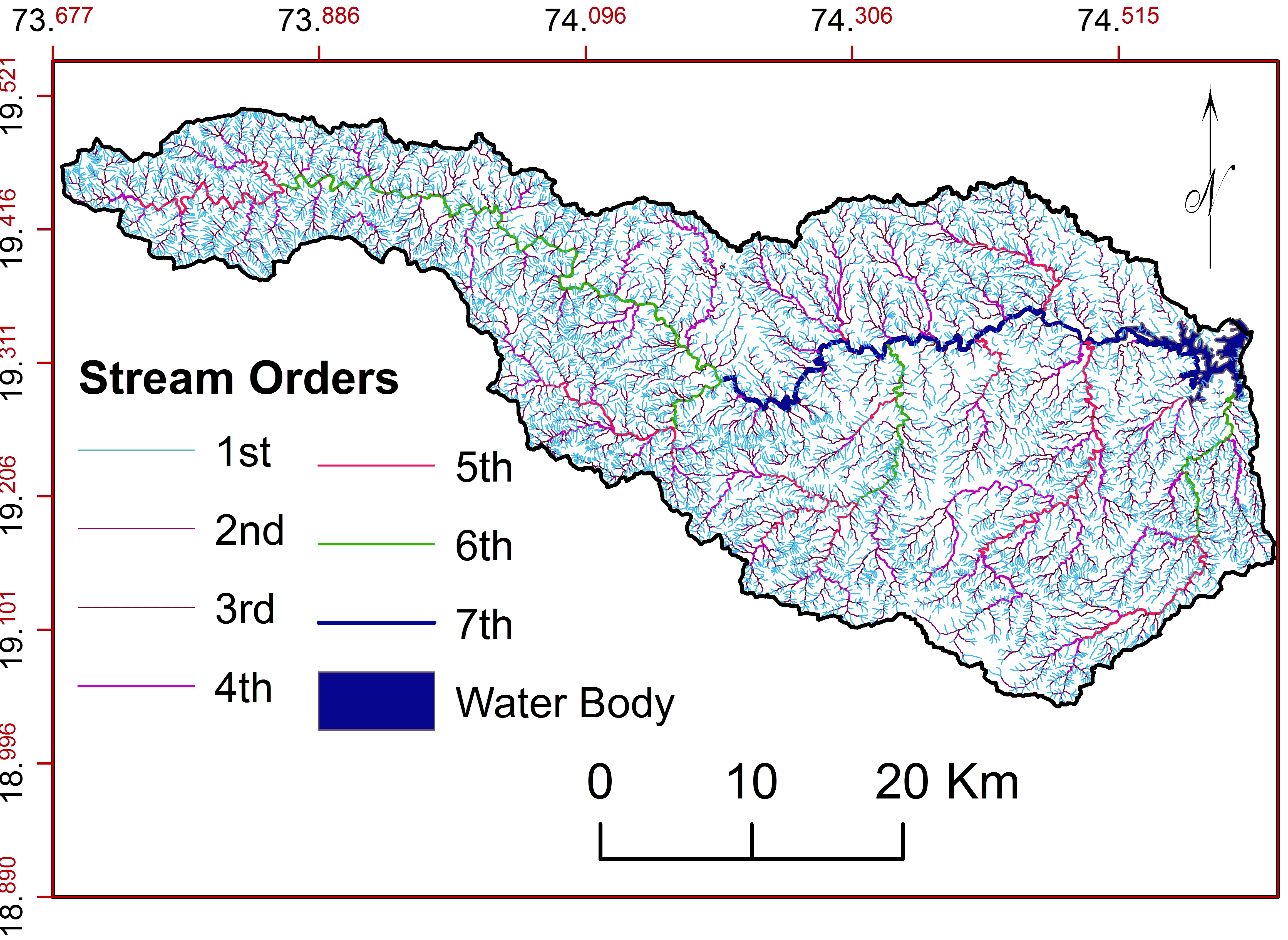
The hierarchical stream ordering is first step of drainage basin analysis (Iqbal and Sajjad, 2014; Raja and Karibasappa, 2016). Lithology, structure and uniformity of rocks in the region can determine using the analysis of stream orders (Shing and Shing, 2011; Vandana, 2013; Chitra et al., 2011; Zende et al., 2013; Ali and Ali, 2014). First order streams in the region are 7682 (69.29 %); second order streams are 2676 (24.14%); third order streams are 554 (5%); forth order streams are 103 (0.93%); fifth order streams are 56 (0.51); sixth order streams are 15 (15%) and seventh order streams is 1 (0.009%) (Figure 5).
b. Mean Stream Length ( \(L_{sm}\) )
\(L_{sm}\) (Equation) is useful to understand the dimensional properties of the drainage basin, size of the drainage network and topography of the basin (Kulkarni, 2015; Iqbal et al., 2013; Singh and Singh, 2011; Pareta and Pareta, 2011). \(L_{sm}\) of the given order is higher than the earlier and lower than the next order (Farhan and Anaba, 2016; Kaur et al., 2014; Rai et al., 2014; Yunus et al., 2014; Aher et al., 2014; Rao and Yusuf, 2013; Mishra and Nagarajan, 2010). It is negatively related with stream frequency, drainage density and length flow (Khare et al., 2014; Rekha et al., 2011). It varies from 0.00 to 2.02 with cumulative \(L_{sm}\) of 0.80km in the basin (Figure 6).
c. Stream Length Ratio \(R_{L}\) )
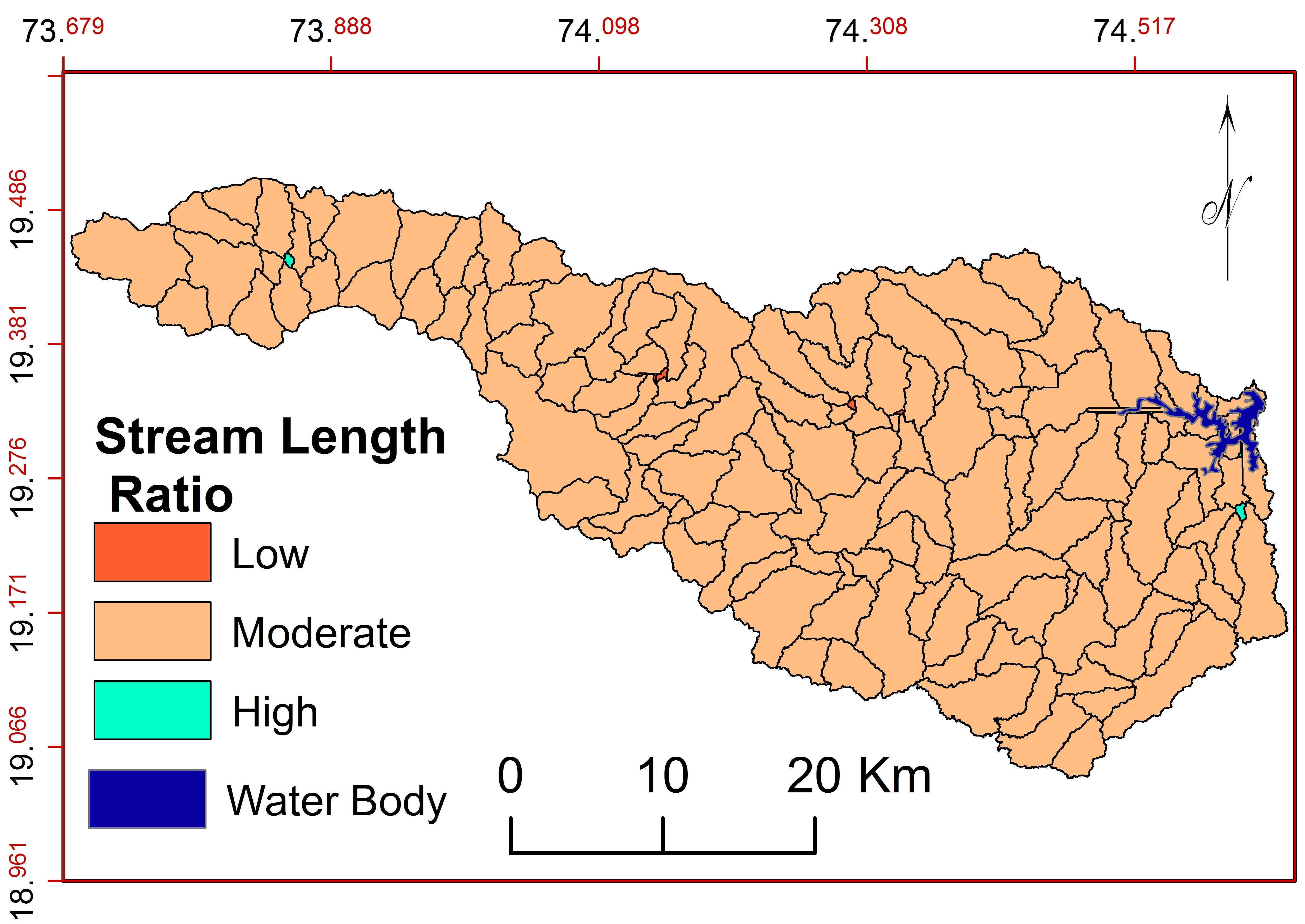
\(R_{L}\) is the ratio of mean length of the stream to the length of the stream from lower order (Khadri and Thakur, 2013; Wilson et al., 2012; Nongkynrih and Husain, 2011; Gray, 1961). \(R_{L}\) shows relationship with bifurcation ratio, surface flow and erosional proses (Gebre et al., 2015; Jagadeesh et al., 2014; Rao and Yusuf, 2013; Iqbal et al., 2013; Rosso and Bacchi, 1991). Sub-watersheds like WS35, WS36, WS52, WS55, WS71 show low \(R_{L}\) and only four sub-watersheds (WS7, WS69, WS72, WS94) show higher \(R_{L}\) (Figure 7). The difference between \(R_{L}\) of 2nd and 4th order streams show high relief and steepness. Therefore, sub-watersheds with moderate \(R_{L}\) can be considered for development and management of resources with priority.
d. Bifurcation Ratio ( \(R_b\) )
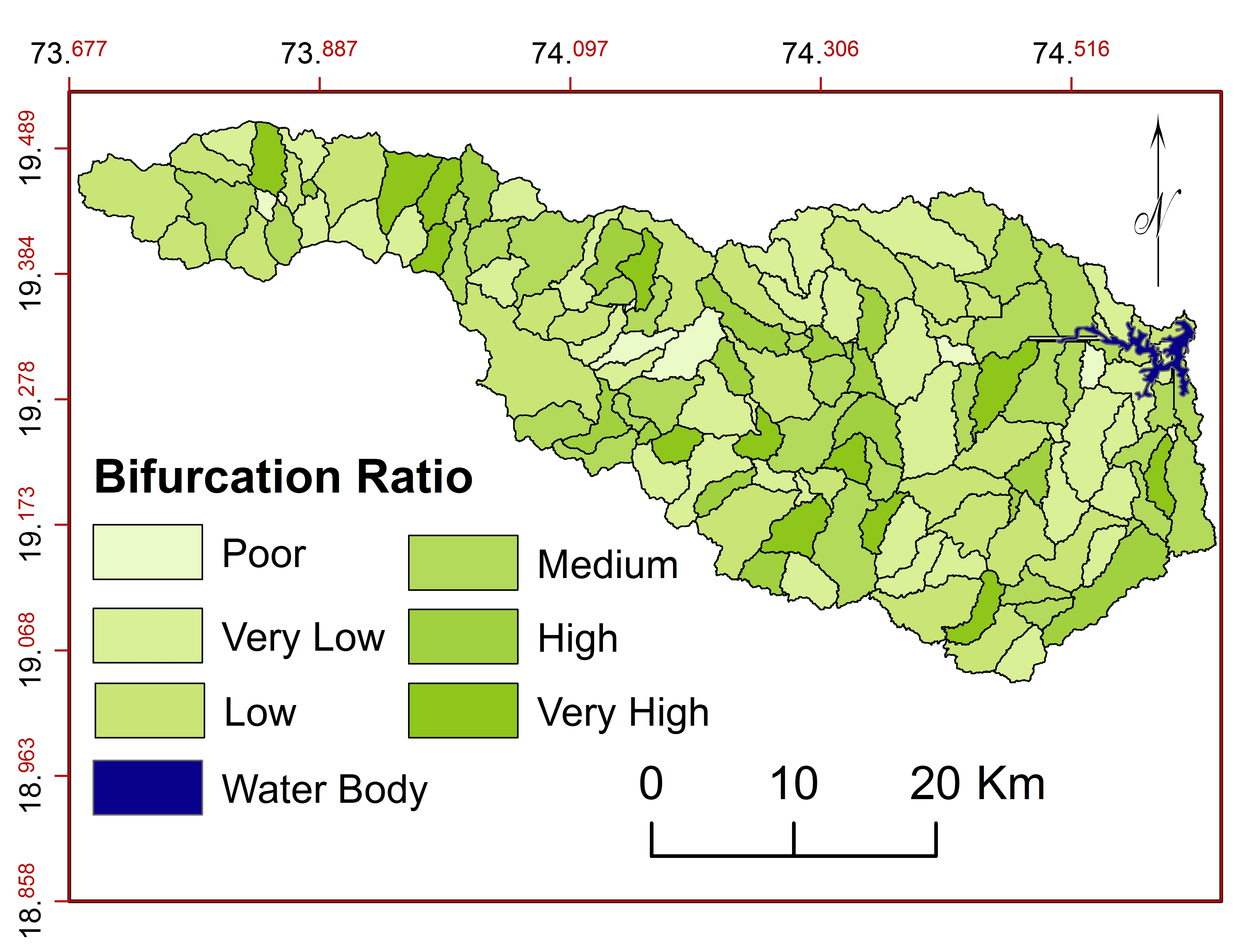
\(R_b\) indicates the shape, pattern and erosion activity in the basin. Higher \(R_b\) indicates an elongated shape of the basin (Chitra et al., 2011; Khare et al., 2014) with more structural control over total drainage system (Chitra et al., 2011) and lower value shows less structural conflicts (Strahler, 1964) with stable drainage (Pareta and Pareta, 2011). \(R_b\) is the ratio of total number of streams of first order to the number of streams from next higher order in the basin (Pareta and Pareta, 2011; Iqbal and Sajjad, 2014). \(R_b\) values in the basin varies from 0.50 to 1.00 with low erosional activity and less troubling drainage pattern (Strahler, 1957; Rai et al., 2014). Sub-watersheds are classified (Figure 8) into six classes: poor (0.1.5), very low (1.5-3.35), low (3.35-3.88), medium (3.88-4.80), high (4.80-6.00) and very high (6.00-9.63) (Rekha et al, 2011).
e. Stream Length ( \(L_u\) )
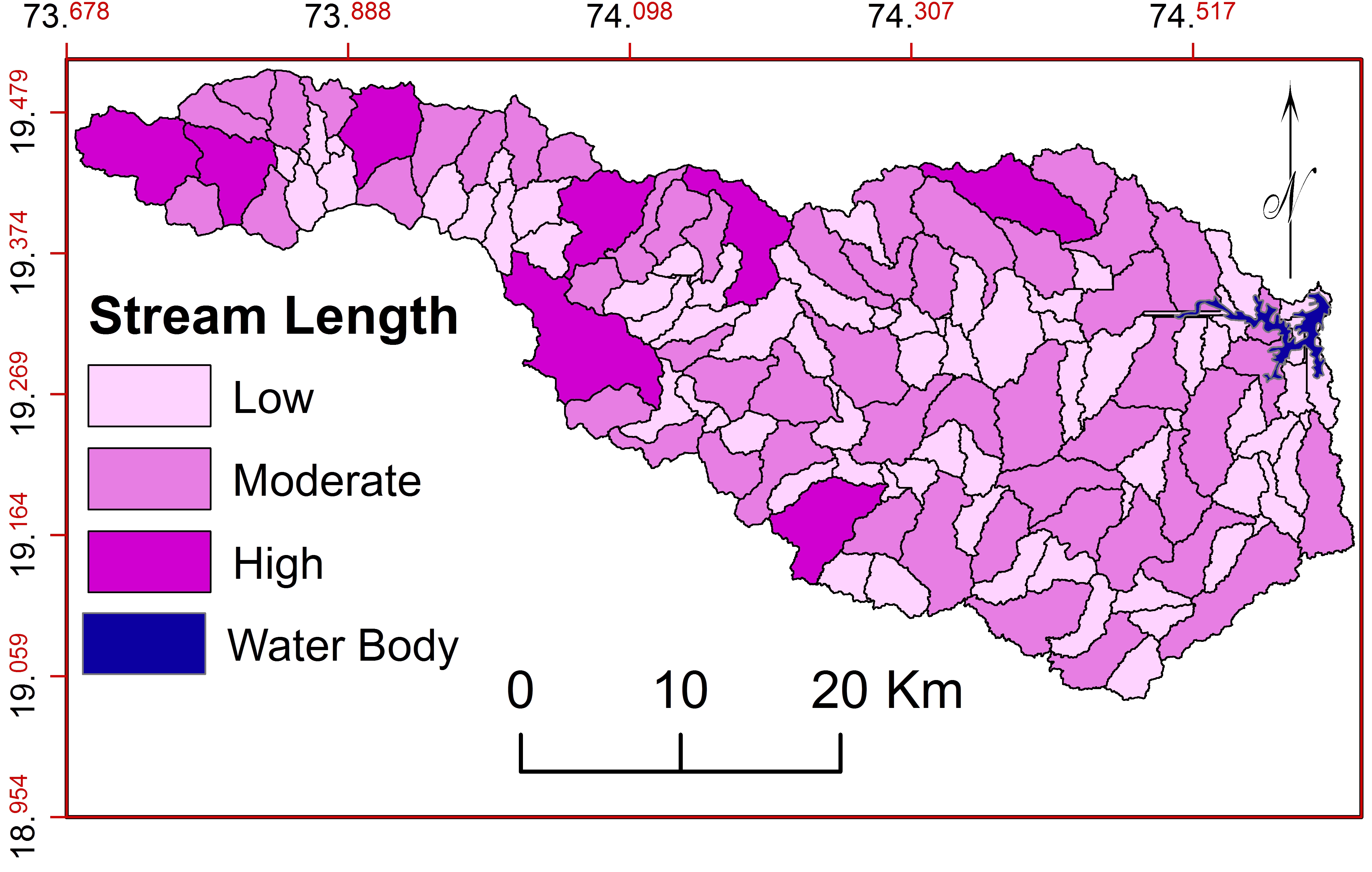
\(L_u\) reveals physical characteristics: lithology, topography and steepness (Nongkynrih and Husain, 2011; Iqbal and Sajjad, 2014). \(L_u\) is measured from topographical maps (Nagal et al., 2014). Longer streams show more permeable bedrock with well-drained network (Kulkarni, 2015). Stream lengths are observed higher for first order and decreases according to increasing stream order. Total length of first ordered streams is measured of 4096.95km (54.80%), second order 1876.33km (25.10%), third order 856.55km (11.46%), fourth order 3.20.5km (4.29%), fifth order 156.99km. (2.10%), sixth order 113.03 km (1.51%) and seventh order 53.57 (0.72%). Stream lengths in the basin are classified (Figure 9) into three classes: low (<49.82), moderate (49.83-123.28) and high (>123.29). Sub-watersheds of 2nd, 3rd and 4th orders are more suitable for soil and water conservation.
3.2.2.2 Aerial Aspects
Areal aspects describe areal elements, law of stream areas, relationship between stream area and stream length, relationship of area to the discharge, basin shape, drainage density, etc. (Aher et al., 2014; Gaikwad and Bhagat, 2017). Therefore, areal aspects: basin area (\(A\)), basin length ( \(L_b\) ), basin perimeter (\(P\)), shape Factor (\(B_{s}\)), drainage density ( \(D_d\) ), stream frequency (\(F_s\) ), form factor ( \(R_f\) ), circularity ratio ( \(R_c\) ), elongation ratio ( \(R_e\) ), compactness coefficient ( \(C_C\)) , drainage texture (\(D_t\) ), texture ratio (\(T\)) and infiltration number ( \(I_{f}\) ) are analyzed for prioritization of sub-watersheds in the basin.
a. Basin Area (A)
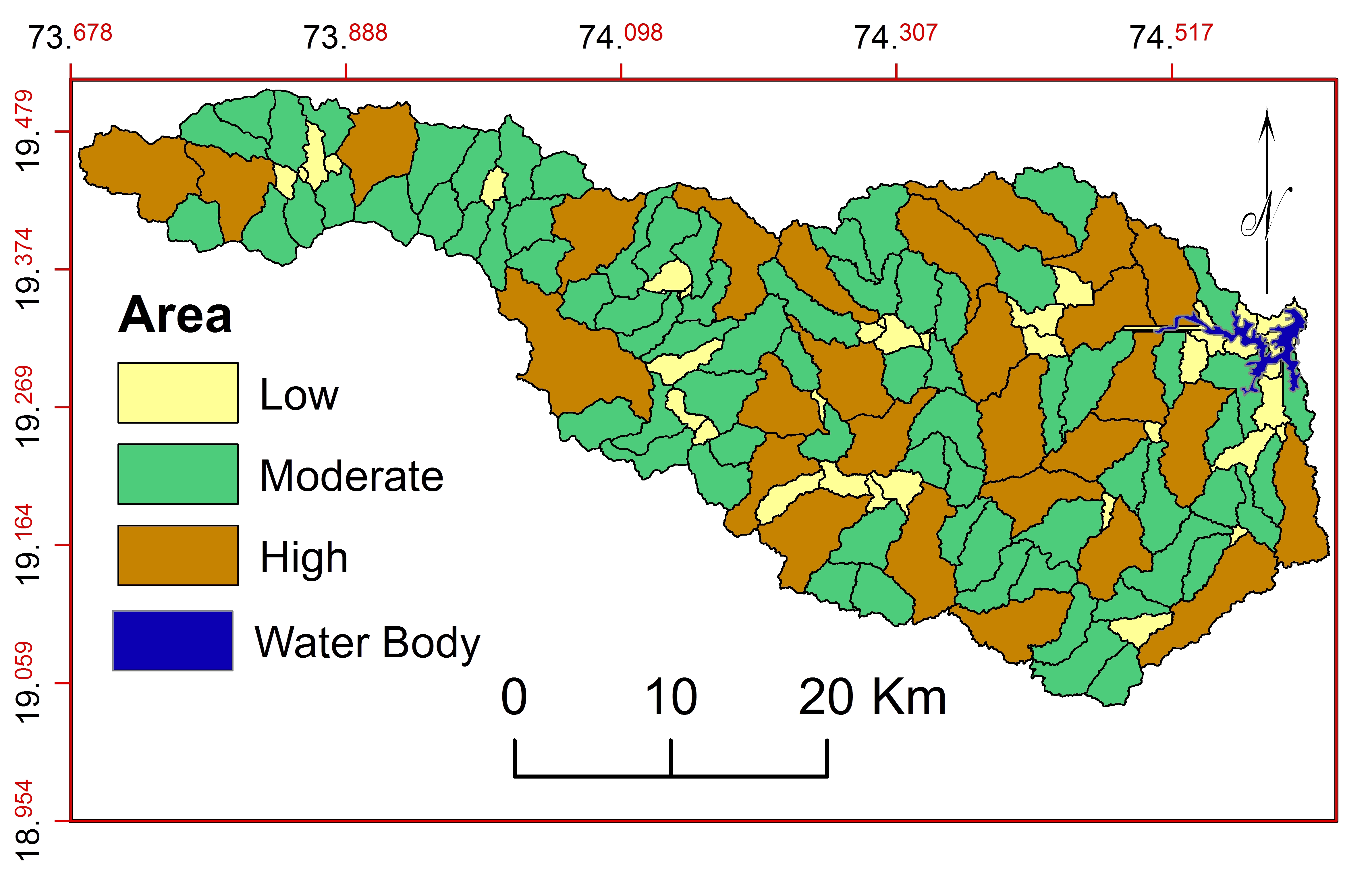
Basin area indicates the size of basin (Strahler, 1957). It is useful to calculate the drainage density (\(D_d\)) stream frequency (\(F_s\)) form factor (\(R_f\)) circularity ratio (\(R_c\)) elongation ratio (\(R_e\)) compactness coefficient (\(C_C\)) and lemniscate’s \(k\) (Gabale and Pawar, 2015). The size of the basin is 2339.7 km2 distributed within 140 sub-watersheds. These watersheds are classified (Figure 10) into three classes: low (<0.19 Km2), moderate (0.19-25.07 Km2) and high (>25.07 Km2).
b. Basin Length ( \(L_b\) )
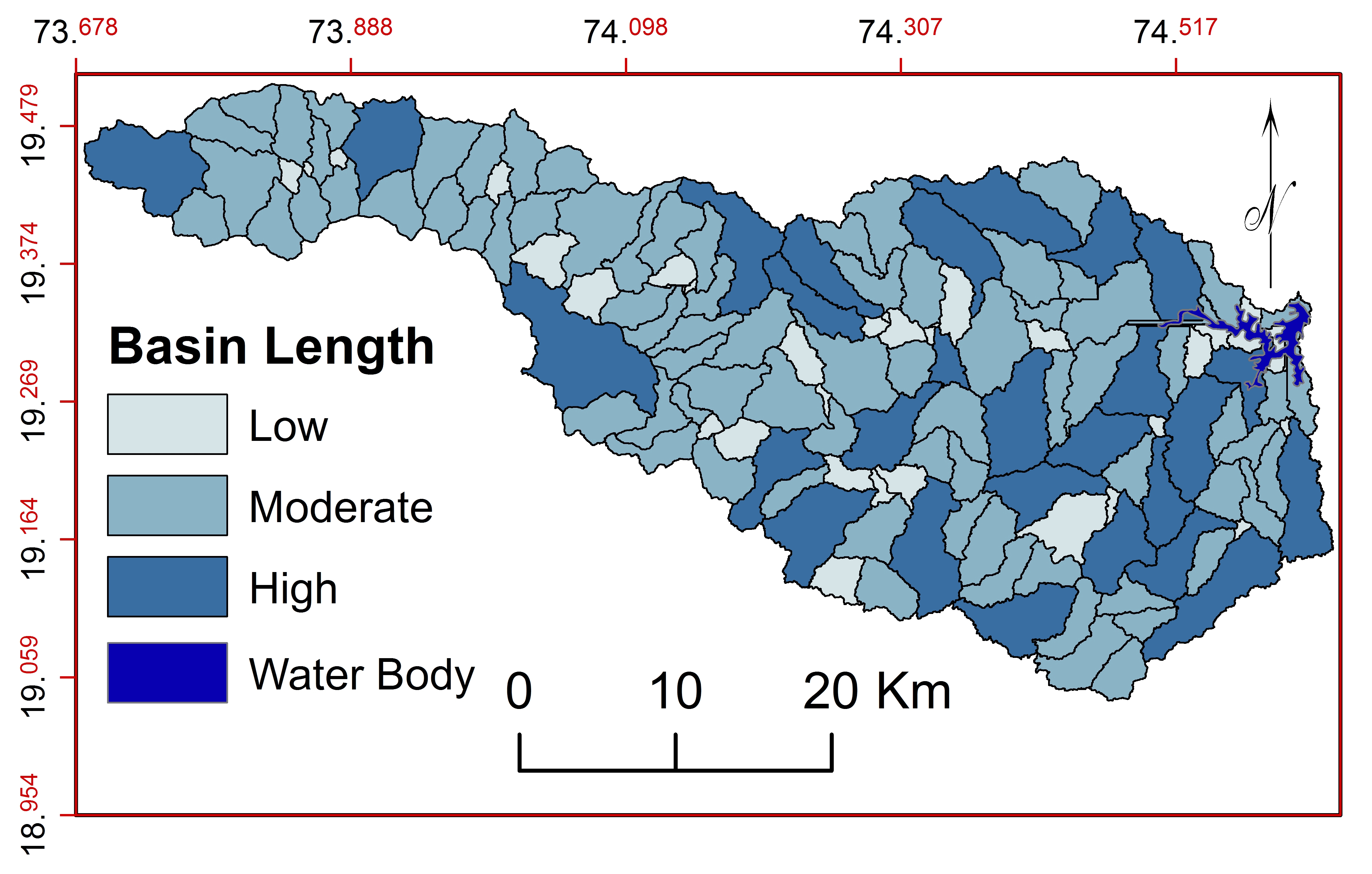
\(L_b\) is useful to understand the basin shape and hydrological characters (Chitra et al., 2011), lemniscate’s value, form factor and elongation ratio of the basin (Pareta and Pareta, 2011). \(L_b\) varies from 1.03 to15km and classified (Figure 11) into three classes: low, moderate and high. Average length of class, ‘low’ is 2.67km, ‘moderate’ is 6.49km and ‘high’ is 11.08km. Moderate values indicate more texture, infiltration number and perimeter relation.
c. Basin Perimeter (\(P\))
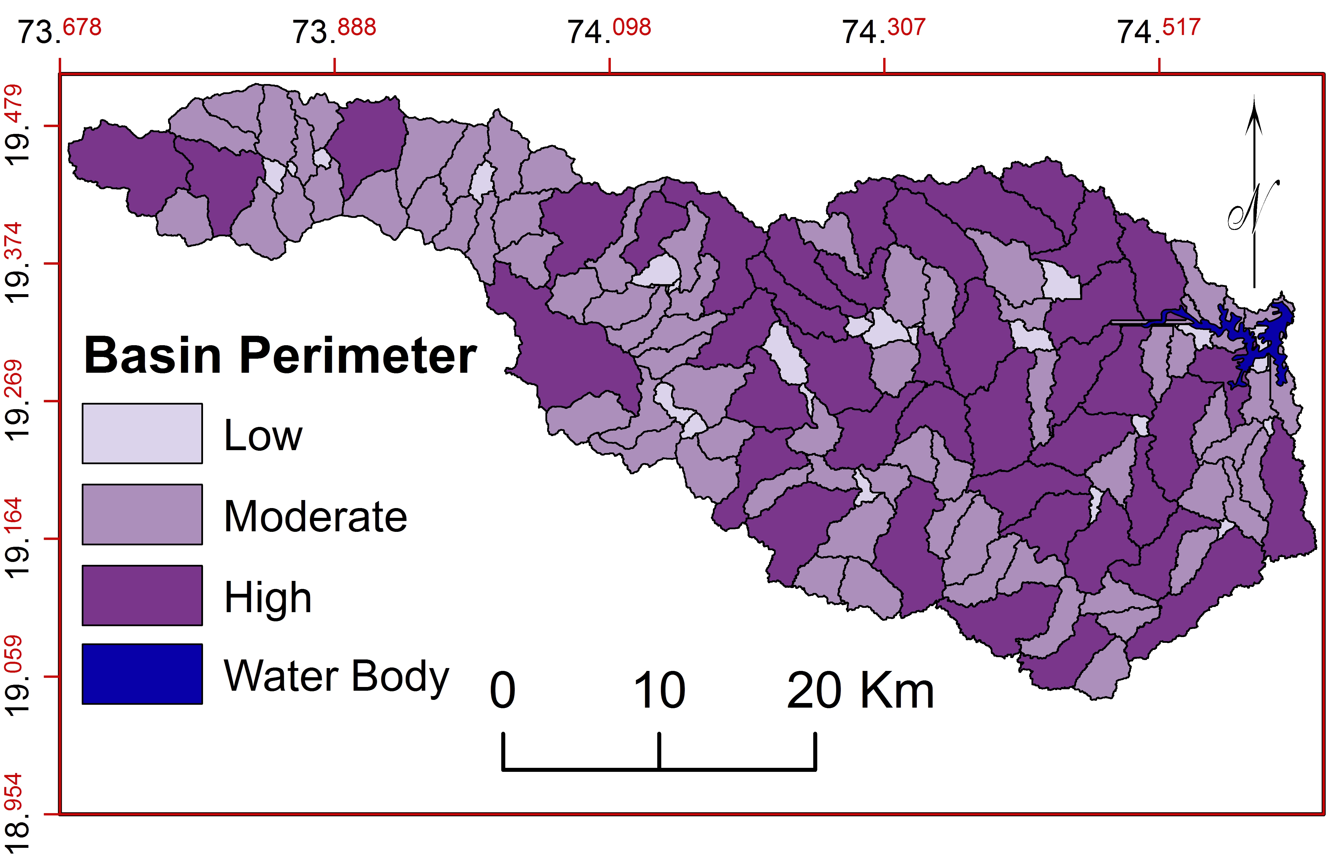
\(P\) is the outer boundary of watershed indicates size, shape and drainage density of the basin (Strahler, 1957). The perimeter of study area is 3901.58km. P of sub-watersheds varies from 7.54km for WS4 to 69.82km for WS87 and classified (Figure 12) into three classes: low (<17.97km), moderate (17.97-33.58km) and high (>33.58km). However, most of the sub-watersheds in the classes: ‘moderate and ‘high’ trends to be elongated with longer duration of low peak flow (Farhan and Al-Shaikh, 2017). 27 sub-watersheds show ‘low’ basin perimeter (11.06km), 72 show ‘moderate’ (25.59km) and 41 show high basin perimeter (42.94km).
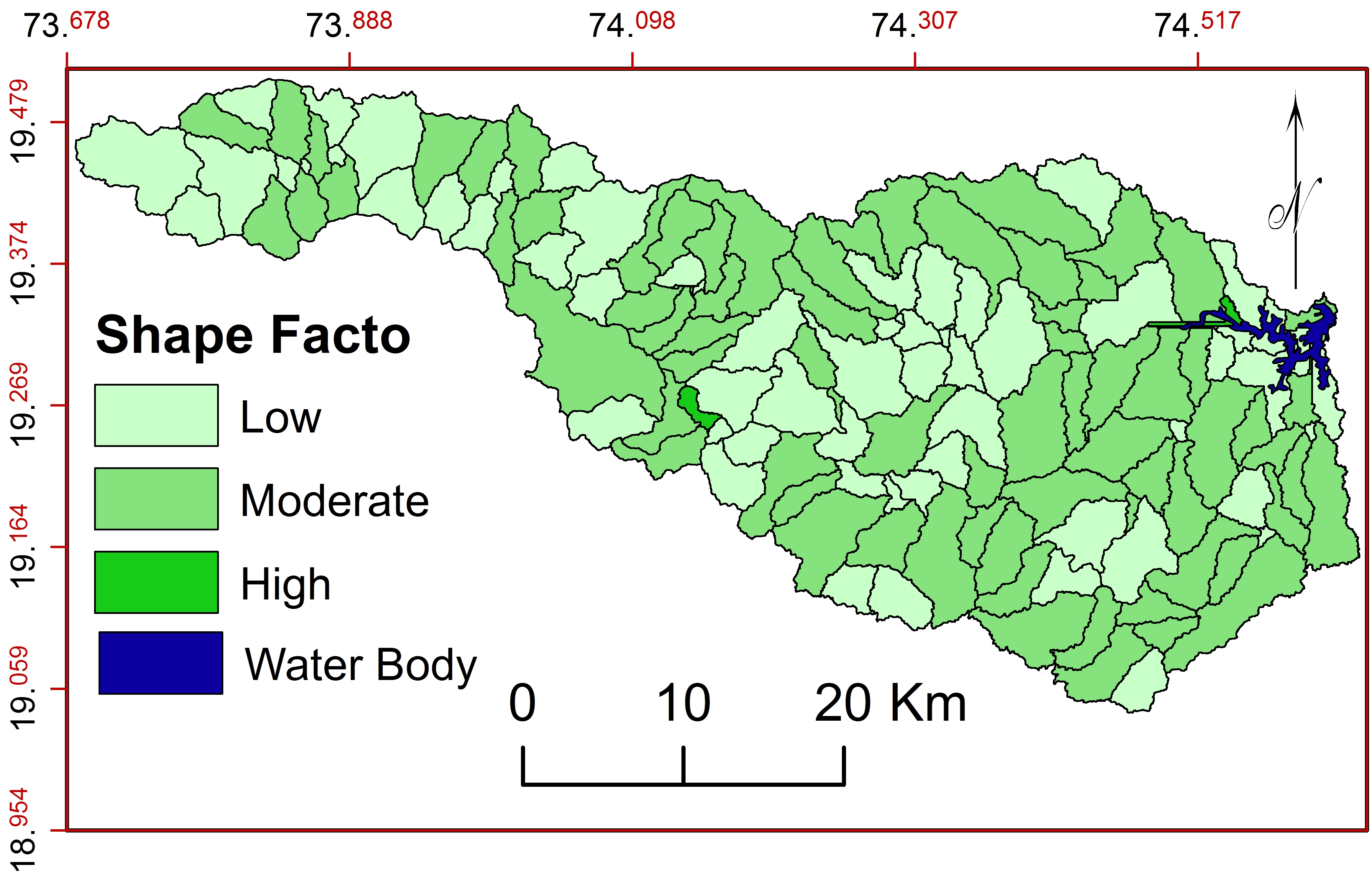
d. Shape Factor (\(B_{s}\))
\(B_{s}\) is the ratio of square of length and area of the basin (Horton, 1945). The calculated values of \(B_{s}\) varies from of 0.05-13.55 (Patel et al., 2013; Sepehr et al., 2017). These values indicate the elongated shape of the basin with flatter peak flow for longer spell (Patel et al., 2013). \(R_f\)\(B_{s}\) is suitable for the morphometric classification of drainage basins. These parameters are controlling the runoff pattern, sediment yield and hydrological condition of the basin (Iqbal et al., 2013, Ali and Ali, 2014). About 63 sub-watersheds show ‘low’ and 74 show ‘moderate’ \(B_{s}\) (Figure 13). The shape of sub-watersheds is elongated and suitable for resource planning and management.
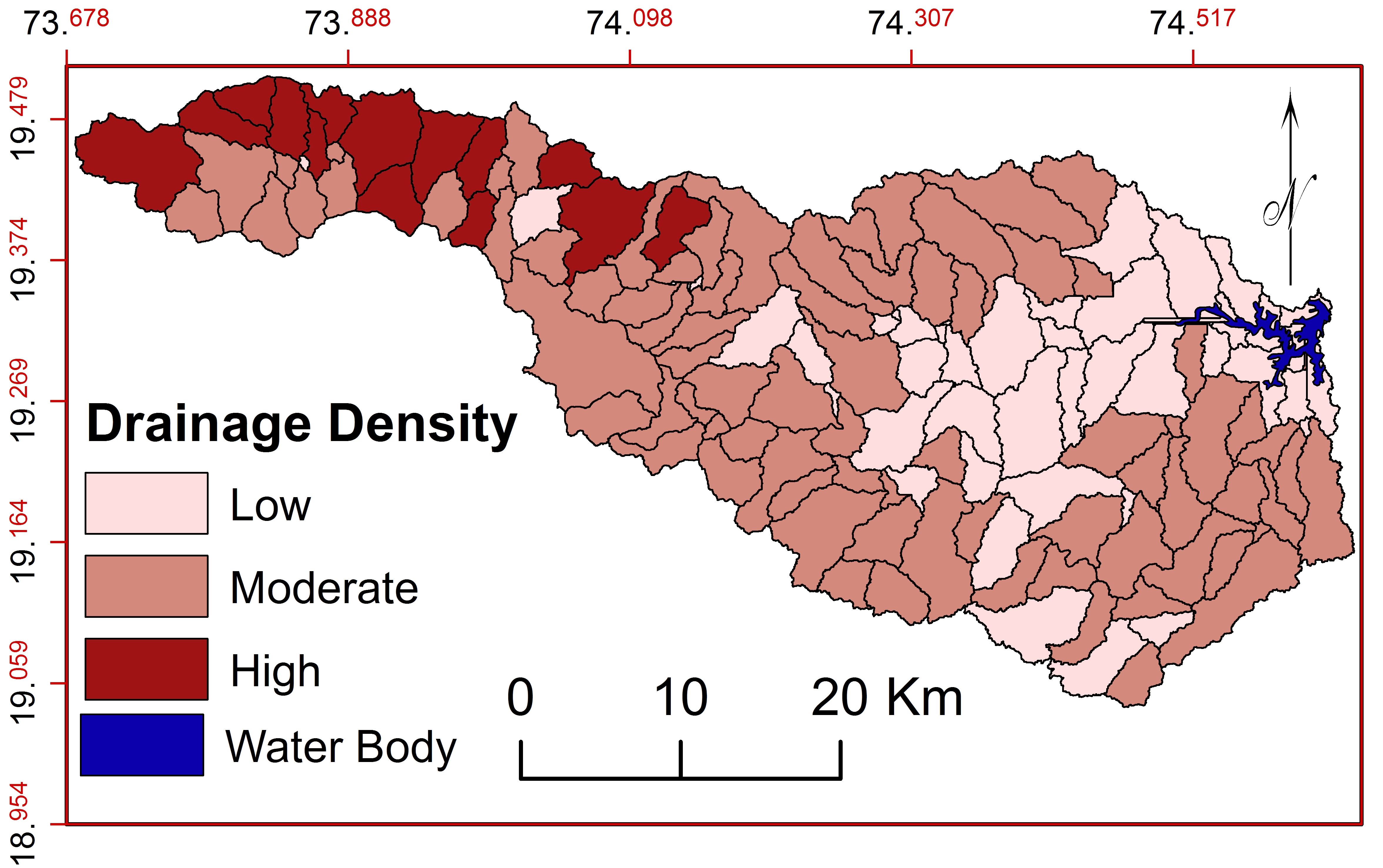
e. Drainage Density ( \(D_d\) )
\(D_d\) is useful to understand the terrain, rocks, relief, soils, groundwater, erodibility and discharge of water and sediment (Pareta and Pareta, 2011; Engelhardt et al., 2012, Kaur et al., 2014; Gebre et al., 2015; Gabale and Pawar, 2015). Higher values of \(D_d\) indicates moderate slopes (Vandana, 2013; Argyriou et al., 2016) with semi-permeable hard rock, coarse textures, favorable conditions for groundwater conservation (Khare et al., 2014; Gebre et al., 2015; Gabale and Pawar, 2015). Gebre and Pawar (2015) have classified \(D_d\) as very coarse from 2.17 to 3.92 km/km2 and moderate for 3.29 km/sq. to 4.18 km/sq. km. Therefore, sub-watersheds in the basin are classified (Figure 14) into three classes: low (0.00-2.69km/sq. km), moderate (2.69-4.22km/sq. km) and high (4.22 -9.80km/sq. km).
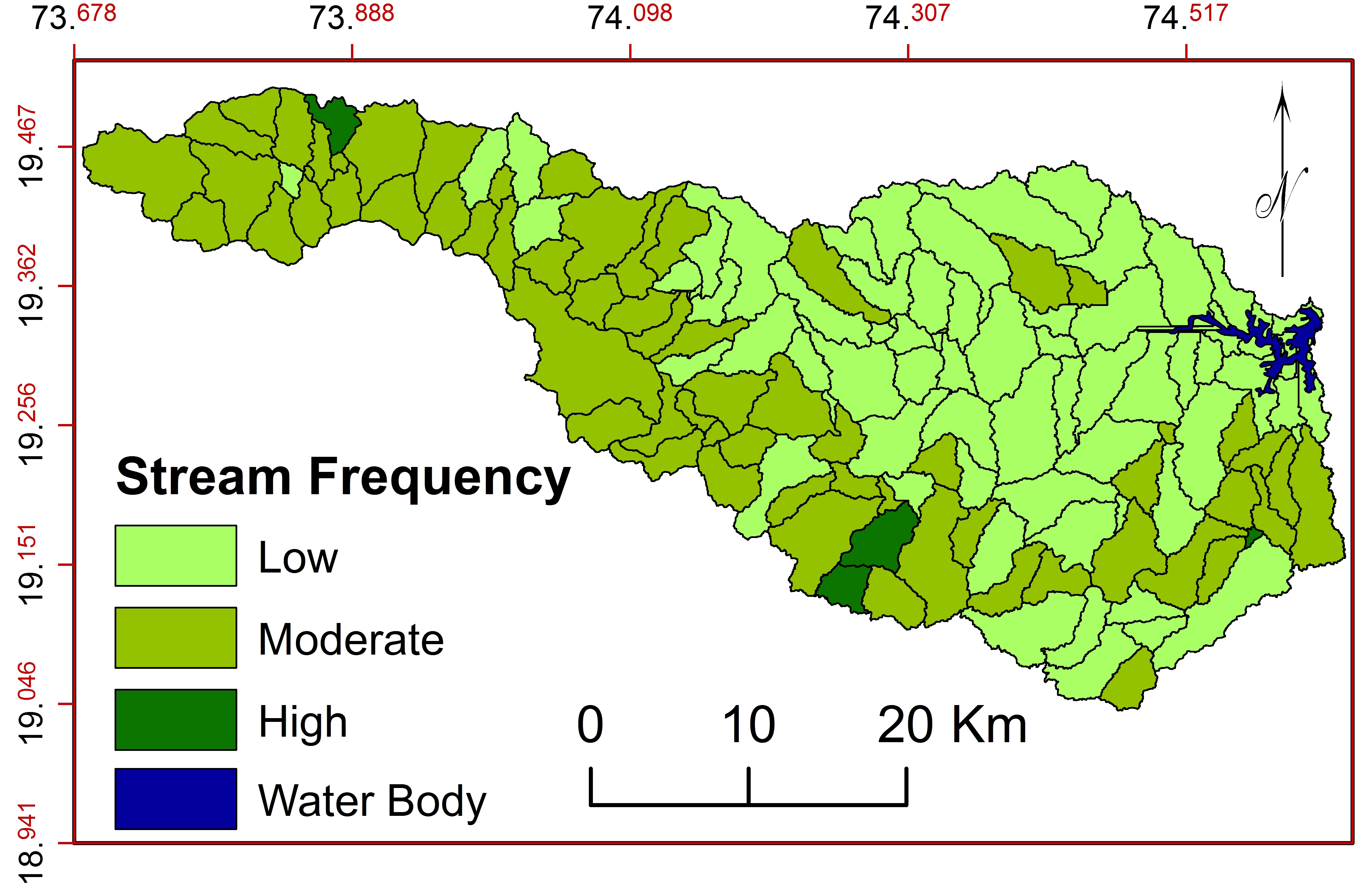
f. Stream Frequency ( \(F_s\) )
\(F_s\) depends on lithology, relief, subsurface permeability, infiltration capacity, drainage network, rainfall, vegetation cover, etc. (Wilson et al., 2012; Aouragh and Essahlaoui, 2014; Gabale and Pawar, 2015; Kulkarni, 2015; Raja and Karibasappa, 2016; Argyriou et al., 2016) therefore, useful to understand physiography, infiltration rate, permeability, number of streams and vegetative cover (Chatterjee and Tantubay, 2000; Pareta and Pareta, 2011; Singh and Singh, 2011; Romshoo et al., 2012; Vandana, 2013; Patel et al., 2013; Iqbal and Sajjad, 2014; Rai et al., 2014; Kaur et al., 2014; Farhan and Al-Shaikh, 2017). Stream frequency in the region varies from 1.52 to 14.53km/km2. Sub-watersheds are classified (Figure 15) into three classes: low (<4.07), moderate (4.07-8.23) and high (>8.23). Higher stream frequencies of WS2 (13.90), WS121 (9.09), WS 127 (8.98) and WS129 (14.53) indicate impermeability and less infiltration capacity of subsurface and higher relief with thin vegetation cover. Sub-watersheds with dense forest show less frequency of streams whereas agricultural lands show higher frequency (Zende et al., 2013).
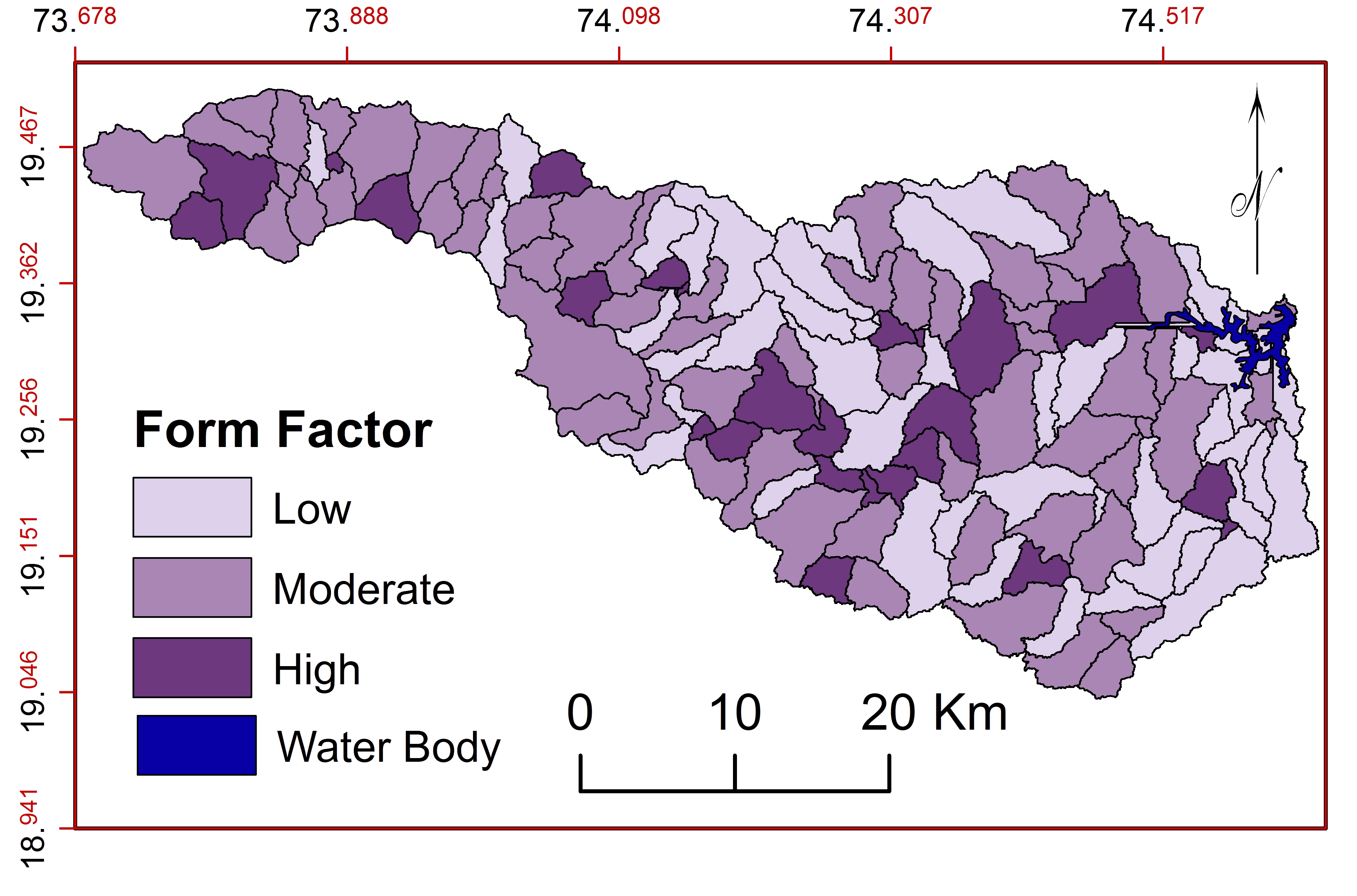
g. Form Factor ( \(R_f\) )
\(R_f\) shows the shape (Rai et al., 2014) and basin length (Patel et al., 2013). The elongated watershed estimates less value and nearly circular watersheds show the higher ( \(R_f\) =0.75) (Gabale and Pawar, 2015) (Figure 16). \(R_f\) for sub-watersheds in the basin varies from 0.07-0.78. Out of them 31 sub-watersheds show elongated shapes with longer duration of flow and 81 sub-watersheds are moderate elongated shaped with moderate peak flow. These elongated and moderate elongated sub-watersheds are suitable for natural resource management. 28 sub-watersheds has near circular shape indicates high peak flow of shorter duration. Moreover, these sub-watersheds are not suitable for natural resource management.
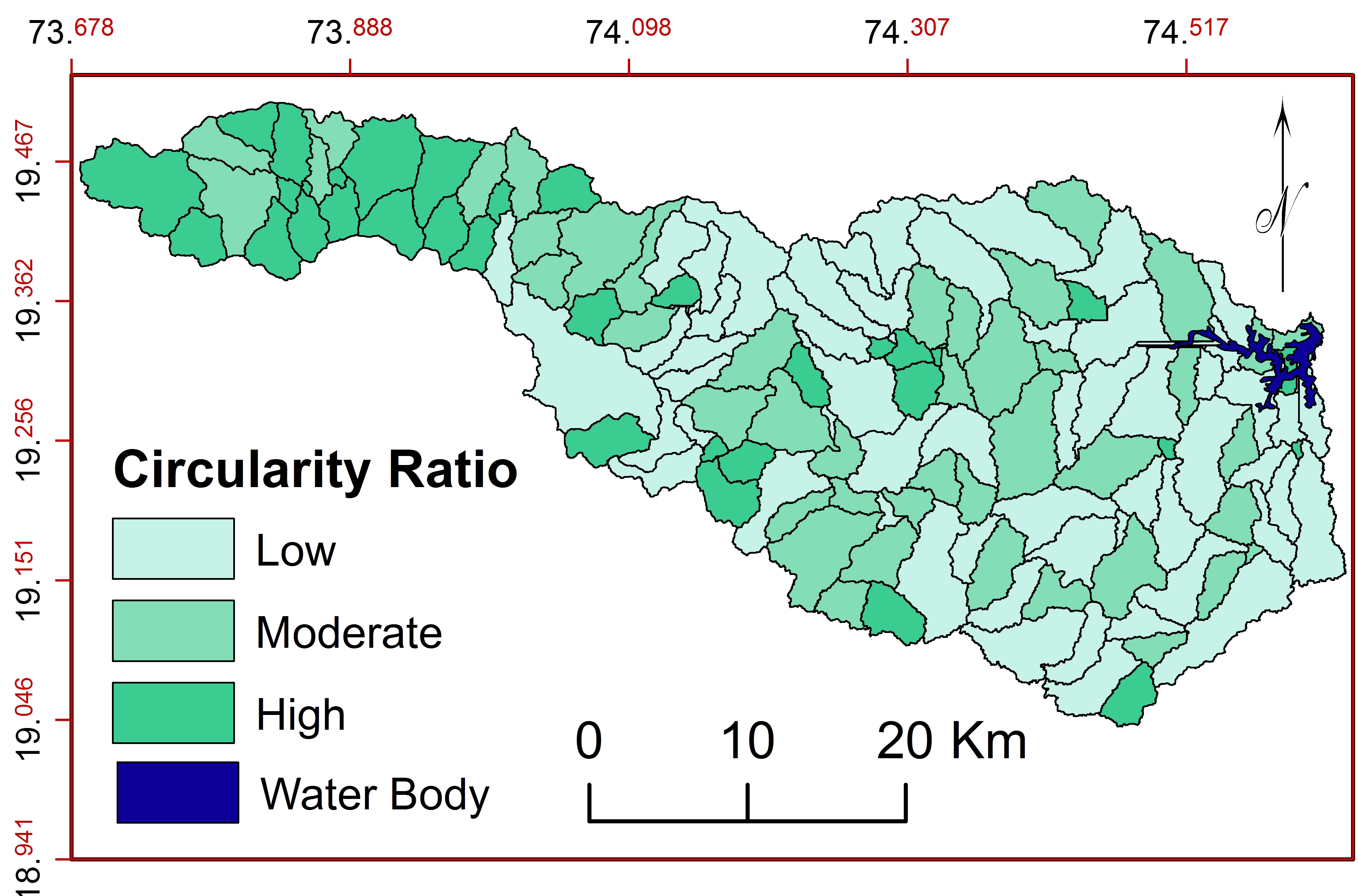
h. Circularity Ratio ( \(R_c\) )
\(R_c\) shows amount of discharge, erosion activity (Patel et al., 2013; Rao and Yusuf, 2013) and nature of topography (Gray, 1961; Ali and Ali, 2014; Farhan and Anaba, 2016). \(R_c\) is dependent on length and frequency of tributaries, geology, relief, climate, land use/land cover, etc. of the region (Mishra and Nagarajan, 2010; Nongkynrih and Husain, 2011; Iqbal et al., 2013; Kaur et al., 2014). Estimated \(R_c\) (0.30 to 0.54) for sub-watersheds show higher erosion activity with permeable homogeneous geology (Aravinda and Balakrishna, 2013; Wilson et al., 2012). These sub-watersheds are classified (Figure 17) into three classes: low (0.08-0.22), moderate (0.22-0.30 and high (0.30-0.54). Sub-watersheds with low and moderate \(R_c\) show young and progressive stages of landform and prone to more erosion.
i. Elongation Ratio ( \(R_e\) )
\(R_e\) is the ratio of diameter and the maximum length of the basin (Nongkynrih and Husain, 2011; Strahler, 1964) and show slope, shape of basin, hydrology, rate of infiltration and runoff (Kaur et al., 2014; Iqbal and Sajjad, 2014; Zende et al., 2013; Wilson et al., 2012, Mishra and Nagarajan, 2010). Higher \(R_e\) shows more infiltration capacity of land with less runoff (Iqbal and Sajjad, 2014. Calculated \(R_e\) are classified into three classes: low (0.31-0.76), moderate (0.76-1.36) and high (1.36-4.83) (Figure 18). Sub-watersheds with higher relief and steep slopes should be selected for conservation purpose with high priority. 93 sub-watersheds are elongated with higher relief and steep slopes and 45 sub-watersheds shows moderate relief with moderate slope. Therefore, sub-watersheds from low and moderate classes are suitable for watershed management.
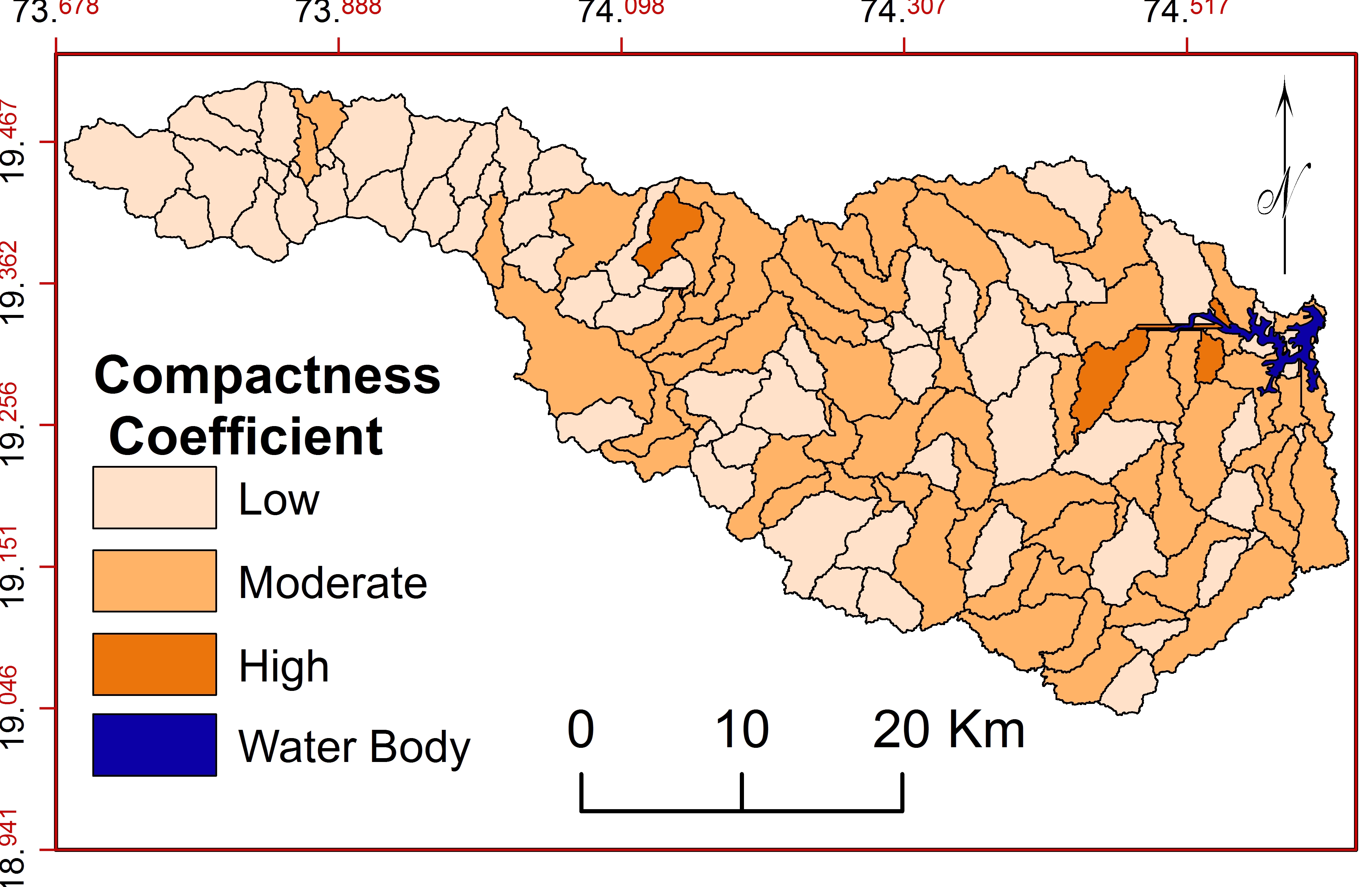
j. Compactness Coefficient ( \(C_C\) )
\(C_C\) is depend on size and slopes in the basin and useful to understand risk of erosion with their hydrologic relationship (Ali et al., 2014; Iqbal et al., 2013; Patel et al., 2013). Estimated \(C_C\) vary from 1.60 to 2.48 (Figure 19) and classified into three classes: low (1.60-1.67), moderate (1.67-1.90) and high (1.90-2.48). Low \(C_C\) values indicate more elongation and higher erosion in the basin (Farhan and Al-Shaikh, 2017). 67 sub-watersheds show low \(C_C\) with more elongation and higher erosion whereas 06 sub-watersheds show low elongation and less erosion. Therefore, low and moderate sub-watersheds are suggested for watershed management.
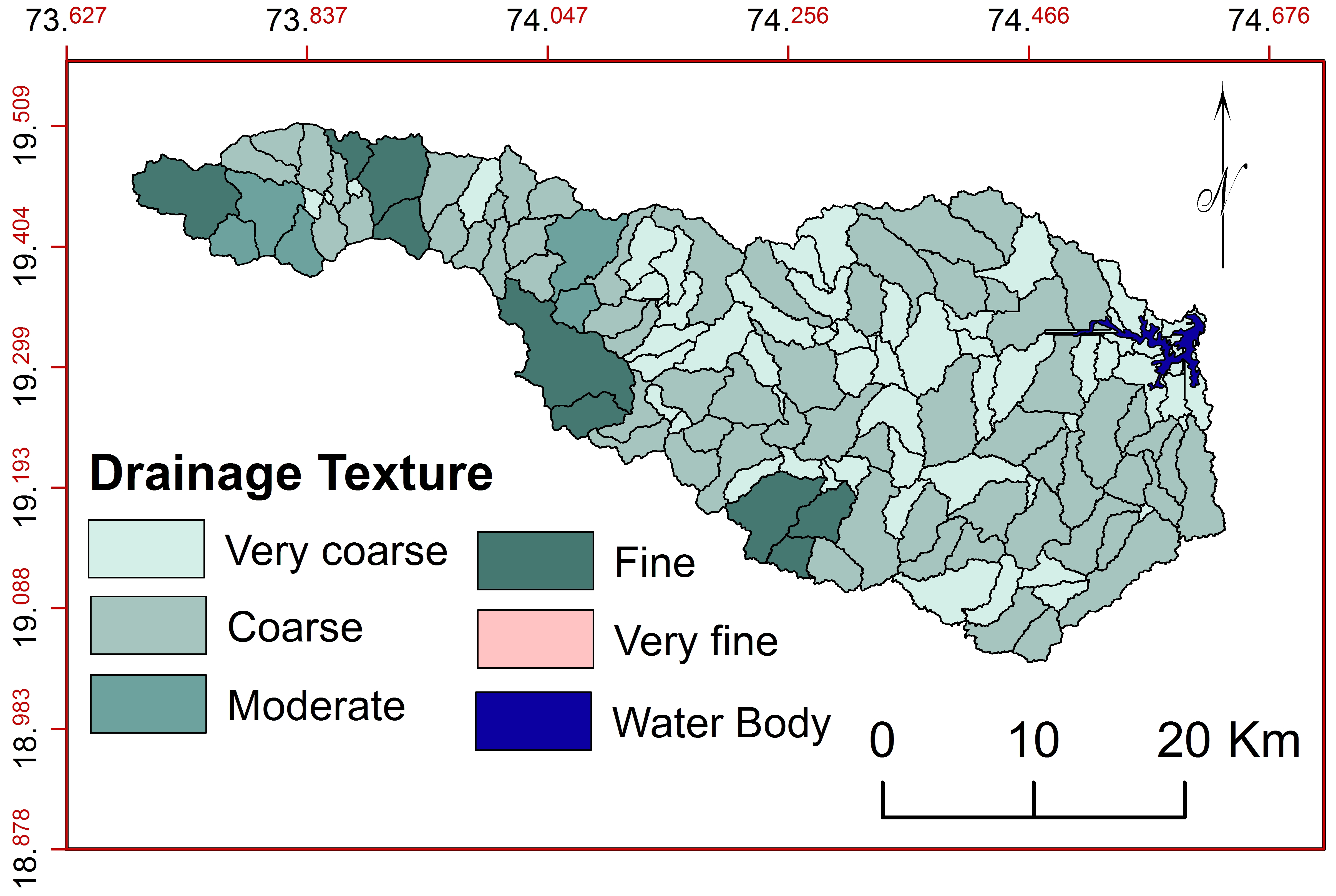
k. Drainage Texture ( \(D_t\) )
\(D_t\) values show lithology (Rao and Yusuf, 2013) and depend rock, soil, infiltration capacity, relief, climate, vegetation, etc. (Kulkarni, 2015; Vandana, 2013; Iqbal et al., 2013; Chatterjee and Tantubay, 2000). 71 sub-watersheds in the basin show very coarse drainage textures with hilly terrain showing steep crumbs and 55 sub-watersheds observed coarse drainage textures with massive and resistant rock structures (Figure 20). Therefore, sub-watersheds with very coarse and coarse drainage textures are suitable for watershed and resource management.
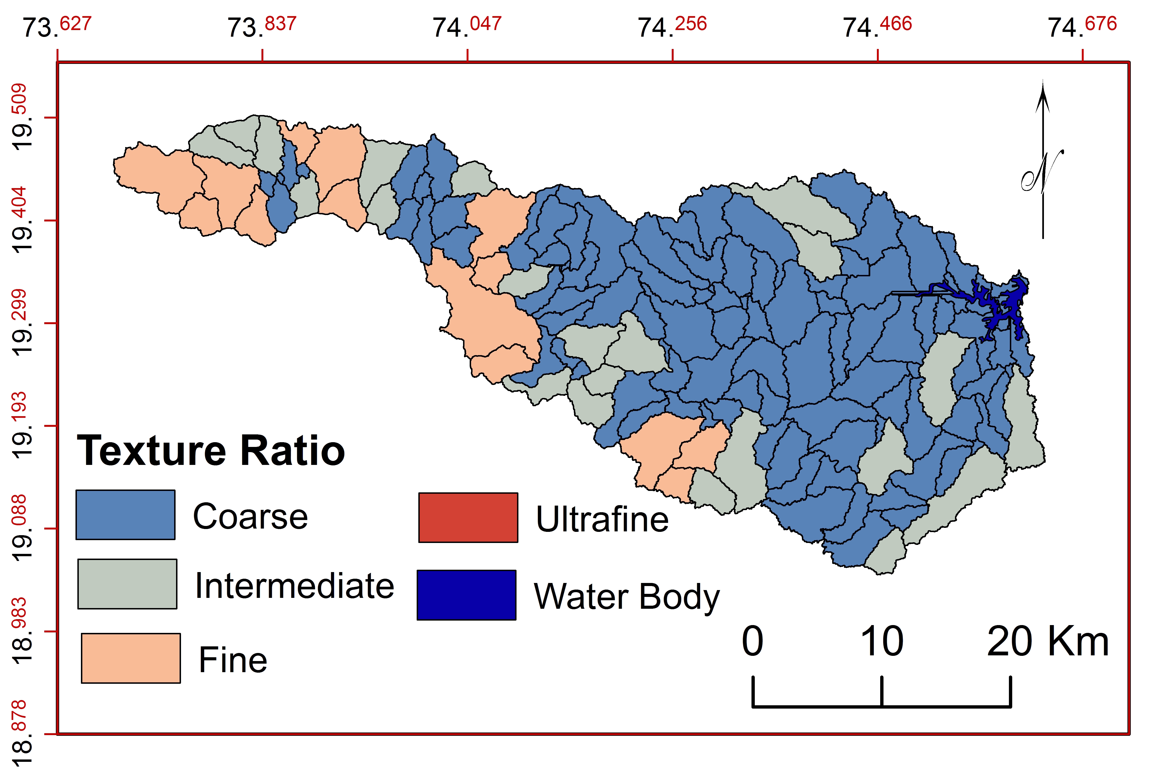
l. Texture Ratio (\(T\))
The values of T estimated for the basin indicate morphometry, runoff and texture of basin (Farhan and Anaba, 2016) and depends on the lithology, infiltration capacity and relief (Khare et al., 2014, Rekha et al., 2011, Pareta and Pareta, 2011). Smith (1950) has classified calculated values of T into four categories: coarse (0-4), intermediate (4-10), fine (10-15) and ultra-fine (>15). Calculated T (Figure 21) in the basin varies from 0.11 (SW74) to 10.55 (SW52). 126 sub-watersheds are unaffected and covered by massive bolder. The group, ‘intermediate’ includes 13 sub-watersheds with classic densities and weathered rocks, therefore these regions are favorable for resource management.
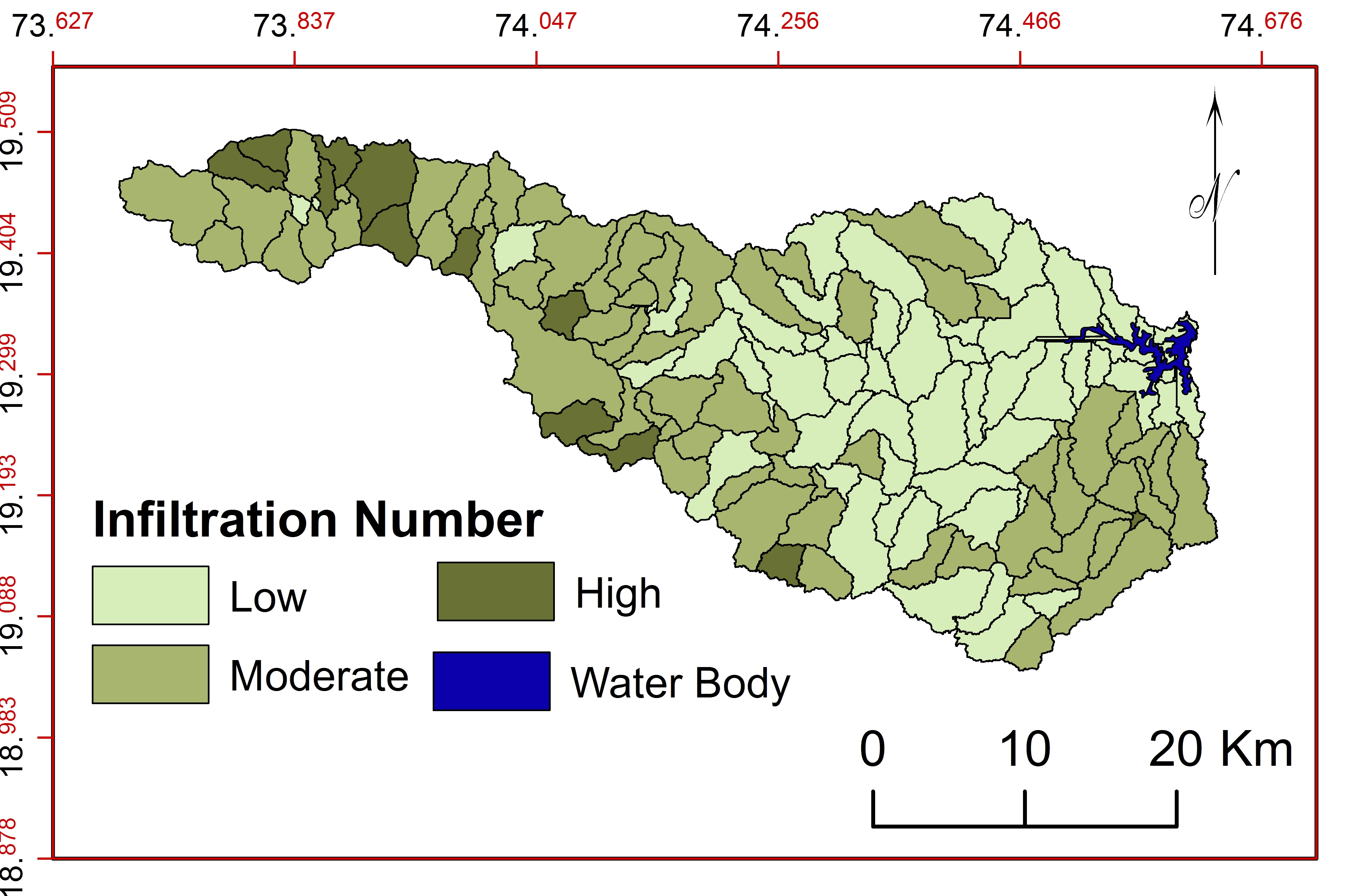
m. Infiltration Number ( \(I_f\) )
\(I_f\) of watershed can be defined as the product of drainage density and stream frequency. \(I_f\) indicates infiltration characters, runoff, vegetation cover and permeability of the land surface (Rao and Yusuf, 2013; Ranjan, 2013; Singh and Singh, 2011). Estimated values of \(I_f\) vary from 0.0 to 72 and classified into three classes: low, moderate and high (Figure 22). 63 sub-watersheds show low \(I_f\) indicating highly permeable soil materials under dense vegetation and 65 sub-watersheds show moderate \(I_f\) with favorable conditions for gully erosion and high runoff.
3.2.2.3 Relief Aspects
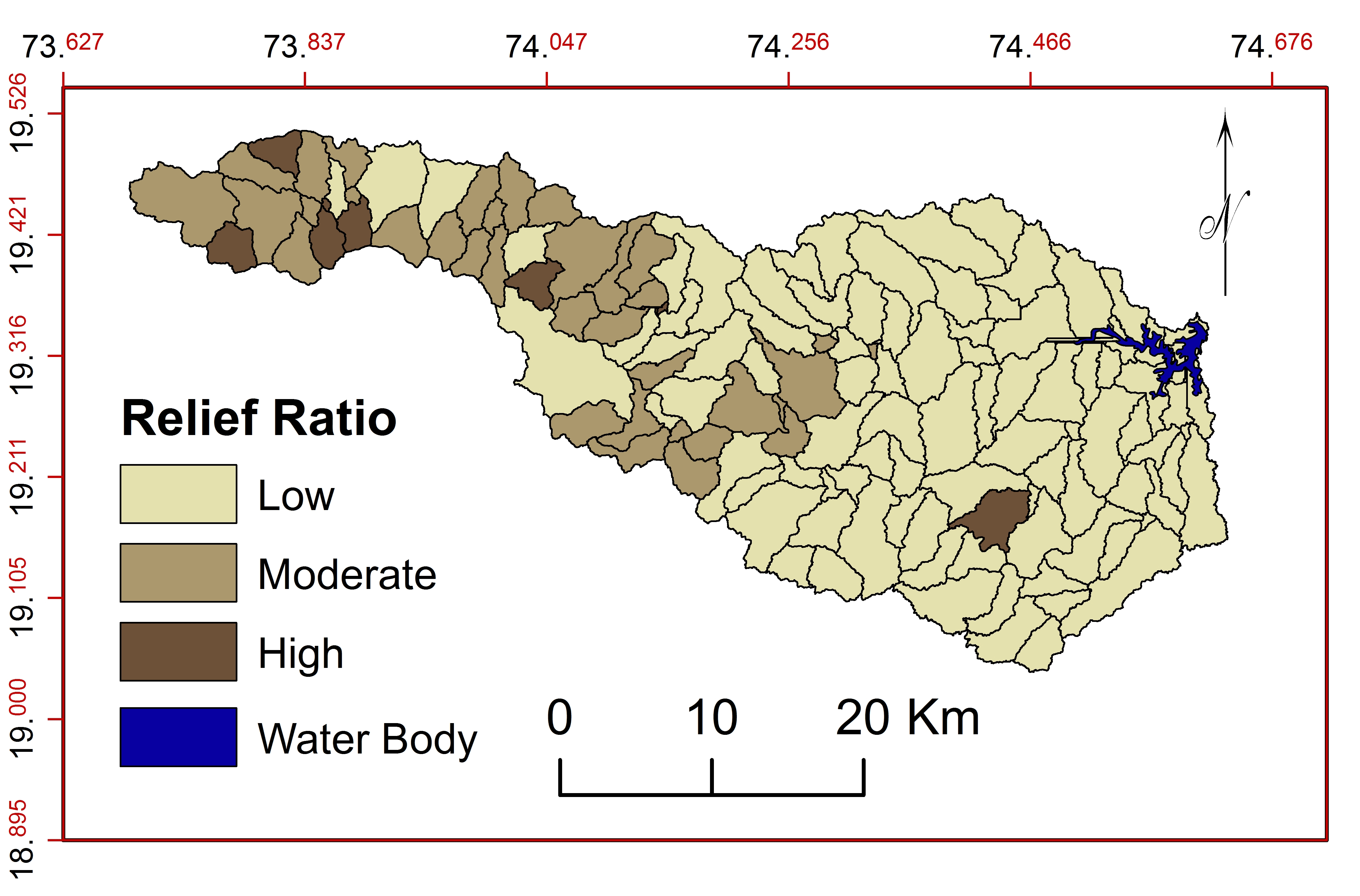
a. Relief Ratio ( \(R_{h1}\) )
\(R_{h1}\) is useful to understand slope, relief and erosion activity in the basin (Strahler, 1957; Sharma et al., 2009; Engelhardt et al., 2011; Wilson et al., 2012; Vandana, 2013; Kaur et al., 2014; Yunus et al., 2014). It is the ratio between the total relief and the longest dimension of the basin. Calculated \(R_{h1}\) vary from 7.84 to 322.70. \(R_{h1}\) normally increases with decreasing drainage area and size of the basin. 94 sub-watersheds show low \(R_{h1}\) (7.84 to 42.64) indicates presence of base rocks, overall steepness and intensity of erosion and 37 sub-watersheds show moderate \(R_{h1}\) (42.64 to 107.60) with moderate slopes, gentle relief and moderate erosion. 9 sub-watersheds in the region show high \(R_{h1}\) (107.60 to 322.70) with steep slopes, brushy vegetation and thin soils (Patton and Baker, 1976) (Figure 23).
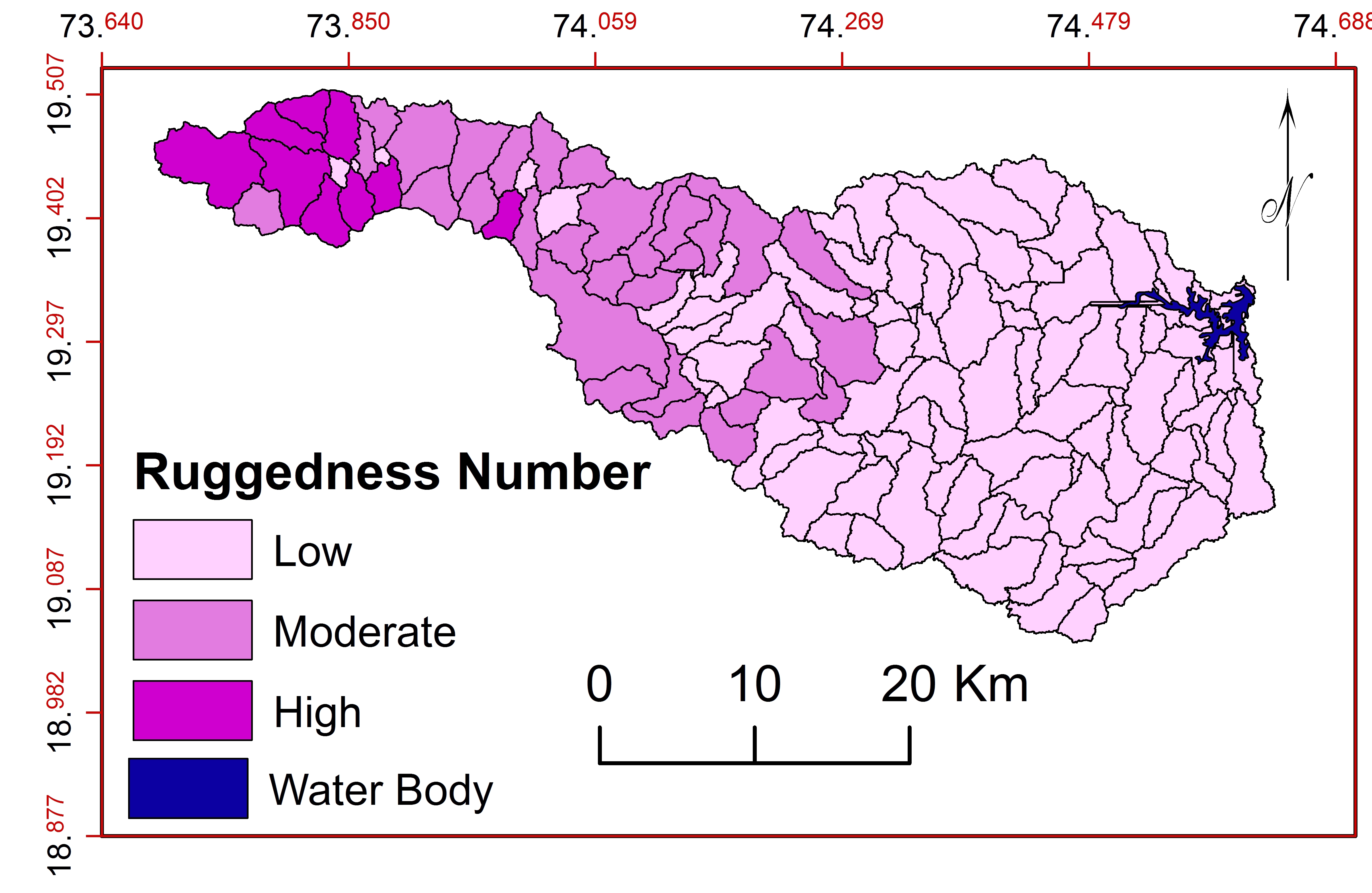
b. Ruggedness Number ( \(R_n\) )
\(R_n\) is the product of basin relief and drainage density and useful to understand the relationship with steepness and length (Kaur et al., 2014). \(R_n\) shows relief, drainage density, slope, soil erosion and discharge (Pareta and Pareta, 2011; Rao et al., 2004; Nagal et al., 2014; Gaikwad and Bhagat, 2017). Calculated \(R_n\) values are classified into three classes: low, moderate and high (Figure 24). 89 sub-watersheds show low ruggedness values (0.00 to 908.84) with irregular topography, lithological heterogeneity, high drainage density and high soil erosion. 42 sub-watersheds show moderate value (908.84 to 2204.45) with flat surface, valley topography and moderate to moderately high degree of dissection and moderate to soil erosion and 9 sub-watersheds show high value (2204.45 to 4734.21) with very steep slopes and more peak discharges flows.
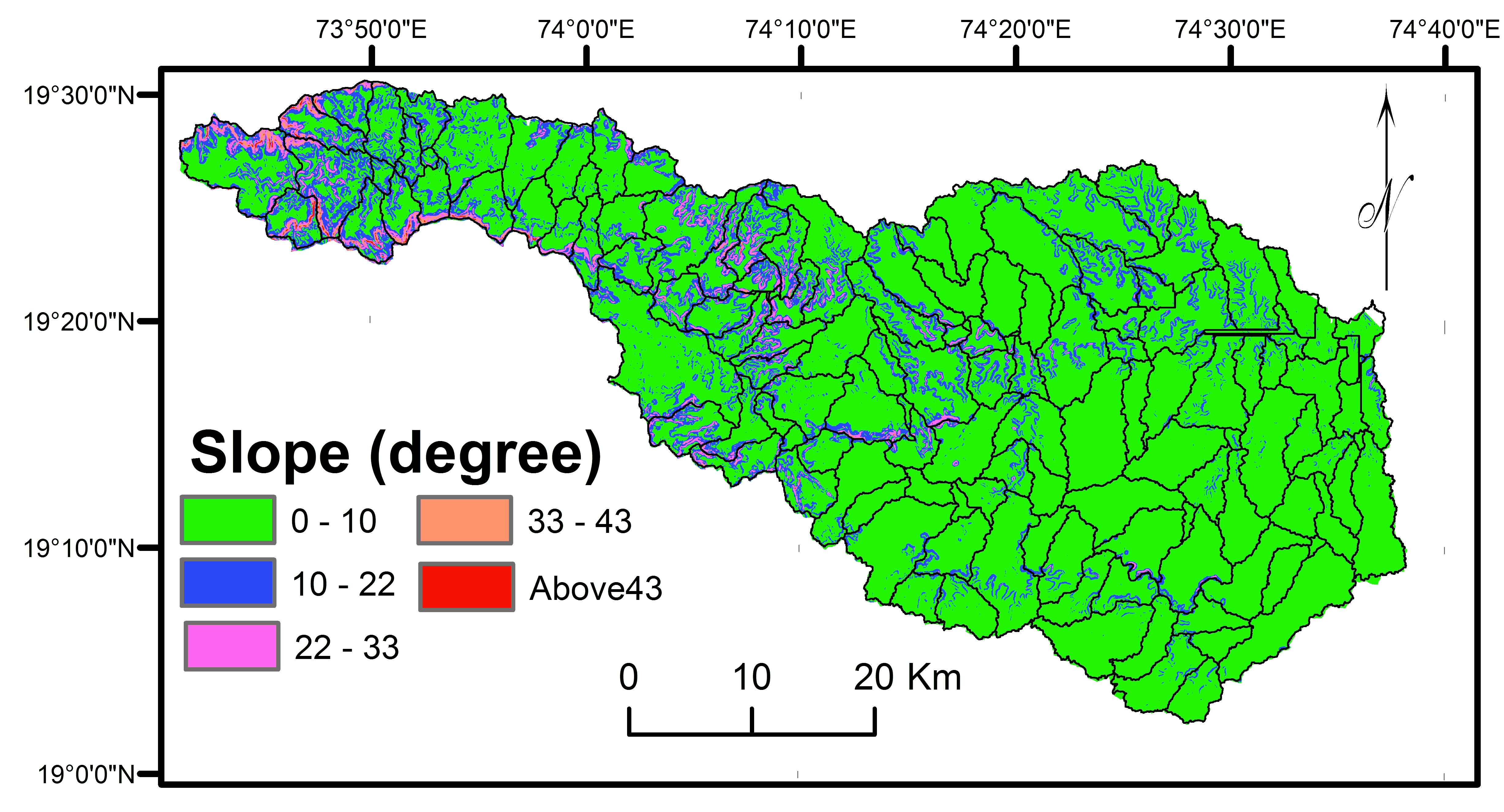
c. Slope
The slope analysis is useful to detect suitable sub-watersheds for planning and management for development (Zolekar and Bhagat, 2015; Argyriou et al., 2016). Slopes in the basin play key role in runoff formation, infiltration rate (Sepehr et al., 2017), flow density (Kaur et al., 2014; Rekha et al., 2011; Wilson et al., 2012), floods and erosion. Water can be stored at the bottom of the valley with gentle slopes (Emamgholi et al., 2007). Slope determines the soil depth, vegetation cover, ground water recharge, surface runoff, etc. (Shinde et al., 2010; Zolekar and Bhagat, 2015; Khare et al., 2014; Rezaei et al., 2013; Rekha et al., 2011). Sub-watersheds with moderate slopes (10º-22º) are suitable for micro level planning and management (Figure 25). 20 sub-watersheds in the region are more suitable for conservation.
3.2.3 Soils
Soil is significant natural resource for life systems and socio-economic development of the region (Ranjan, 2013). Erosion of top layer of soil for texture, structure, organic matter content and permeability is major cause of land degradation and decline in productivity (Yeole et al., 2012; Shinde et al., 2010; Capodici et al., 2013). Clayey, loamy, calcareous, fine-loamy and fine calcareous soil groups (Table 2) are observed in the basin (Figure 3).
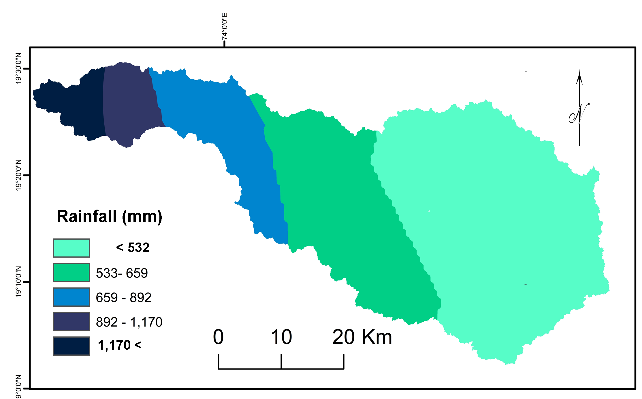
3.2.4 Rainfall
Rainfall plays a significant role in life system and top soil erosion (Petkovsek and Mikos, 2004) and varies for amount, intensity and distribution. The region receives rainfall during the Southwest monsoon season (June to October) and show high variation from 467 mm at Eastern part to 1505mm at West (World climate data, mean rainfall 1970 to 2000) (Figure 26). Eastern part of the basin is known as ‘rain shadow’ zone of Sahyadri Ghats. It is severe drought prone area in the state of Maharashtra (India). Higher variations in rainfall distribution can be useful for periodization of sub-watersheds in the basin.
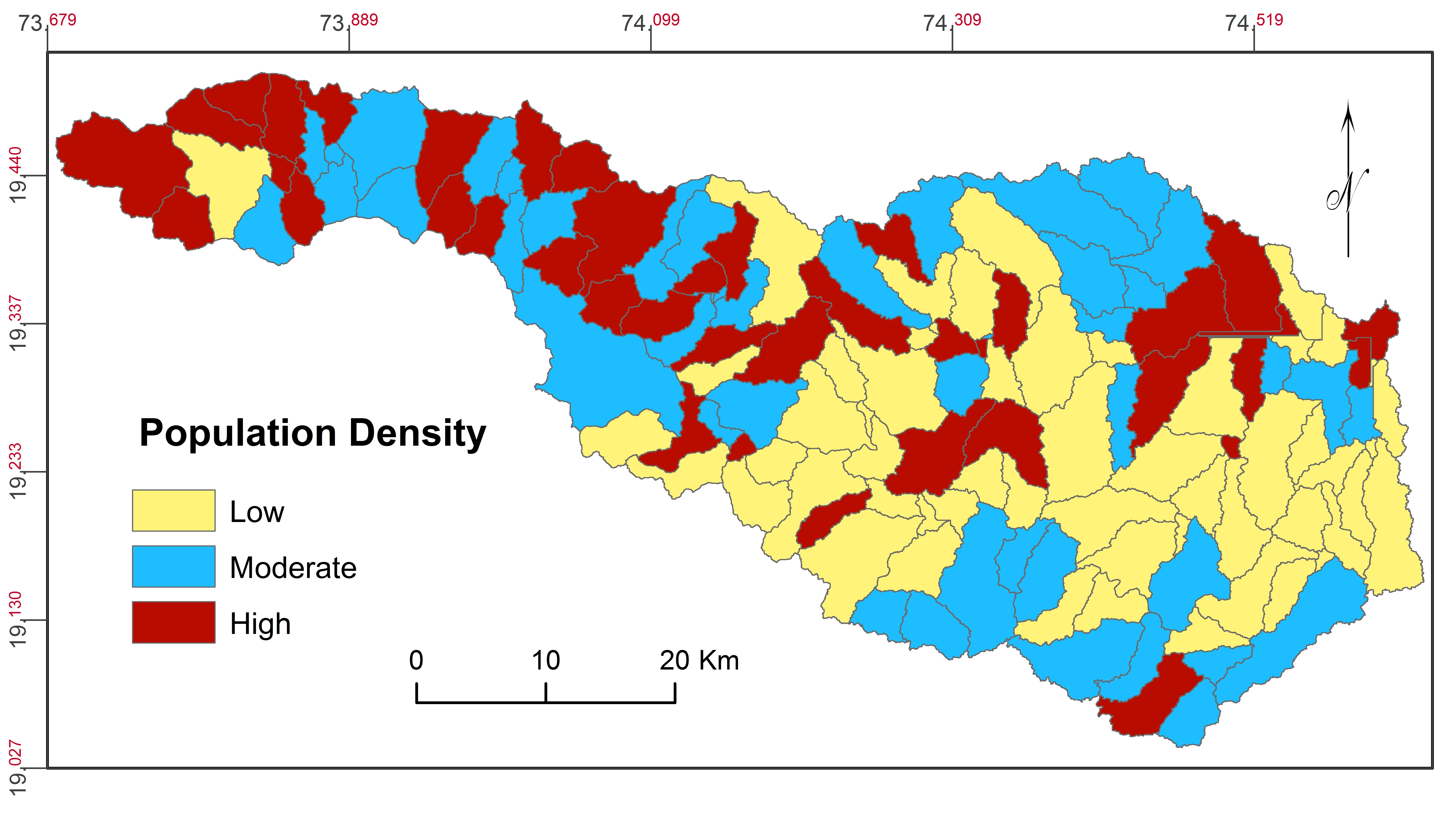
3.2.5 Population Density
The growth of global population needs effective management of decreasing pressure on natural resources available for agricultural (Mishra and Nagarajan, 2010; Gumma et al., 2014). About 70% of population of India depends on agriculture, directly or indirectly (Rao et al., 2010). Total population of the basin was 254901 in 2001 and increased to 289211 in 2011 (Census, 2011). Majority of population is belongs to tribal community living in about 50% villages (165) at Western part of the basin. This is hilly region and people facing many problems like lack of educational, transportation, medical facilities, etc. It is notable that 39 villages show decreasing trends of population from 2001 to 2011 due to outmigration. Further, Eastern part is drought-prone and people are migrating for their sustenance, occasionally. Therefore, population distribution (Figure 27) is significant criteria for analysis of prioritization of watersheds for natural resource management and planning.
3.3 Analytic Hierarchy Process for Watershed Prioritization
Analytic Hierarchy Process is processed for prioritization of sub-watersheds as: (1) determination of ranks, (2) pairwise comparison matrixes, (3) normalization of pairwise comparison matrix, (4) calculation of weights and influence, (5) normalization of sub-watershed wise influences, and (6) prioritization of sub-watersheds.
3.3.1 Determination of Ranks
Statistical approach was used for assigning the ranks for 25 criterion using weighted analyses. We have used correlation techniques for robust ranking of parameters for water prioritization of watersheds using AHP based influence approach (Gaikwad and Bhagat, 2017). This was used by Zolekar and Bhagat (2015) for land suitability analysis using AHP based weighted overlay technique. Calculated significant correlation coefficients of the criteria with criterion in the group were summed up for ranking the selected criterion (Aher et al., 2014). Pearson’s correlation technique (Yin et al., 2012) (Table 2) was used for correlation analysis and 1 to 24 ranks were assigned (Table 2) (Ranjan, 2013; Zolekar and Bhagat, 2015; Gaikwad and Bhagat, 2017). Maximum sum of corrections was estimated for texture ratio (25.94), drainage texture, (12.97), total streams (8.65), stream length (6.49), ruggedness number (5.19), drainage density (4.32) and therefore 1 to 6 ranks given, respectively (Table 3). Ranks, 7 to 13 were given to criterion estimated moderate values for basin length, area, infiltration number, perimeter, bifurcation ratio, stream frequency and rainfall whereas population density, slope, soil, relief ratio, elongation ratio, circulatory ratio, form factor, shape factor, mean stream length, compactness ratio, stream length ratio and geology were ranked least.
Table 3. Correlations
| |
Area
|
\(P\)
|
\(D_d\)
|
\(T\)
|
\(L_b\)
|
\(R_c\)
|
\(C_C\)
|
\(R_f\)
|
\(R_e\)
|
\(L_u\)
|
\(N_u\)
|
\(F_s\)
|
\(L_{sm}\)
|
RL
|
\(R_b\)
|
\(R_t\)
|
\(B_s\)
|
\(I_f\)
|
\(R_{h1}\)
|
\(R_n\)
|
Geology
|
Slope
|
Soil
|
Rainfall
|
PD
|
|
Area
|
1.00
|
|
|
|
|
|
|
|
|
|
|
|
|
|
|
|
|
|
|
|
|
|
|
|
|
|
\(P\)
|
0.91
|
1.00
|
|
|
|
|
|
|
|
|
|
|
|
|
|
|
|
|
|
|
|
|
|
|
|
|
\(D_d\)
|
0.15
|
0.13
|
1.00
|
|
|
|
|
|
|
|
|
|
|
|
|
|
|
|
|
|
|
|
|
|
|
|
\(T\)
|
0.49
|
0.29
|
0.49
|
1.00
|
|
|
|
|
|
|
|
|
|
|
|
|
|
|
|
|
|
|
|
|
|
|
\(L_b\)
|
0.82
|
0.87
|
0.21
|
0.37
|
1.00
|
|
|
|
|
|
|
|
|
|
|
|
|
|
|
|
|
|
|
|
|
|
\(R_c\)
|
0.04
|
-0.19
|
-0.04
|
0.45
|
-0.05
|
1.00
|
|
|
|
|
|
|
|
|
|
|
|
|
|
|
|
|
|
|
|
|
\(C_C\)
|
0.06
|
0.35
|
-0.16
|
-0.44
|
0.23
|
-0.46
|
1.00
|
|
|
|
|
|
|
|
|
|
|
|
|
|
|
|
|
|
|
|
\(R_f\)
|
0.02
|
0.02
|
-0.11
|
-0.02
|
-0.26
|
0.02
|
-0.02
|
1.00
|
|
|
|
|
|
|
|
|
|
|
|
|
|
|
|
|
|
|
\(R_e\)
|
0.00
|
-0.05
|
-0.15
|
0.00
|
-0.39
|
0.07
|
-0.14
|
0.95
|
1.00
|
|
|
|
|
|
|
|
|
|
|
|
|
|
|
|
|
|
\(L_u\)
|
0.90
|
0.79
|
0.48
|
0.61
|
0.75
|
0.00
|
0.00
|
-0.02
|
-0.05
|
1.00
|
|
|
|
|
|
|
|
|
|
|
|
|
|
|
|
|
\(N_u\)
|
0.85
|
0.73
|
0.40
|
0.74
|
0.70
|
-0.04
|
-0.02
|
-0.02
|
-0.05
|
0.91
|
1.00
|
|
|
|
|
|
|
|
|
|
|
|
|
|
|
|
\(F_s\)
|
-0.01
|
-0.05
|
0.55
|
0.63
|
0.02
|
-0.10
|
-0.19
|
-0.08
|
-0.09
|
0.19
|
0.44
|
1.00
|
|
|
|
|
|
|
|
|
|
|
|
|
|
|
\(L_{sm}\)
|
0.09
|
0.09
|
0.28
|
-0.15
|
0.09
|
0.17
|
0.04
|
-0.10
|
-0.11
|
0.14
|
-0.13
|
-0.47
|
1.00
|
|
|
|
|
|
|
|
|
|
|
|
|
|
RL
|
-0.04
|
-0.05
|
0.12
|
0.00
|
-0.01
|
0.01
|
-0.16
|
-0.08
|
-0.10
|
-0.03
|
-0.03
|
0.05
|
0.17
|
1.00
|
|
|
|
|
|
|
|
|
|
|
|
|
\(R_b\)
|
0.45
|
0.54
|
0.37
|
0.45
|
0.55
|
0.02
|
-0.21
|
-0.04
|
-0.07
|
0.44
|
0.44
|
0.24
|
0.03
|
0.20
|
1.00
|
|
|
|
|
|
|
|
|
|
|
|
\(R_t\)
|
0.49
|
0.29
|
0.49
|
1.00
|
0.37
|
0.45
|
-0.44
|
-0.02
|
0.00
|
0.61
|
0.74
|
0.63
|
-0.15
|
0.00
|
0.45
|
1.00
|
|
|
|
|
|
|
|
|
|
|
\(B_s\)
|
-0.03
|
0.12
|
-0.01
|
-0.16
|
0.41
|
-0.12
|
0.49
|
-0.29
|
-0.51
|
-0.02
|
-0.03
|
-0.04
|
0.00
|
0.10
|
-0.02
|
-0.16
|
1.00
|
|
|
|
|
|
|
|
|
|
\(I_f\)
|
0.03
|
0.00
|
0.81
|
0.63
|
0.06
|
-0.07
|
-0.20
|
-0.07
|
-0.07
|
0.32
|
0.44
|
0.89
|
-0.19
|
0.04
|
0.29
|
0.63
|
-0.06
|
1.00
|
|
|
|
|
|
|
|
|
\(R_{h1}\)
|
-0.21
|
-0.31
|
0.15
|
0.06
|
-0.39
|
0.00
|
-0.05
|
0.28
|
0.33
|
-0.07
|
-0.05
|
0.15
|
-0.10
|
-0.22
|
-0.41
|
0.06
|
-0.32
|
0.19
|
1.00
|
|
|
|
|
|
|
|
\(R_n\)
|
0.22
|
0.15
|
0.76
|
0.49
|
0.20
|
-0.03
|
-0.20
|
-0.06
|
-0.06
|
0.49
|
0.43
|
0.41
|
0.12
|
-0.01
|
0.27
|
0.49
|
-0.06
|
0.64
|
0.43
|
1.00
|
|
|
|
|
|
|
Geology
|
0.00
|
0.00
|
-0.05
|
-0.01
|
0.01
|
-0.01
|
-0.03
|
-0.01
|
-0.02
|
-0.03
|
-0.02
|
-0.03
|
-0.03
|
0.00
|
0.03
|
-0.01
|
0.00
|
-0.05
|
-0.02
|
-0.03
|
1.00
|
|
|
|
|
|
Slope
|
0.36
|
0.28
|
0.17
|
0.32
|
0.26
|
-0.03
|
-0.08
|
-0.04
|
-0.04
|
0.40
|
0.42
|
0.14
|
-0.01
|
-0.01
|
0.19
|
0.32
|
-0.06
|
0.14
|
0.03
|
0.26
|
-0.02
|
1.00
|
|
|
|
|
Soil
|
0.14
|
0.12
|
0.15
|
0.19
|
0.11
|
-0.05
|
-0.04
|
0.13
|
0.09
|
0.18
|
0.23
|
0.18
|
-0.12
|
0.07
|
0.12
|
0.19
|
-0.04
|
0.19
|
0.03
|
0.14
|
0.01
|
0.00
|
1.00
|
|
|
|
Rainfall
|
0.02
|
-0.12
|
0.47
|
0.41
|
-0.05
|
0.01
|
-0.33
|
-0.05
|
0.00
|
0.24
|
0.28
|
0.41
|
-0.05
|
0.11
|
0.08
|
0.41
|
-0.15
|
0.51
|
0.52
|
0.75
|
0.04
|
0.19
|
0.11
|
1.00
|
|
|
PD*
|
0.09
|
0.00
|
0.28
|
0.30
|
0.12
|
0.16
|
-0.24
|
-0.09
|
-0.08
|
0.21
|
0.18
|
0.17
|
0.04
|
-0.01
|
0.13
|
0.30
|
0.02
|
0.25
|
0.23
|
0.39
|
0.03
|
0.15
|
0.09
|
0.36
|
1.00
|
*PD = population density
Table 4. Ranks
|
Criterion
|
\(T\)
|
\(R_t\)
|
\(N_u\)
|
\(L_u\)
|
\(R_n\)
|
\(D_d\)
|
\(L_b\)
|
Area
|
\(I_f\)
|
\(P\)
|
\(R_b\)
|
\(F_s\)
|
Rainfall
|
PD
|
Slope
|
Soil
|
\(R_{h1}\)
|
\(R_e\)
|
\(R_c\)
|
\(R_f\)
|
\(B_s\)
|
\(L_{sm}\)
|
\(C_C\)
|
RL
|
Geology
|
|
Sum of significant coefficient of correlation
|
9.99
|
9.99
|
9.97
|
9.75
|
8.65
|
8.46
|
8.26
|
8.10
|
7.99
|
7.70
|
7.21
|
7.10
|
6.84
|
5.76
|
5.68
|
4.44
|
4.40
|
3.45
|
3.43
|
3.36
|
3.26
|
3.14
|
3.13
|
2.82
|
2.00
|
|
Ranks
|
1
|
2
|
3
|
4
|
5
|
6
|
7
|
8
|
9
|
10
|
11
|
12
|
13
|
14
|
15
|
16
|
17
|
18
|
19
|
20
|
21
|
22
|
23
|
24
|
25
|
3.3.2 Pairwise Comparison Matrix (PCM)
Multiple criteria decision-making and pairwise comparison matrix are useful for prioritization of sub-watersheds (Sepehr et al., 2017; Ghanbarpour and Hipel, 2011; Rekha et al., 2011; Feizizadeh et al., 2014). The influences of criterion were estimated based weights given in pairwise comparison matrix (Zolekar and Bhagat, 2015). Emamgholi et al. (2007) and Ranjan (2013) have used PCM to understand the relationship between the criterion and surface erosion for conservation of natural resources in the watershed.
The values of the criterion in matrix were divided by total of the column to calculate cell values (Table 4).
3.3.3 Weights and Influences
Weights of criterion were estimated based on weights and influences calculated in normalized pairwise comparison matrix after Gaikwad and Bhagat (2017) (Table 4). Influences of criterion were estimated by calculating the cell values (%) in PCM (Gaikwad and Bhagat, 2017) (Equation 1):
\(C_i = \frac {W_c}{W_s} \times 100\) (1)
\(C_i\) = Normalized influence of criterion based on AHP.
\(W_c\) = Estimated weights of criterion.
\(W_s\) = Sum of estimated weights for all criterions.
\(C_i\) = Indicate the share of criterion in total influence (100%) of criterion which can be distributed within the criterion according to estimated weights (Gaikwad and Bhagat, 2017).
Table 5. Weights and influence
| |
\(T\)
|
\(R_t\)
|
\(N_u\)
|
\(L_u\)
|
\(R_n\)
|
\(D_d\)
|
\(L_b\)
|
Area
|
\(I_f\)
|
P
|
\(R_b\)
|
\(F_s\)
|
Rainfall
|
PD
|
Slope
|
Soil
|
\(R_{h1}\)
|
\(R_e\)
|
\(R_c\)
|
\(R_f\)
|
\(B_s\)
|
\(L_{sm}\)
|
\(C_C\)
|
RL
|
Geology
|
Sum
|
Weights
|
Influence (%)
|
|
\(T\)
|
0.26
|
0.26
|
0.26
|
0.26
|
0.26
|
0.26
|
0.26
|
0.26
|
0.26
|
0.26
|
0.26
|
0.26
|
0.26
|
0.26
|
0.26
|
0.26
|
0.26
|
0.26
|
0.26
|
0.26
|
0.26
|
0.26
|
0.26
|
0.26
|
0.26
|
6.75
|
0.26
|
25.94
|
|
\(R_t\)
|
0.13
|
0.13
|
0.13
|
0.13
|
0.13
|
0.13
|
0.13
|
0.13
|
0.13
|
0.13
|
0.13
|
0.13
|
0.13
|
0.13
|
0.13
|
0.13
|
0.13
|
0.13
|
0.13
|
0.13
|
0.13
|
0.13
|
0.13
|
0.13
|
0.13
|
3.37
|
0.13
|
12.97
|
|
\(N_u\)
|
0.09
|
0.09
|
0.09
|
0.09
|
0.09
|
0.09
|
0.09
|
0.09
|
0.09
|
0.09
|
0.09
|
0.09
|
0.09
|
0.09
|
0.09
|
0.09
|
0.09
|
0.09
|
0.09
|
0.09
|
0.09
|
0.09
|
0.09
|
0.09
|
0.09
|
2.25
|
0.09
|
8.65
|
|
\(L_u\)
|
0.06
|
0.06
|
0.06
|
0.06
|
0.06
|
0.06
|
0.06
|
0.06
|
0.06
|
0.06
|
0.06
|
0.06
|
0.06
|
0.06
|
0.06
|
0.06
|
0.06
|
0.06
|
0.06
|
0.06
|
0.06
|
0.06
|
0.06
|
0.06
|
0.06
|
1.69
|
0.06
|
6.49
|
|
\(R_n\)
|
0.05
|
0.05
|
0.05
|
0.05
|
0.05
|
0.05
|
0.05
|
0.05
|
0.05
|
0.05
|
0.05
|
0.05
|
0.05
|
0.05
|
0.05
|
0.05
|
0.05
|
0.05
|
0.05
|
0.05
|
0.05
|
0.05
|
0.05
|
0.05
|
0.05
|
1.35
|
0.05
|
5.19
|
|
\(D_d\)
|
0.04
|
0.04
|
0.04
|
0.04
|
0.04
|
0.04
|
0.04
|
0.04
|
0.04
|
0.04
|
0.04
|
0.04
|
0.04
|
0.04
|
0.04
|
0.04
|
0.04
|
0.04
|
0.04
|
0.04
|
0.04
|
0.04
|
0.04
|
0.04
|
0.04
|
1.12
|
0.04
|
4.32
|
|
\(L_b\)
|
0.04
|
0.04
|
0.04
|
0.04
|
0.04
|
0.04
|
0.04
|
0.04
|
0.04
|
0.04
|
0.04
|
0.04
|
0.04
|
0.04
|
0.04
|
0.04
|
0.04
|
0.04
|
0.04
|
0.04
|
0.04
|
0.04
|
0.04
|
0.04
|
0.04
|
0.96
|
0.04
|
3.71
|
|
Area
|
0.03
|
0.03
|
0.03
|
0.03
|
0.03
|
0.03
|
0.03
|
0.03
|
0.03
|
0.03
|
0.03
|
0.03
|
0.03
|
0.03
|
0.03
|
0.03
|
0.03
|
0.03
|
0.03
|
0.03
|
0.03
|
0.03
|
0.03
|
0.03
|
0.03
|
0.84
|
0.03
|
3.24
|
|
\(I_f\)
|
0.03
|
0.03
|
0.03
|
0.03
|
0.03
|
0.03
|
0.03
|
0.03
|
0.03
|
0.03
|
0.03
|
0.03
|
0.03
|
0.03
|
0.03
|
0.03
|
0.03
|
0.03
|
0.03
|
0.03
|
0.03
|
0.03
|
0.03
|
0.03
|
0.03
|
0.75
|
0.03
|
2.88
|
|
P
|
0.03
|
0.03
|
0.03
|
0.03
|
0.03
|
0.03
|
0.03
|
0.03
|
0.03
|
0.03
|
0.03
|
0.03
|
0.03
|
0.03
|
0.03
|
0.03
|
0.03
|
0.03
|
0.03
|
0.03
|
0.03
|
0.03
|
0.03
|
0.03
|
0.03
|
0.67
|
0.03
|
2.59
|
|
\(R_b\)
|
0.02
|
0.02
|
0.02
|
0.02
|
0.02
|
0.02
|
0.02
|
0.02
|
0.02
|
0.02
|
0.02
|
0.02
|
0.02
|
0.02
|
0.02
|
0.02
|
0.02
|
0.02
|
0.02
|
0.02
|
0.02
|
0.02
|
0.02
|
0.02
|
0.02
|
0.61
|
0.02
|
2.36
|
|
\(F_s\)
|
0.02
|
0.02
|
0.02
|
0.02
|
0.02
|
0.02
|
0.02
|
0.02
|
0.02
|
0.02
|
0.02
|
0.02
|
0.02
|
0.02
|
0.02
|
0.02
|
0.02
|
0.02
|
0.02
|
0.02
|
0.02
|
0.02
|
0.02
|
0.02
|
0.02
|
0.56
|
0.02
|
2.16
|
|
Rainfall
|
0.02
|
0.02
|
0.02
|
0.02
|
0.02
|
0.02
|
0.02
|
0.02
|
0.02
|
0.02
|
0.02
|
0.02
|
0.02
|
0.02
|
0.02
|
0.02
|
0.02
|
0.02
|
0.02
|
0.02
|
0.02
|
0.02
|
0.02
|
0.02
|
0.02
|
0.52
|
0.02
|
2.00
|
|
PD
|
0.02
|
0.02
|
0.02
|
0.02
|
0.02
|
0.02
|
0.02
|
0.02
|
0.02
|
0.02
|
0.02
|
0.02
|
0.02
|
0.02
|
0.02
|
0.02
|
0.02
|
0.02
|
0.02
|
0.02
|
0.02
|
0.02
|
0.02
|
0.02
|
0.02
|
0.48
|
0.02
|
1.85
|
|
Slope
|
0.02
|
0.02
|
0.02
|
0.02
|
0.02
|
0.02
|
0.02
|
0.02
|
0.02
|
0.02
|
0.02
|
0.02
|
0.02
|
0.02
|
0.02
|
0.02
|
0.02
|
0.02
|
0.02
|
0.02
|
0.02
|
0.02
|
0.02
|
0.02
|
0.02
|
0.45
|
0.02
|
1.73
|
|
Soil
|
0.02
|
0.02
|
0.02
|
0.02
|
0.02
|
0.02
|
0.02
|
0.02
|
0.02
|
0.02
|
0.02
|
0.02
|
0.02
|
0.02
|
0.02
|
0.02
|
0.02
|
0.02
|
0.02
|
0.02
|
0.02
|
0.02
|
0.02
|
0.02
|
0.02
|
0.42
|
0.02
|
1.62
|
|
\(R_{h1}\)
|
0.02
|
0.02
|
0.02
|
0.02
|
0.02
|
0.02
|
0.02
|
0.02
|
0.02
|
0.02
|
0.02
|
0.02
|
0.02
|
0.02
|
0.02
|
0.02
|
0.02
|
0.02
|
0.02
|
0.02
|
0.02
|
0.02
|
0.02
|
0.02
|
0.02
|
0.40
|
0.02
|
1.53
|
|
\(R_e\)
|
0.01
|
0.01
|
0.01
|
0.01
|
0.01
|
0.01
|
0.01
|
0.01
|
0.01
|
0.01
|
0.01
|
0.01
|
0.01
|
0.01
|
0.01
|
0.01
|
0.01
|
0.01
|
0.01
|
0.01
|
0.01
|
0.01
|
0.01
|
0.01
|
0.01
|
0.37
|
0.01
|
1.44
|
|
\(R_f\)
|
0.01
|
0.01
|
0.01
|
0.01
|
0.01
|
0.01
|
0.01
|
0.01
|
0.01
|
0.01
|
0.01
|
0.01
|
0.01
|
0.01
|
0.01
|
0.01
|
0.01
|
0.01
|
0.01
|
0.01
|
0.01
|
0.01
|
0.01
|
0.01
|
0.01
|
0.36
|
0.01
|
1.37
|
|
\(B_s\)
|
0.01
|
0.01
|
0.01
|
0.01
|
0.01
|
0.01
|
0.01
|
0.01
|
0.01
|
0.01
|
0.01
|
0.01
|
0.01
|
0.01
|
0.01
|
0.01
|
0.01
|
0.01
|
0.01
|
0.01
|
0.01
|
0.01
|
0.01
|
0.01
|
0.01
|
0.34
|
0.01
|
1.30
|
|
\(L_{sm}\)
|
0.01
|
0.01
|
0.01
|
0.01
|
0.01
|
0.01
|
0.01
|
0.01
|
0.01
|
0.01
|
0.01
|
0.01
|
0.01
|
0.01
|
0.01
|
0.01
|
0.01
|
0.01
|
0.01
|
0.01
|
0.01
|
0.01
|
0.01
|
0.01
|
0.01
|
0.32
|
0.01
|
1.24
|
|
\(C_C\)
|
0.01
|
0.01
|
0.01
|
0.01
|
0.01
|
0.01
|
0.01
|
0.01
|
0.01
|
0.01
|
0.01
|
0.01
|
0.01
|
0.01
|
0.01
|
0.01
|
0.01
|
0.01
|
0.01
|
0.01
|
0.01
|
0.01
|
0.01
|
0.01
|
0.01
|
0.29
|
0.01
|
1.13
|
|
\(C_C\)
|
0.01
|
0.01
|
0.01
|
0.01
|
0.01
|
0.01
|
0.01
|
0.01
|
0.01
|
0.01
|
0.01
|
0.01
|
0.01
|
0.01
|
0.01
|
0.01
|
0.01
|
0.01
|
0.01
|
0.01
|
0.01
|
0.01
|
0.01
|
0.01
|
0.01
|
0.28
|
0.01
|
1.08
|
|
RL
|
0.01
|
0.01
|
0.01
|
0.01
|
0.01
|
0.01
|
0.01
|
0.01
|
0.01
|
0.01
|
0.01
|
0.01
|
0.01
|
0.01
|
0.01
|
0.01
|
0.01
|
0.01
|
0.01
|
0.01
|
0.01
|
0.01
|
0.01
|
0.01
|
0.01
|
0.27
|
0.01
|
1.04
|
|
Geology
|
0.01
|
0.01
|
0.01
|
0.01
|
0.01
|
0.01
|
0.01
|
0.01
|
0.01
|
0.01
|
0.01
|
0.01
|
0.01
|
0.01
|
0.01
|
0.01
|
0.01
|
0.01
|
0.01
|
0.01
|
0.01
|
0.01
|
0.01
|
0.01
|
0.01
|
0.26
|
0.01
|
1.00
|
3.3.4 Watershed Based Normalized Influence of Criterion
The influences of criterion interpret the share of individual criteria in formation of watershed characteristics (100%) and vary according to sub-watersheds (Silva et al., 2007; Gaikwad and Bhagat, 2017). Here, sub-watershed wise influences of criterion were normalized (equation 2) (Gaikwad and Bhagat, 2017).
\(NI_w = \frac {C_w}{C_s} \times C_i\) (2)
\(NI_w\) = Sub-watershed wise normalized influence.
\(C_w\) = Cell value of criterion for the watershed
\(C_s\) = Sum of cell values of criterion.
\(C_i\) = Estimated influence of criterion based on AHP.
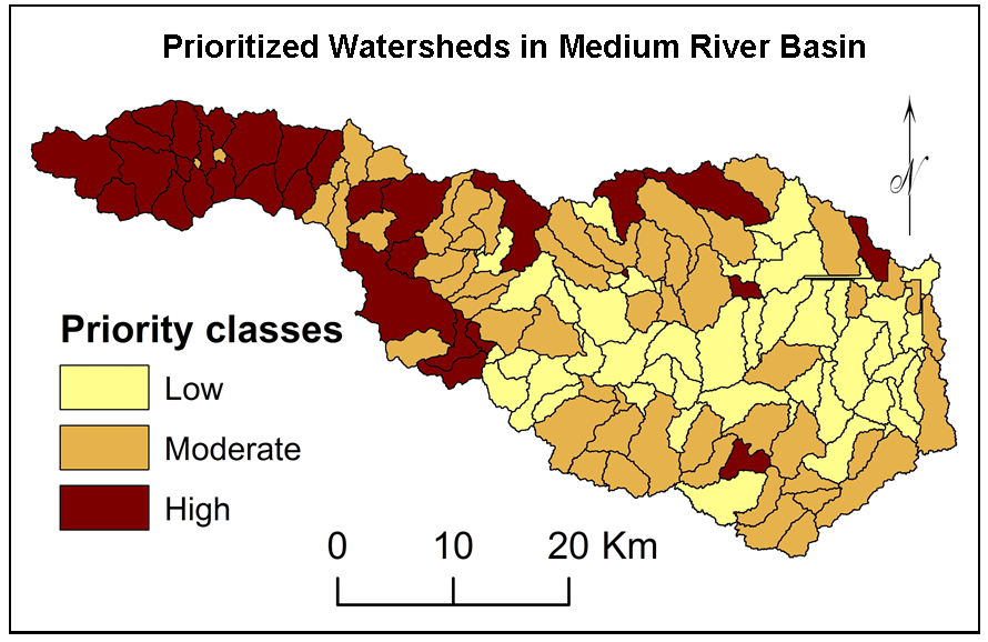
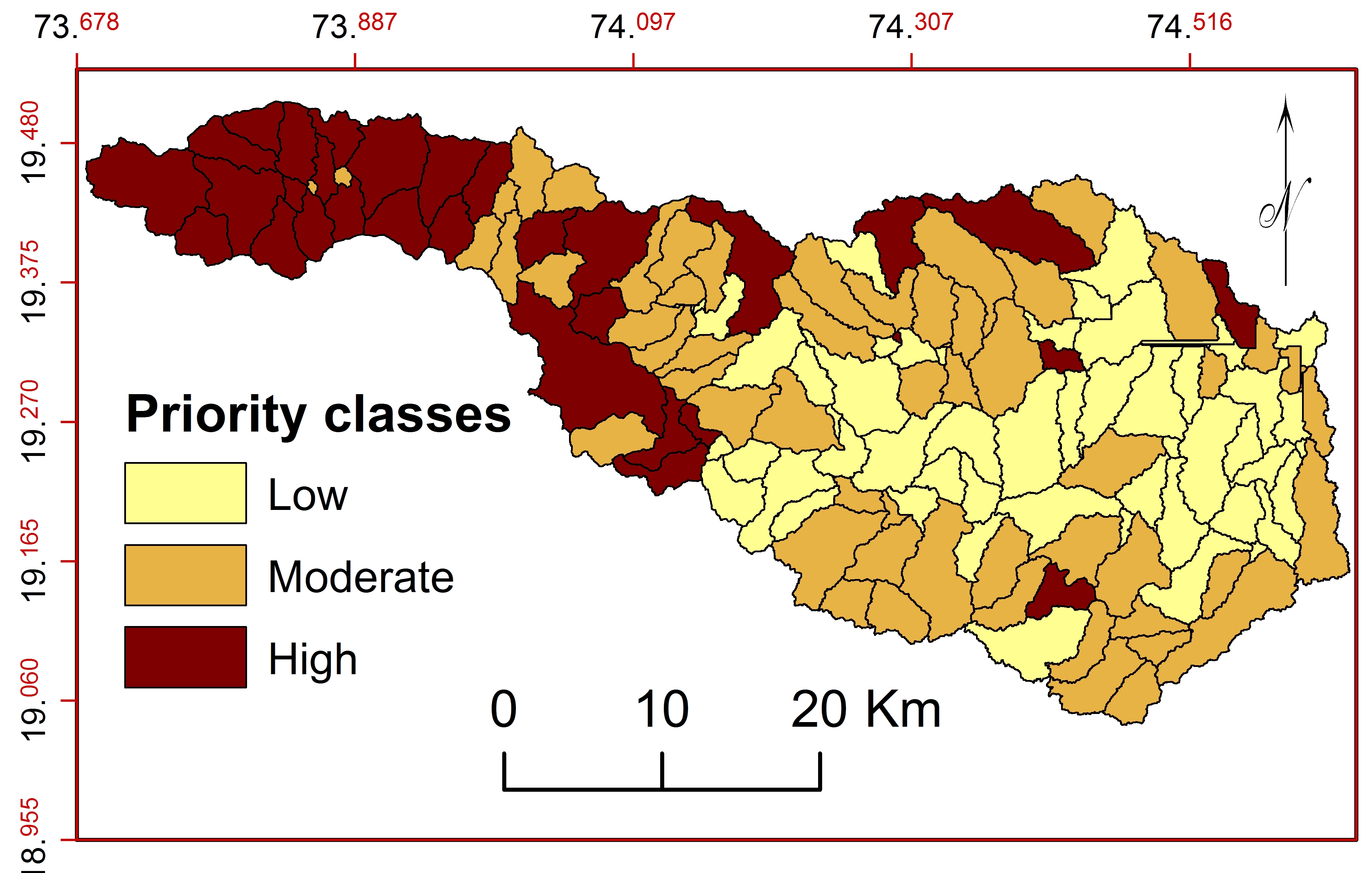
3.3.5 Weighted prioritization
Spatial variations in geology, morphometric parameters, soils, rainfall and population densities were used for watershed prioritization. These parameters can be useful to decide the level of soil and water degradation and for prioritization of sub-watersheds (Aher et al., 2014) using normalized PCM (Ghanbarpour and Hipel, 2011), calculated influences for criterion and sub-watershed wise normalized influences (Gaikwad and Bhagat, 2017).
\(P_w=\displaystyle\sum_{i=1}^{n} NI_w\) (3)
\(P_w\) = Periodization of watershed
\(NI_w\) = Sub-watershed wise normalized influence.
\(n\) = Number of criterion
\(i\) = Criterion


 ,
Vijay Bhagat 2
,
Vijay Bhagat 2