Keywords

Groundwater , Groundwater Potential Zones , AHP , Remote Sensing , GIS , Exploration

1 . INTRODUCTION

Groundwater is a prime source for drinking and irrigation, anyway this fundamental asset is at risk for contamination because of human tendency to devour a greater amount of the groundwater (Shekhar and Pandey, 2015; Murthy et al., 2003). The large urbanization has influencing the groundwater quality due to over- and misuse of assets and ill-advised waste transfer rehearses. Water quality is controlled by the solutes and gases broke up in the water, just as the issue suspended in and gliding on the water (Raju et al., 2017). It results of the regular physical and chemical condition of water just as any adjustments that may have happened as an outcome of human action. Groundwater varies  spatially and seasonally with the profundity of water table (Kumar et al., 2014, Kumar et al. 2015). Therefore, many groundwater studies show importance of groundwater evaluation for quantification (Pathak, 2017).

Remote Sensing (RS) and Geographic Information System (GIS) are extensively used for the exploration and managing of different natural resources i.e. groundwater, minerals, etc. In the recent years, many authors were effectively identified the water table elevation using geospatial techniques (Rajasekhar et al., 2018; Siddi et al. , 2018). RS method gives leeway of approaching vast inclusion, even in in-accessible areas. It is fast and cost effective in delivering profitable information on geology, lineament density, lineaments, slope, geomorphology, drainage density, soils, rainfall and land use / land cover (LULC) (Basha et al., 2018; Raju et al., 2018). GWPZ map has been categorized as poor, moderate, good, and very good dependent on the groundwater accessibility in study region.

In semi-arid areas (Andhra Pradesh: Anantapur, Kadapa) covered by hard rock terrain, groundwater can be identified in shallow aquifers flooring the main valleys and fractured zones in the bedrocks (Ankidawa and Seli, 2018; Mallick et al., 2014; Pathak, 2017; Taylor et al., 2013).

The water-bearing formations in the intermountain basin store broad proportions of non-inexhaustible that acknowledged to have been recharged in the midst of past wet climatic periods. The shallow-fracture zone aquifers have sustainable water that is recharged by direct infiltration from monsoonal rainfall (Kadam, et al., 2017; Mundalik et al., 2018; Waikar, 2015; Singhai et al., 2017). Groundwater aggregations can be found in crystalline rocks inside much distorted zones, for example, shear and fault zones.  It is difficult to choose the system of the fracture structure or to predict whether groundwater is presumably going to happen in the fractures. As a rule, drilling is the most ideal approach to avow the proximity of groundwater (Amer et al., 2013; Shrestha, 2018).

In the present years the significance of coupling geospatial methods in GWP evaluation examines was acknowledged by numerous scientists to outline and differentiate the groundwater assets using geospatial information depends on a circuitous examination of some specifically perceptible surface landscapes like geomorphology, geology, slope, LULC and hydrologic characteristics (Basha et al., 2017).

With the proficiencies of the geospatial information, various databases can be incorporated to create conceptual model for identification and estimation of GWPZs. An endeavor has been made to depict the GWPZs in Kadapa of Andhra Pradesh, India. With this intent Veerapanayani Palli mandal is choose with the objectives to: (1) understand the properties of different thematic layer on groundwater, (2) demarcated the groundwater potential sites, and (3) determine the sites with field overview to measure precision of technique adopted for the study.

2 . STUDY AREA

The study area shields an area of 293.64 km² and lies between the 14º 28ʹ 40" to 14º 31ʹ 36"N latitudes and 78º 22ʹ 58" to 78º 35ʹ 8" E longitudes (Figure 1). The study area comprised of different lithological units such as shale tuffs, vempalli dolomites, volcanic flows and quartzite. Annual average rainfall is 464.5mm with rainy days experience of sub-tropical climate. The area consists of various geomorphological features such as denudational origin-low dissected hills and valleys, structural origin with low dissected hills, pediment-pediplain complex with water bodies. The accessible water is adequate amid the early piece of the winter season; later, the water table decays quickly, and by summer, a large number of the shallow wells tapping the upper unconfined aquifers either ended up being dry or don’t adequately meet the essential. Along these lines, in spite of the way that there is a lot of surface water, there is an exceptional insufficiency of water in summer. Thus, there is a need to recognize zones where area explicit artificial recharge techniques can be grasped to extend water supply.

Figure 1. Study area: Veerapanayani Palle

3 . METHODOLOGY

3.1 Preparation of Thematic Maps

GIS is a primary tool to carry out preparation of various thematic maps of the study area. Thematic maps pertaining to geology, drainage density, lineament density, and geomorphology were done from satellite imageries with Survey of India (SOI) topographic maps (Marhaento, 2018; Mukherjee and Kumar, 2018; Pathak, 2017; Rahmati et al., 2015). Slope map was prepared from Cartosat Digital Elevation Model (DEM) with the ArcGIS environment. Soil map was prepared using National Bureau of Soil Survey and Land Use Planning (NBSSLUP), Nagpur (Agarwal et al., 2013). Rainfall interpolation map was prepared using collateral data obtained from Chief planning officer at district collector of the study region. These all the thematic layers are integrated into an ArcGIS environment, which would help the identification of GWPZ. The methodology adopted for the present study is shown in Figure 2.

Figure 2. Methodology

3.2 Assignment and Normalization of Weights

AHP for choice building in which an issue is separated into different parameters, assembling them in a various leveled structure, settling on choices on the overall significance of sets of parts and mixing the results (Saaty, 1999).

Every thematic map has more than five classes, which demonstrates the associations between these interrelated classes are too much excessively intricate. Thus, the relationship between these eight thematic layers has been construed using the distinctive classes has been recognized using AHP (Kadam et al., 2017) (Figure 2). The framework for deciding the weights to the thematic maps and their looking at classes using AHP independently incorporates the going with advances (Jhariya, 2016)

3.3 Pairwise Comparison Matrices

The relative significance levels are resolved with Saaty's 1-9 scale (Table 1), where a score of 1 denotes to even with significance between the 2 layers, and a score of 9 shows the extraordinary significance of 1 layer contrasted with the additional one (Saaty, 1980).

Table 2 demonstrates a matrix for contrasting the classes all together with accomplishing the need. A pairwise comparison matrix is inferred utilizing Saaty's 9 points significance scale dependent on thematic maps utilized for an outline of GWP.

The AHP catches the possibility of a vulnerability in decisions through the main eigenvalue and the consistency index (Saaty, 2004; Agarwal et al., 2013; Machiwal et al., 2011; Mallick et al., 2014; Rahmati et al., 2015). Saaty gaves a proportion of consistency, called Consistency Index (CI) as deviation or level of consistency utilizing the accompanying condition (Equation (1)):

\(CI = {\lambda max-n \over n-1}\)          (1)

where, λ max is the largest eigenvalue of the pair-wise comparison matrix and n is the number of classes.

Consistency Ratio (CR) is a measure of consistency of pairwise comparison matrix (Equation (2)):

\(CR = {CI \over RI}\)                (2)

where, RI is the Ratio Index. The value of RI for different n values is given in Table 3.

3.4 Verification of the Groundwater Potential Zones

GWPZ identified in the study was confirmed based on accessible well yield information from Groundwater Department, Kadapa, Andhra Pradesh. The well yield focuses were overlaid on the final GWPZ map to cross-check the precision of the present work in the different GWPZs.

4 . RESULTS AND DISCUSSION

A precise methodology for groundwater asset assessment of any region requires the comprehensive study of different parameters like geology, geomorphology, LULC, lineament density, drainage density, soils, slope and rainfall (Sikdar et al., 2004). So as to delineate GWPZs in the study area, distinctive thematic layers were setup from RS information, topographic maps and land maps related to the collateral maps and field overview. The details of the thematic maps produced from the satellite and field information, together with the groundwater possibilities:

4.1 Geology

Geological map was prepared by digitizing each lithologic unit in ArcGIS 10.4 software using secured by with a major part as shale tuff and some parts with dolomites (Figure 3). These shale rocks are crossed by means of volcanic flows as dolerite dykes. In the northern part of the area, a secluded patch of quartzite’s are formed. According to the pairwise comparison matrix of geology map was resulted on the significance of aquifer type to conserve the groundwater. The study region was classified in various lithology based upon their properties on aquifer type having higher vemaplli dolomites with moderate storage in shale tuff with quarzites and poor storage towards volcanic flows.

Figure 3. Rocks

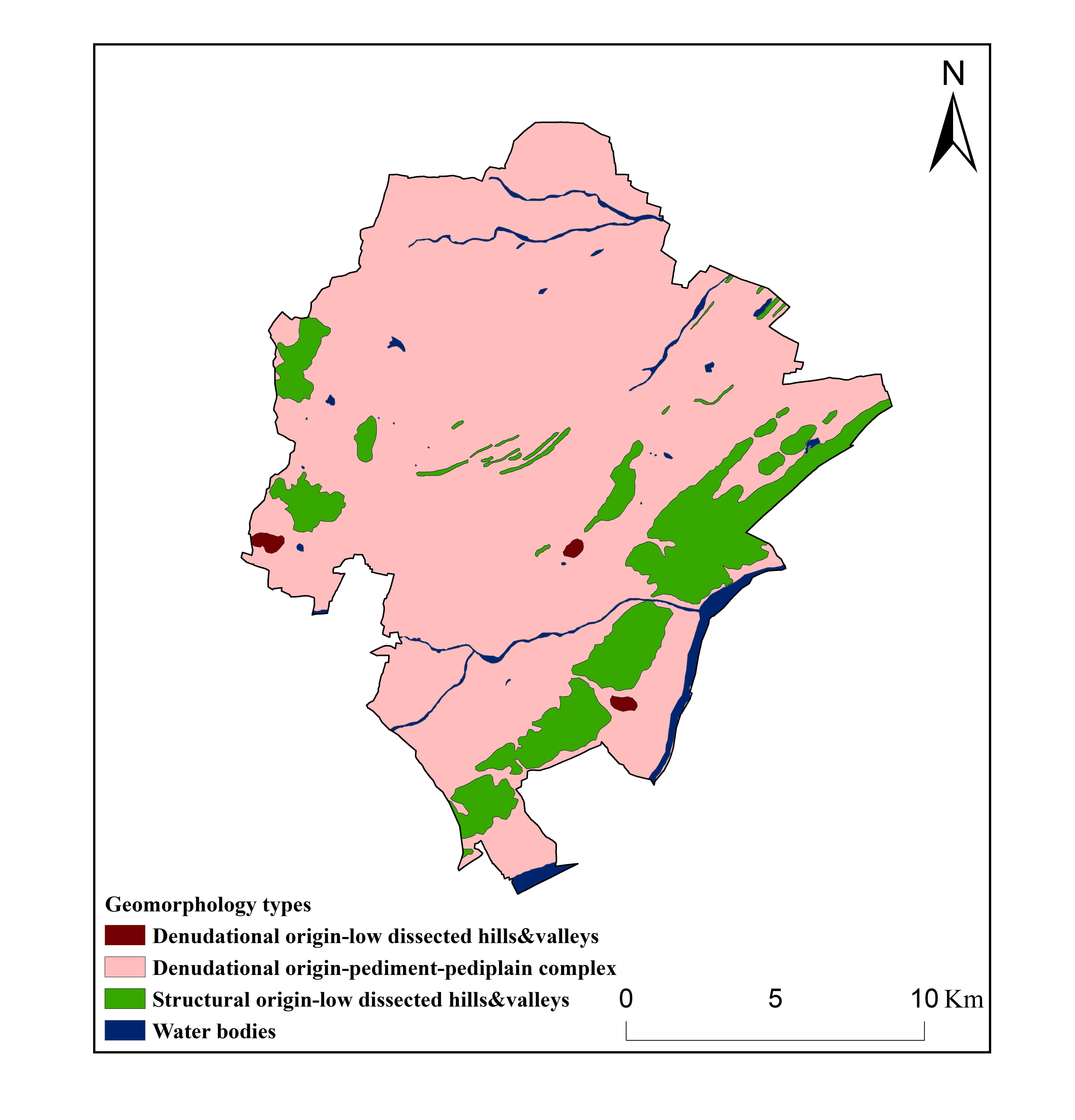
4.2 Geomorphology

Geomorphological maps depict essential landforms and fundamental geology and help comprehension of the procedures, structures and topographical controls identifying with groundwater storage, just as to groundwater possibilities. Such maps portray GWPZs investigation. Satellite imageries have been utilized widely in geomorphologic mapping since the accessibility of early Landsat data, and have for the most part centered around landform grouping, process portrayal and the relationship among landform and procedures, however RS is likewise ready to give data on the area and dispersion of land-shapes, surface-subsurface composition, and topographical elevation (Siva et al., 2017). The present study secured by with a denudational origin with low dissected hills and valleys along with pediment-pediplain complex having with structural origin with low dissected hills (Figure 4).

Figure 4. Geomorphology

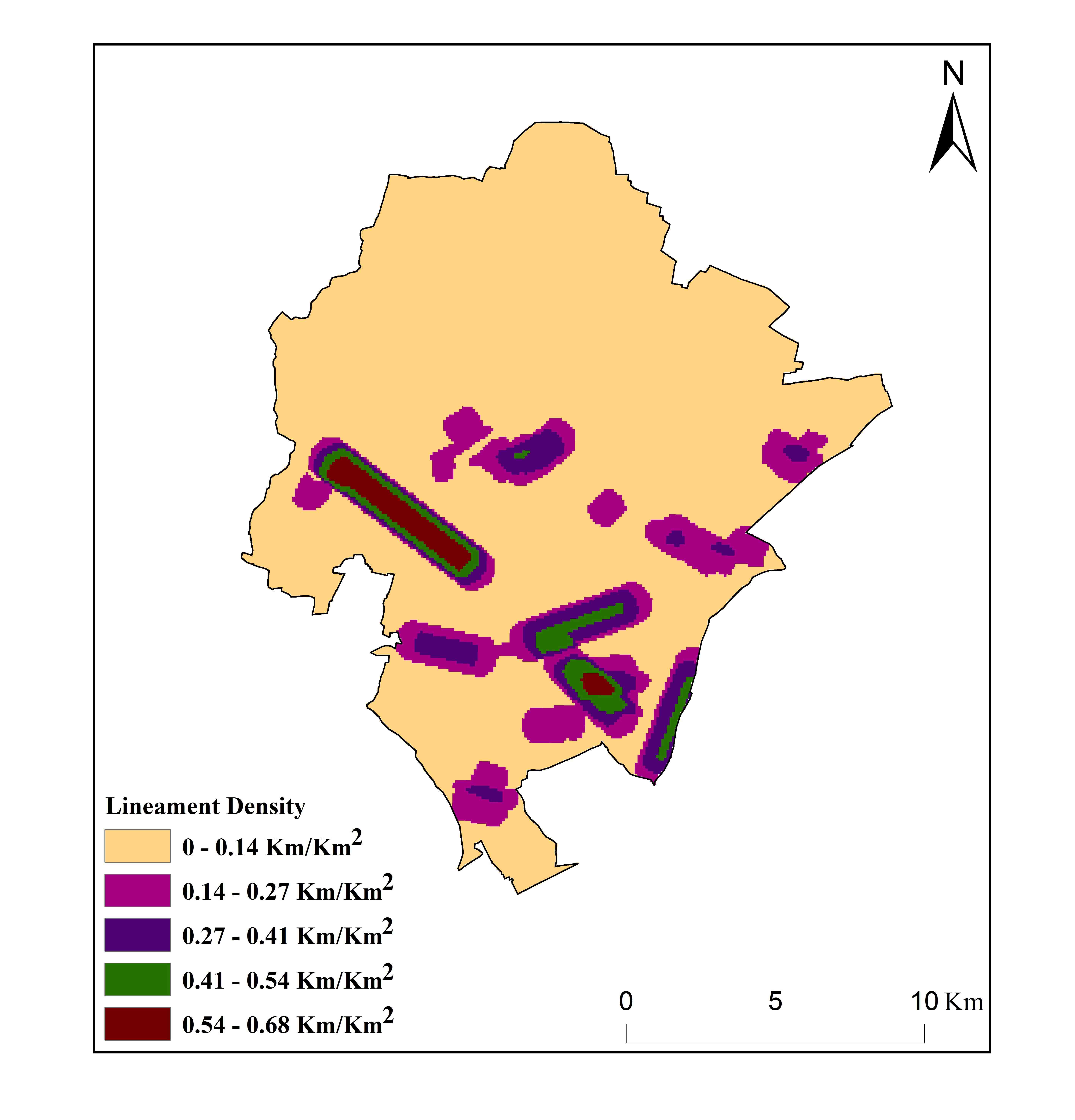
4.3 Lineament Density (LD)

Nearness of lineaments may go about as a channel for groundwater development which consequences in expanded auxiliary porosity and in this way, can fill in as groundwater potential zone. Lineament Density (LD) map is a proportion of the computable length of direct component presented in gird (Shekhar and Pandey, 2015). LD of a region in an indirectly way uncovers the groundwater capability of that territory since the nearness of lineaments, as a rule, signifies a pervious zone. Regions with higher LD are useful for groundwater conservation. In the greater part of the study region, LD changes from 0.14 to 0.68 km/km² which is limited to the area (Figure 5).

Figure 5. Lineament density

4.4 Drainage Density (DD)

Drainage density is a measure of the degree of drainage development within a basin. It reflects the closeness of spacing of channels, attributing due to differential weathering of various formations, relief and rainfall. According to Horton (1932), the DD is defined as the length of stream per unit of a drainage area divided by the area of the drainage basins (Chowdhury et al.,  2008). Low DD is observed in areas of highly permeable sub-soil materials and more DD is observed in areas of weak or impermeable sub-soil materials, scant vegetation and mountain relief. DD is computed according to Horton’s formula is about 1.40 km/km² (Figure 6). Low DD is reflecting permeable sub-surface stratum with dense vegetation and coarse DD show low relief with distinctive landforms.

Figure 6. Drainage density

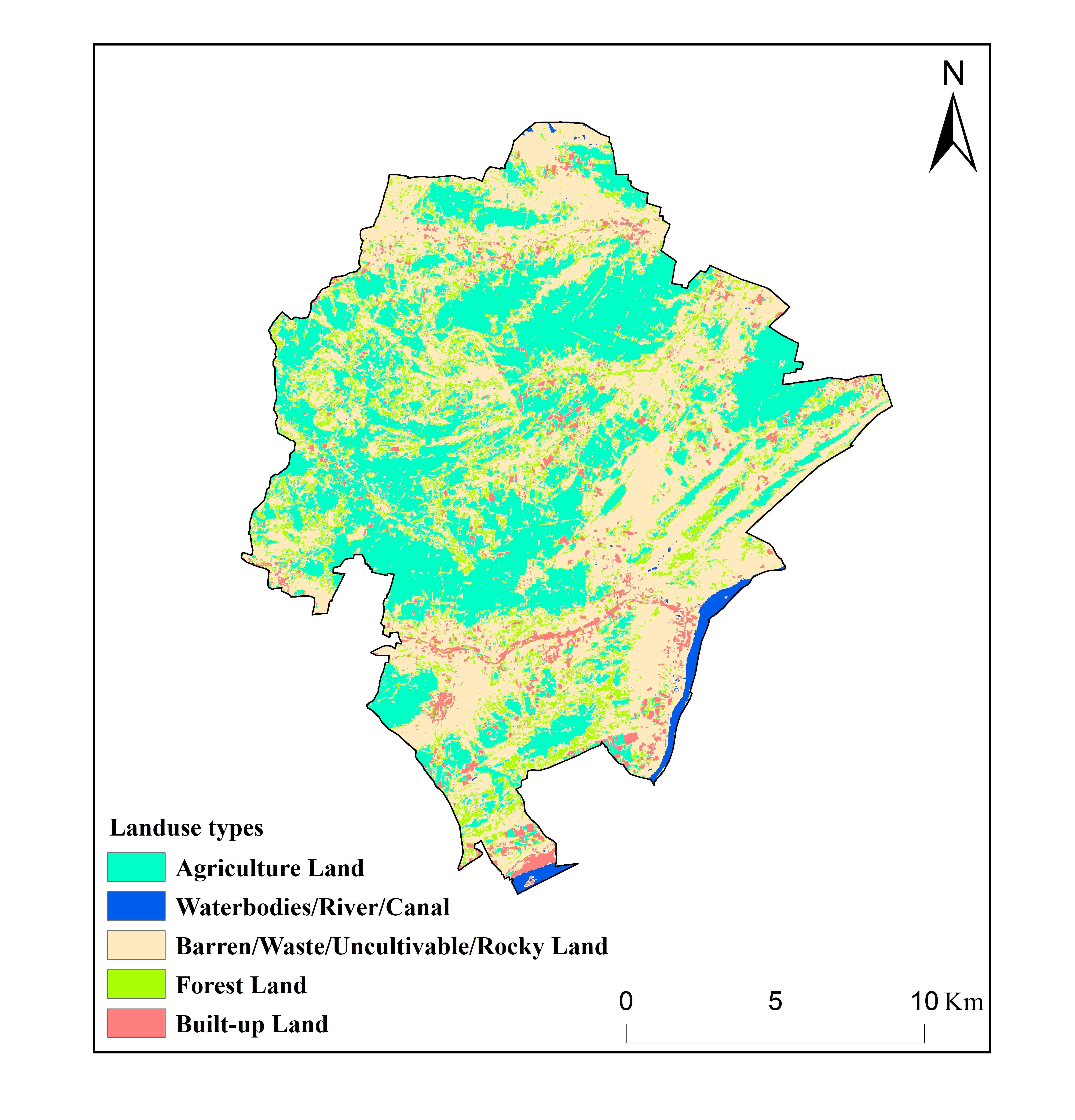
4.5 Land use / Land cover (LULC)

LULC is carried out using ERDAS Imagine 2014 software with supervised classification tool with parallelepiped algorithm method (Figure 7). The probabilities are the correspondent for all classes and the typical conveyance of input bands. However, this method requires a long computation, based on the normal distribution of data in each input bar and tends to exceed the signatures (Basha et al., 2018; Marhaento et al., 2018; Singh et al., 2018; Rajasekhar et al., 2018). According to the signatures, five LULC types have been identified in the study region (Figure 7): (i) Forest, (ii) Agricultural land, (iii) Wastelands, (iv) Built-up lands and (v) Water bodies.

Figure 7. Land use land cover

4.6 Slope

The slope is a measure of changes in surface values ​​at a distance and can be expressed in degrees or as a percentage. DEM raster is a grid in which each cell represents a value compared to a conjoint reference point. After calculating the slope, the maximum difference and slope can be identified. Maps results are used to create a map of biased neighborhood’s usage of ArcGIS 10.4 Spatial Analyst tools (Satheesh kumar et al., 2016). Maximum topographic height (548m) exists in the western and north-western part, causing the highest outflow and therefore much less possibilities of infiltration. The map is categorized into four classes: namely 0-5º (Gentle), 5-15º (Moderate), 15-35º (Steep), >35º (Very Steep) (Figure 8). Large part of the area is gentle and slightly sloping which suggests nearly flat topography of the region. The slope is an essential parameter controls runoff and infiltration of any landscape. Runoff in sloping areas causes less infiltration.

Figure 8. Slopes

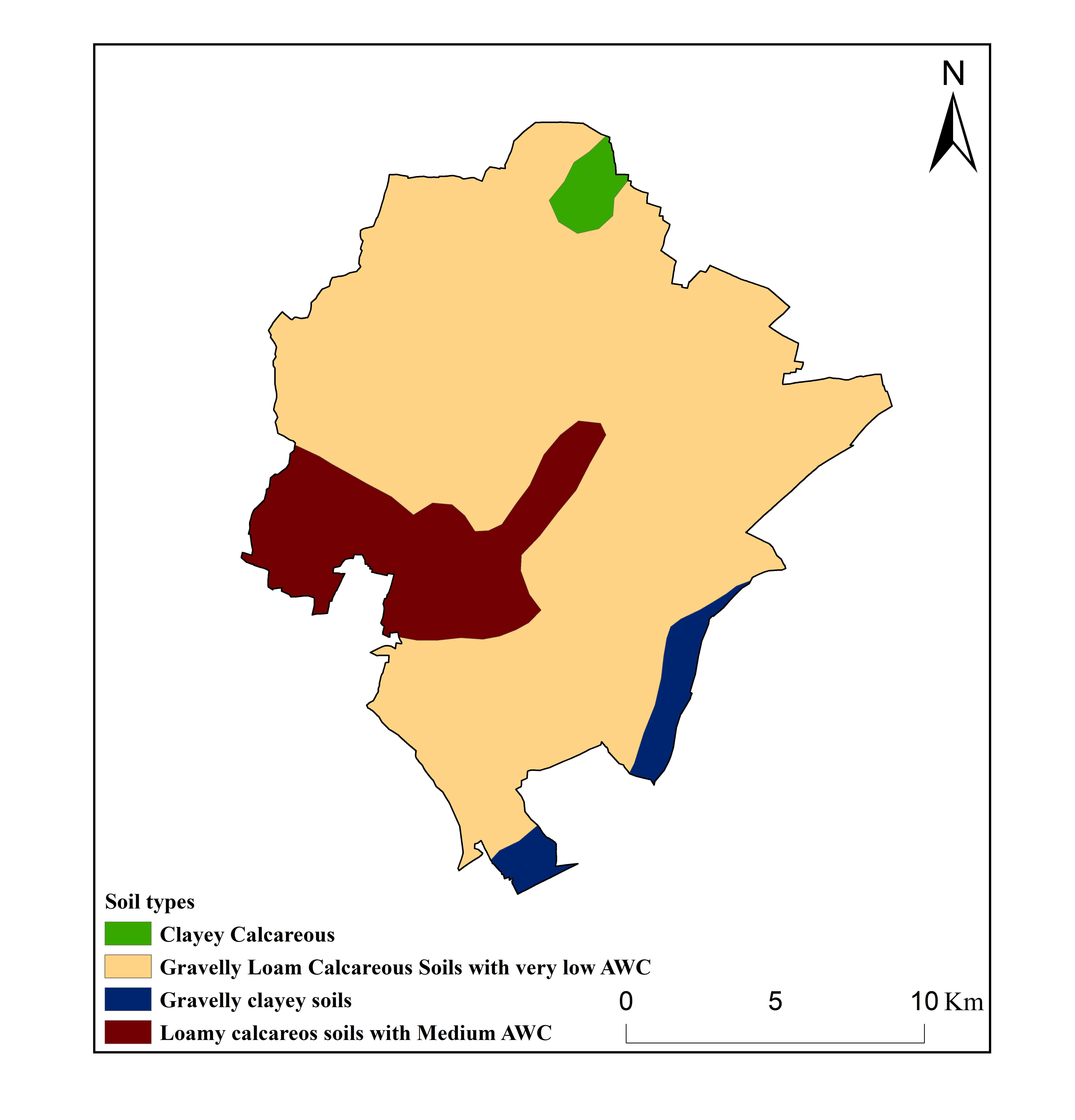
4.7 Soil

Soil map was prepared with the aid of the district groundwater administration (Figure 9). The present study reveals four foremost soil types, viz. gravelly loamy calcareous, loamy calcareous, and minor parts formed by the clay calcareous soils. The major part of the study area covered by the gravelly loamy soils. Ranks for soils have been consigned on the source of their infiltration rate. Loamy calcareous soil has high invasion rate, consequently given higher significance, while the clayey soil has least infiltration rate thus allotted low significance (Nagaraju et al., 2018; Raju et al., 2018; Srinivas et al.,  2015).

Figure 9. Soils

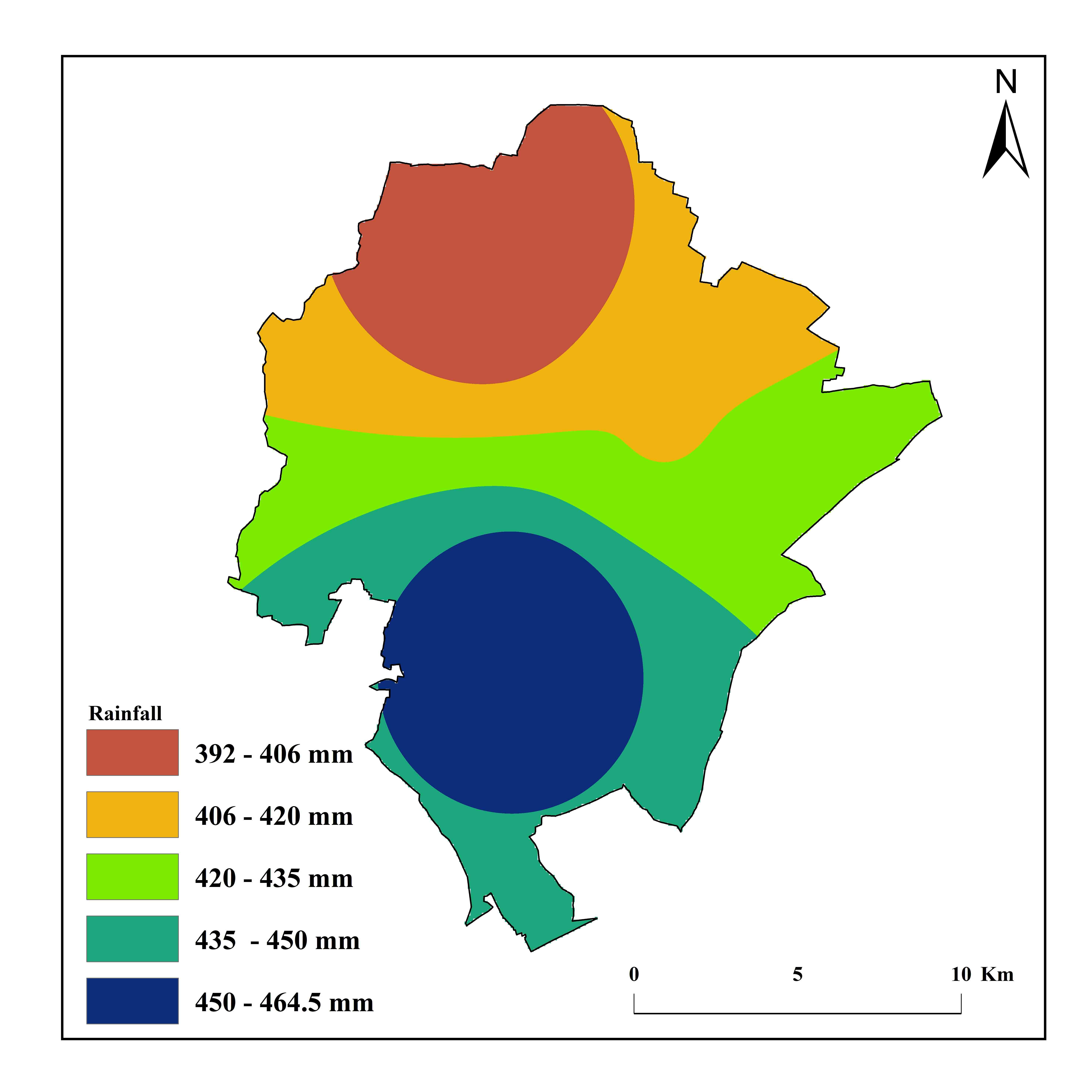
4.8 Rainfall

The yearly average rainfall of the region is about 464.50mm (2017-18). The rainfall map of the present study is shown in Figure 10. The study area depends basically on Northeast monsoon for rainfall (Mundalik et al., 2018; Raju et al., 2018; Rahmati et al., 2015). The Northeast part of the region receives precipitation of around 395mm/year; the Eastern part receives about 400-420mm/year. In the southern part, the recorded precipitation is around 464.50mm/year, and Northeastern part shows low precipitation. The precipitation dispersion alongside the slope gradient in the upstream Southwestern part specifically influences the infiltration rate and henceforth expands the likelihood of GWPZs in the downstream northern part.

Figure 10. Rainfall

4.9 Weightage Analysis and Normalization

Associate the standing of two-layer maps to point out that one in all them has a lot of impact to the groundwater pervasiveness. The pairwise comparison matrix was computed using AHP method (Table 2). The Consistency ratio (CR) was observed to be 0.97 and subsequently thought acceptable. Geomorphology, LULC, DD, soils, geology, LD, slope, and rainfall were generated and assigned appropriate weights as shown in Table 4. To figure out the added substance weights of each criterion and sub-criteria, the similar weight of every criterion and their relating classifications were considered (Table 4). At last, the preservative weight was used to prepare the raster map and GWPZ map was prepared using ArcGIS 10.4 software (Sitender and Rajeshwari, 2011).

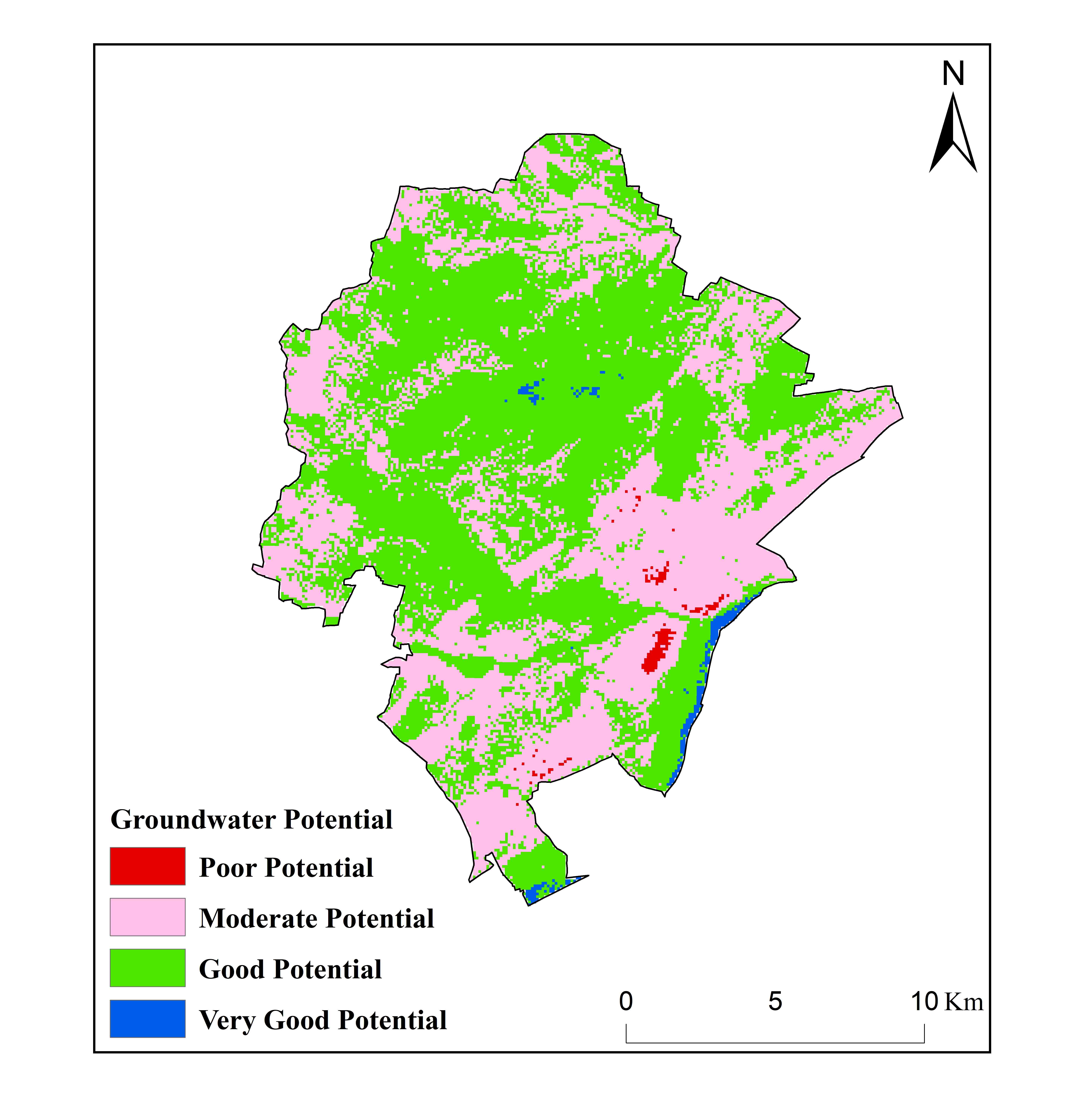
5.10 Groundwater Potential Zones

On the reason of the normalized weights of the distinct features in the thematic maps, the GWPZs were evaluated (Table 3). GWP was ordered into four categories: poor, moderate, good, and very good (Figure 11). The loamy calcareous soils from Northwest parts were show moderate to good GWP. The analysis reveals that only 2.30km² (0.78%) of the study area shows very good GWP, 162.10km² (55.20%) shows good GWP, though 127.78km2 (43.51%) and 1.45 (0.49%) area show moderate and poor GWP, respectively. The good potentials contained weathered granite and hornblende-biotite gneiss, and DD ranges from 0.84-1.12 to 1.12-1.40km/km2. The weathered surface situated within the southern and central part of the present study area has moderate GWP because of the gentle slopes and medium porosity of loamy calcareous soils (Table 5). A wary perception of the GWPZ map demonstrates that the arrangement of groundwater is more or less  replications of the precipitation and geological formations beside slope (Kumar et al., 2015; Mallick et al., 2014; Shankar and Mohan, 2005).

Figure 11. Groundwater potential zones

5 . CONCLUSIONS

The comprehensive performance of AHP technique with GIS is useful for development of an efficient and effective methodology for spatial data management. The integration and analyses of various thematic databases proved useful in the delineation of GWPZ. This study outlines the GWPZ presences by dissecting distinctive thematic maps as impacting factors. The analysis divulges that only 2.30km² (0.78%) of the study area has very good GWP, 162.10km² (55.20%) has good GWP, though 127.78km² (43.51%) and 1.45km² (0.49%) region under moderate and poor GWPs, respectively. The good GWP is considered by the lithology kind such weathered rock formation very and the lower slope within the downstream of the study area. GWPZ map was verified with the well yield data to work out its legitimacy and found that the outcomes are in concurrence with the wells yield data. The pervasiveness of groundwater inside the present study is constrained by DD, geomorphology, geology, slope, and LULC from GIS and straight perception within the field. This GWP map will serve as the basis of information to local authorities and planners about the suitable area for prospective exploration of groundwater and to protect the area from contamination of domestic and industrial activities.

Tables

Figures

Conflict of Interest

Acknowledgements

Abbreviations

References