Keywords

EVI , Ganga , LST , MODIS , NDVI , Python , Vegetation

1 . INTRODUCTION

Uninturrpted monitoring of land surface temperature (LST) and vegetation cover is one of the results of advancement in space technology and it plays an important role for the study of changes with reference to land use and land cover, also a key feature for the study of natural hazards i.e. floods and droughts  (Dall’Olmo and Karnieli, 2002; Julien and Sobrino, 2009; Julien et al. 2011). Climatic factors are the most persuasive among all existing factors, which are found to effect the changes in time and space. By analyzing the land surface temperature and vegetation indices for any region the health of that particular region can be known (Tan et al., 2012). Hence, with the seasonal changes of vegetation indices and temperature provide an pragmatic overview of any region for further study in any aspect. By utilizing the current advance in space technology it is very convenient to get the information about the health of the vegetation, distribution of temperature and rainfall, characteristics of land, changes in gemorphologic features and land use land cover, etc. The products of the Moderate-Resolution Imaging Spectroradiometer (MODIS) is one of the key data sets which already analysed with optimum accuracy (Friedl et al., 2002; Khan et al., 2014; Ovakoglou et al., 2016; Remer et al., 2005; Wang et al., 2007; Wen et al., 2015; Yu et al. 2014; Zhang et al., 2003). We have used automatic and robust techniques for analysis of bulky data for fast and precise outputs. There are many programming languages as well as statistical tools are available i.e. JavaScript, Python, SAS, SPSS Ruby, etc. available for the analysis. Further, Python is one of the best scripting language due to its easy Graphical User Interface (GUI) and English language with user friendly environment to learn and perform effectively (McKinney and Team, 2015; Oguz, 2016). Therefore, GIS and Python is used for understanding surface temperature variations and vegetation changes in the Son-Ganga confluence zone in Middle Ganga Plain (MGP) of Bihar and Utter Pradesh (India).

2 . MATERIALS

2.1 MODIS Satellite Data

The Moderate-Resolution Imaging Spectroradiometer (MODIS) provides data in thirty six (36) spectral bands, wavelength from 0.4µm to 14.4µm with spatial resolutions of 2 bands at 250m, 5 bands at 500m and 29 bands at 1km. It covers the entire Earth within 24 to 48 hours, depending upon the target. MODIS data provides large-scale mapping at global as well as at regional scales.

MOD13Q1 v005 with 12 bands HDF dataset gives first and second band for NDVI and EVI with 250m resolution. MOD11A2 v005 is also in 12 bands of HDF dataset. First and fifth bands of the datasets are having the land surface temperature at 1000m resolution for daytime and nighttime, respectively.

2.1.1 Vegetation Indices (16 ­Days Level 3 Global 250m): MOD13Q1

MOD13Q1 datasets are intended to provide constant spatial and temporal evaluations of vegetation covers. Blue, red, and near-infrared bands, capturing information at 0.469µm, 0.645µm and 0.858µm, respectively and provides daily vegetation indices at global scale (Table 1). The study area is a part of floodplain of Son-Ganga confluence, where vegetation behaviour is dynamic in nature. Therefore, the minimum interval of satellite data with good resolution (250m) has been taken into consideration.

The dataset, MOD13Q1, provides Normalized Difference Vegetation Index (NDVI) (Equation (1)) and Enhanced Vegetation Index (EVI) (Equation (2)) products for continuous monitoring of vegetation conditions. NDVI defines the density of greenness for a patch of any region/land. The pigment called chlorophyll available in every plant leaves, absorbs visible light, 0.4 to 0.7µm, for process to photosynthesis. But the structure of the leaves reflects NIR light, 0.7 to 1.1µm. Dense vegetations affect these wavelengths, visible and NIR, of light, through these affects the NDVI for any region has been monitored successfully. While, advance methods utilized in EVI provides minimum variations of canopy background and maintains the sensitivity for dense vegetation environment. It also minimizes the contamination in residual atmosphere, available due to smoke and patches of thin clouds.

\(NDVI=(NIR-Red) / (NIR+Red)\)         (1)

where, NDVI  stands for Normalized Difference Vegetation Index, NIR  is Near Infrared and Red is red band of the spectrometer.

\(EVI= G\times {(NIR - Red) \over (NIR+C1 \times Red-C2 \times Blue + L)}\)            (2)

where, NIR, red or blue are reflectances with atmospheric correction, L is the canopy background and C1, C2 are the aerosol resistance coefficients, which uses the blue band for correction in the red band for aerosol influences. The aerosol resistance coefficients, adopted in the algorithm are- C1 = 6, C2 = 7.5, L=1, and G (refere as gain factor) = 2.5.

2.1.2 Land Surface Temperature (08 ­Days Global 1km): MOD11A2

Land Surface Temperature (LST) is a measurement of skin temperature of any land surface, which is recorded by the sensors mounted in any satellite or a hand handled device. The estimations from any sensor are also depending on the albedo, type and cover of vegetation and moisture in soil. It’s a combination of bare soil and vegetation temperatures. Due to aerosol load modifications, cloud cover, and daytime variation of illumination; the rapid changes found in incoming solar radiation which caused the quick variations in recorded LST also.

The dataset, MOD11A2 provides Land Surface Temperature (LST) and Emissivity at 8-days interval which is composed by the average values of daily 1km LST product- MOD11A1 and it’s available at 1km in Sinusoidal projection. It stores the information of day- and night-time LSTs in Band 31 and 32. Table 2 describes the details of the LST data. Temperature varies due to continuous deposition of sediment in the floodplains and 8-days interval data of MODIS was found helpful for this study.

3 . STUDY AREA

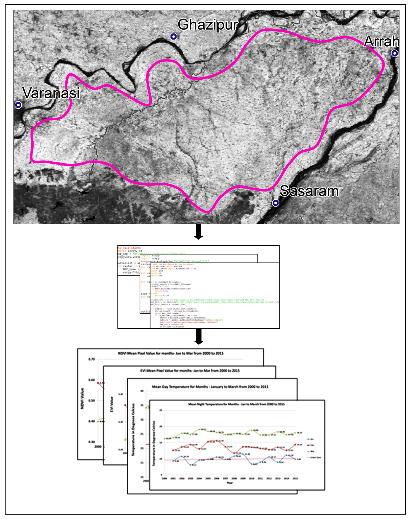
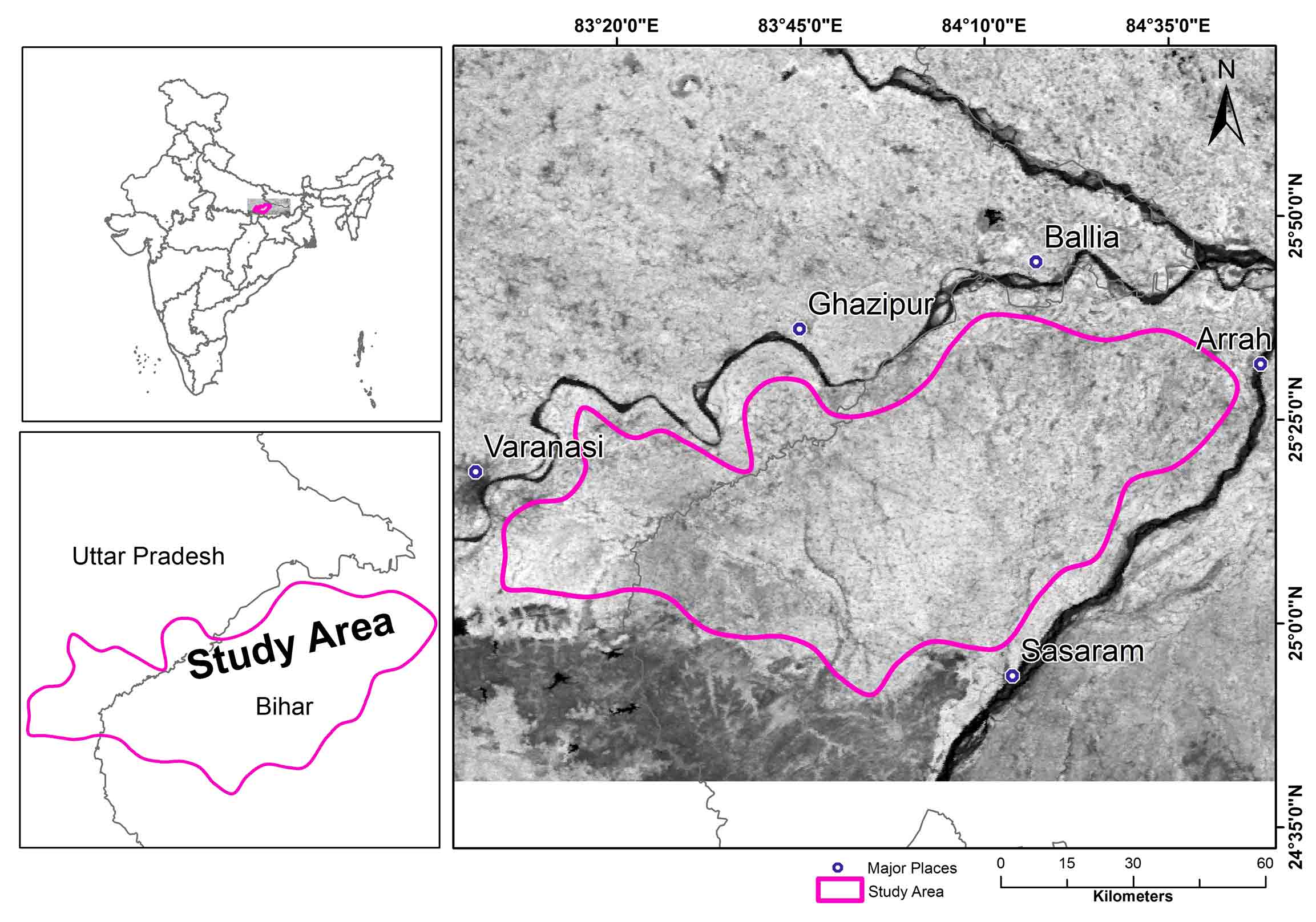
The study area counters from 25°40'18.438"N, 83°3'54.026"E to 24°51'50.725"N , 84°41'41.285"E. It covers an area of ~ 8000 sq. km., which is almost 10.6% of total floodplain of Son-Ganga confluence zone (75,000 km²). The maximum temperature is observed in May and minimum in January. This area received moderate to high rainfall (450-700 mm). The study area has alluvium soil with good agriculture. Major crops are rice, wheat and sugarcane. The major cities are Varanasi, Ghajipur and Ballia from Uttar Pradesh and Patna, Arrah and Sasaram from Bihar (Figure 1).

Figure 1. Study area: Son Ganga River

4 . METHODOLOGY

Total 1098 datasets of MOD13Q1 (368 tiles): NDVI and EVI and MOD11A2 (730 tiles) were used for LST estimation were downloaded from Earth Data Centre, NASA in Hierarchy Data Format (HDF) using WGET freeware (Didan, 2015; Zhang et al., 2014).    

LST product, scale factor of 0.02, was analyzed over the period starting from 05 March, 2000 to 27 December, 2015. NDVI/EVI products of MODIS used in the study for the period during 18 February, 2000 to 19 December, 2015. To rescale the values of temperature are multiplied with 0.02 while the values for NDVI and EVI are multiplied with 0.0001 for better understanding the results. Further the temperature values were converted into Degree Celsius from Kelvin.

Resampling and clipping, in rectangular shape, for study area, of HDF files were performed using MODIS R tool. Also, for better functionality and further uses, the HDF datasets were converted into Tagged Image File Format (TIFF) files and extraction of Day and Night from MOD11A2 datasets and NDVI and EVI from MOD13Q1 datasets in TIFF format were completed using MODIS R tool.

Processing of input data were done in Python and MS-Excel. The modules used for this study, ARCPY, NUMPY, GDAL, MATPLOTLIB, etc., are very crucial and user friendly to use for calculation of large heterogeneous data with single script. The other tools which have been used for this study are WGET and MODIS R.

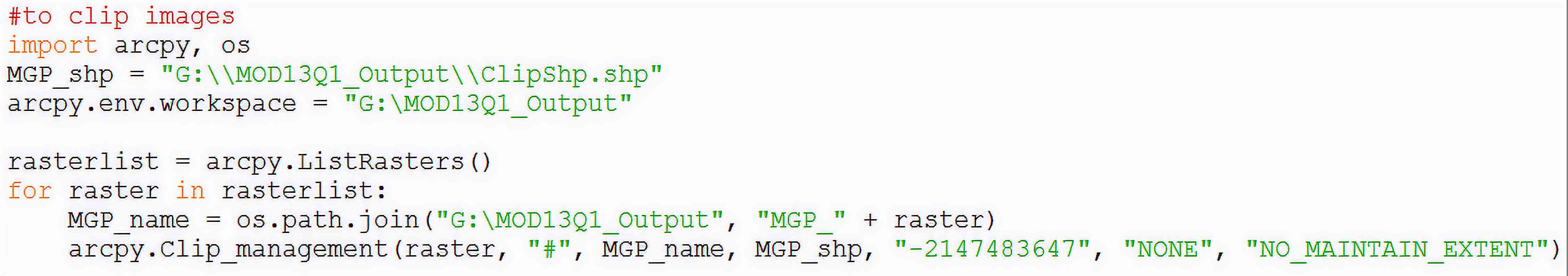
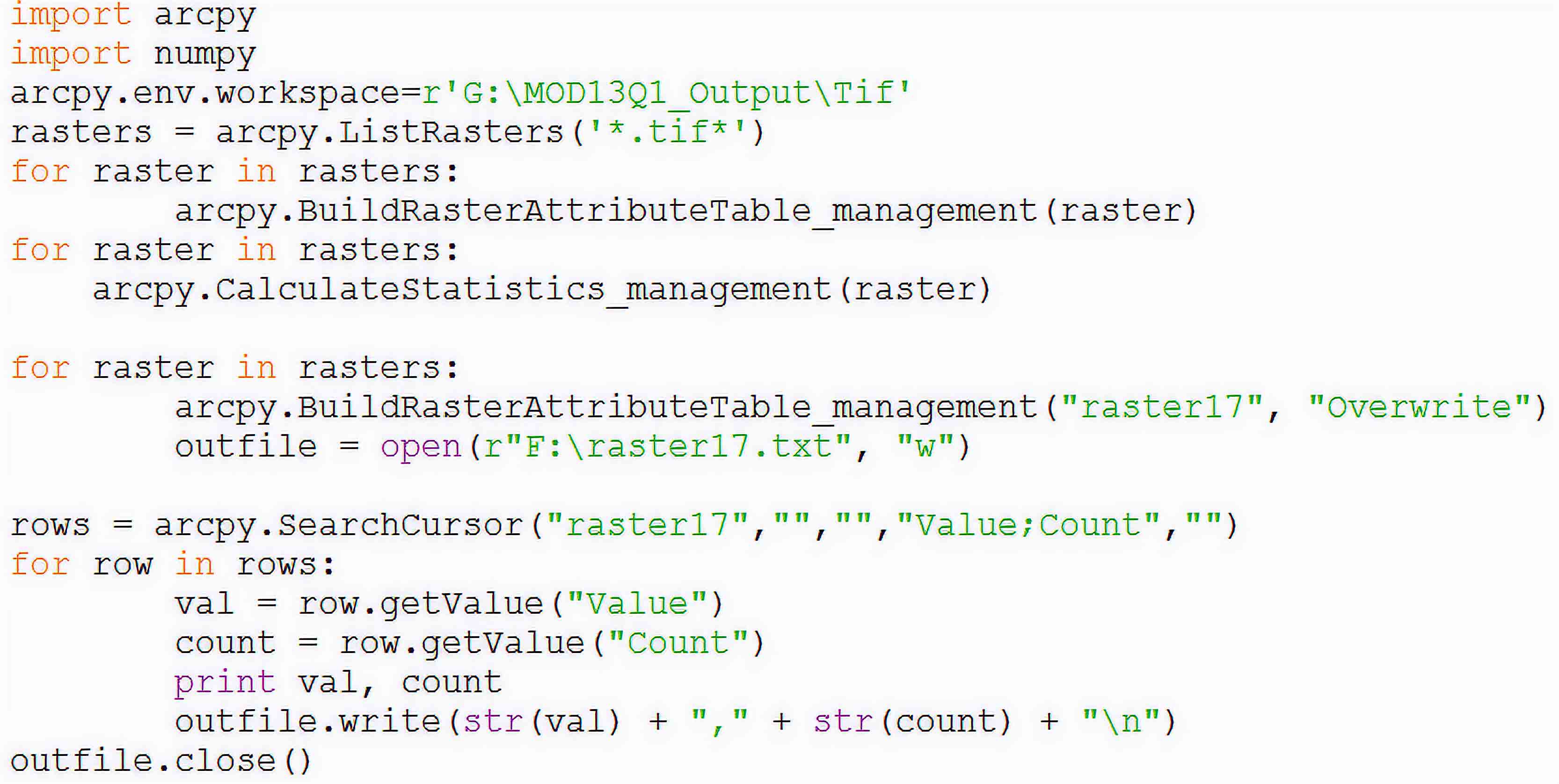
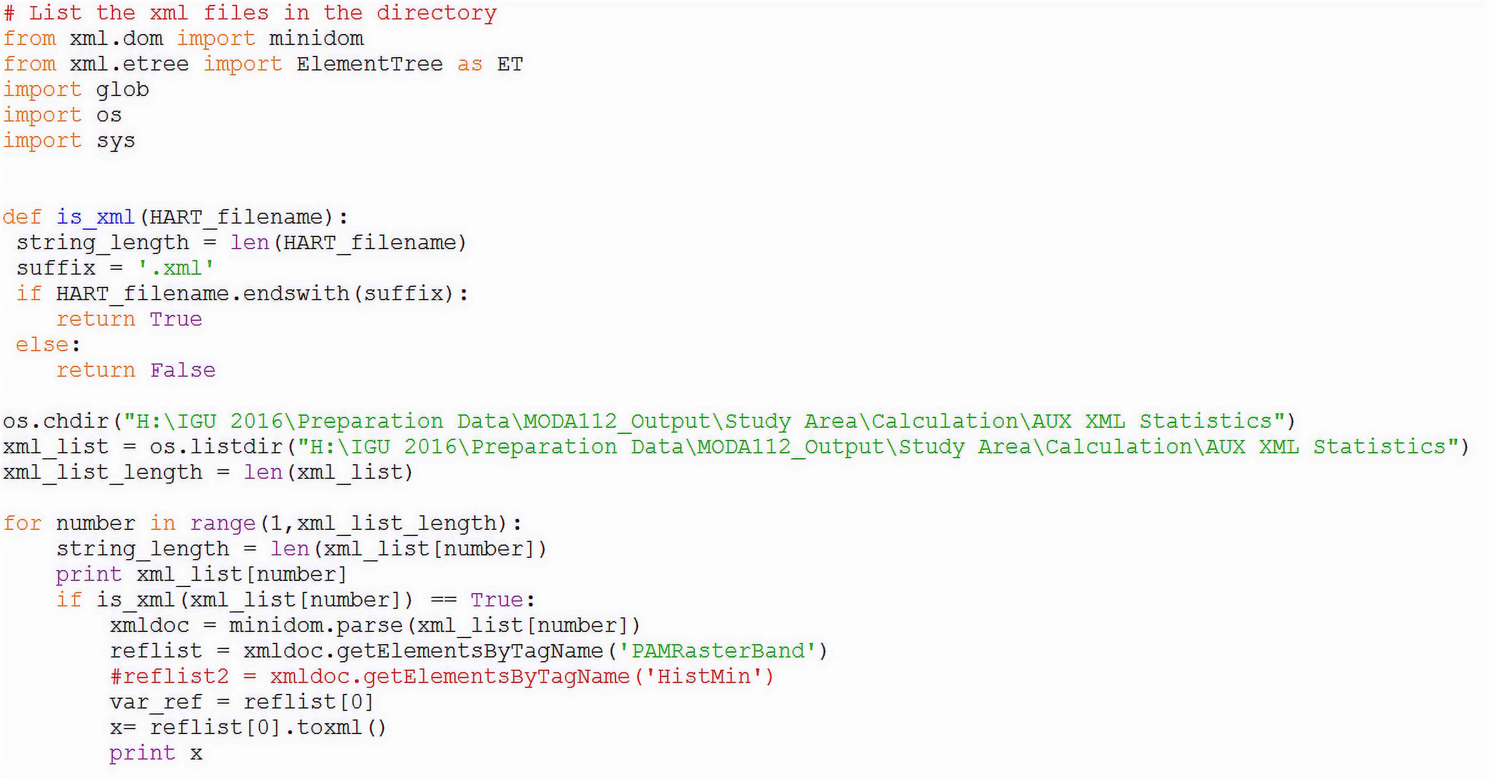
The script details describing the clipping of Raster files using shape file (Figure 2).  The general statistics, mean, maximum and minimum, etc., of individual image was calculated using the Python script (Figure 3). Calculated values were saved into Extended Markup Language (XML) for feasible uses of values further sample data value of calculated statistics of single TIFF file (Figure 4) (Clauss et al., 2016; Huang  et al., 2012).

Figure 2. Script for extracting of raster dataset (in Python)

Figure 3. Script for calculating statistics from extracted images

Figure 4. Script for extraction of XML data from raster files

Cause of overcast weather (cloud cover) during monsoon period (June to September) and some data were not recorded correctly due to some radiometric and geometric errors. These data were removed from the corrected data table for better result.

The resultant data for different period, 16 days for NDVI and EVI and 8 Days for LST Day and Night time, was compiled and averaged on monthly basis from resultant data and was plotted in excel.

5 . RESULTS AND DISCUSSION

Results are described into four sections: 1) Mean Pixel Temperature of Daytime (2000 to 2015), 2) Mean Pixel Temperature of Nighttime (2000 to 2015), 3) Mean Pixel Value NDVI (2000 to 2015), and 4) Mean Pixel Value EVI (2000 to 2015).

5.1 Mean Pixel Temperature of Daytime (2000 to 2015)

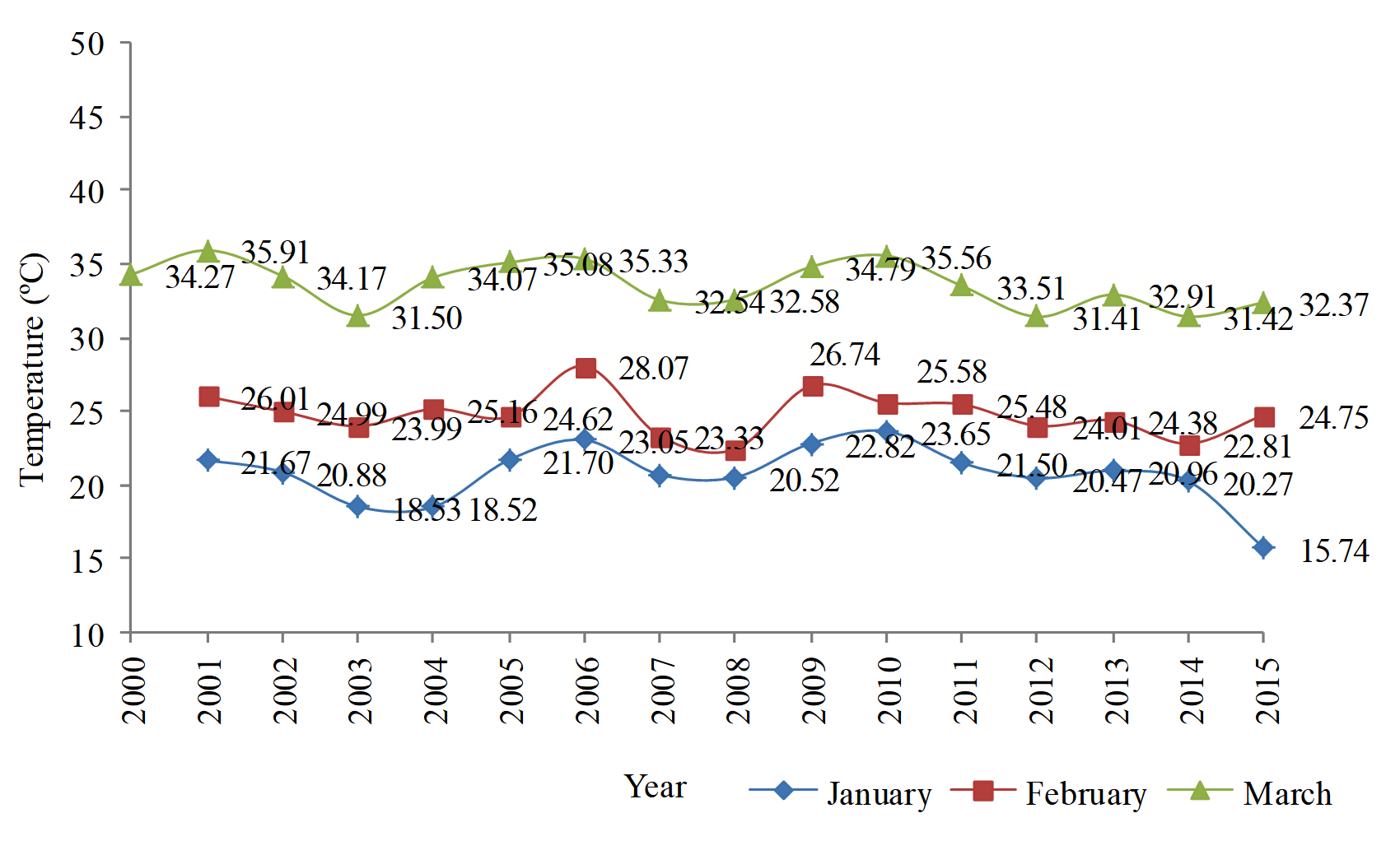
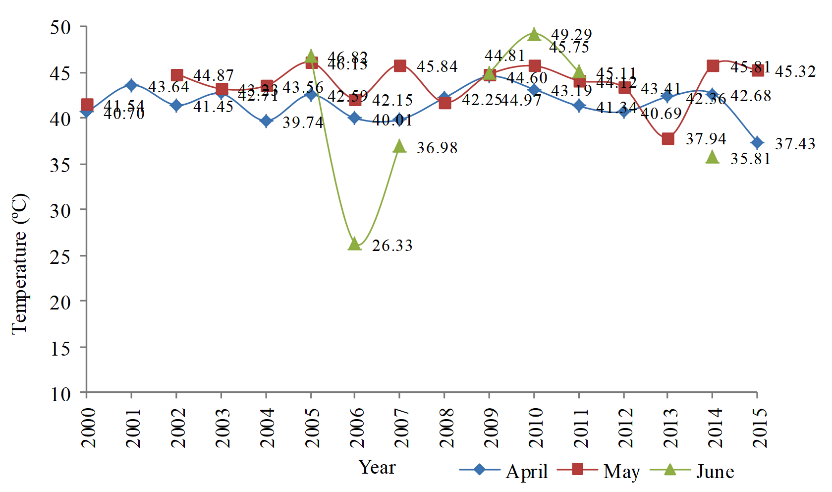
The average day time temperature for the month of January has been fallen for around 2°C (Figure 5). While for the month of February and March the declining trend is almost same. The average day temperature for the month of April was decreased for almost 4°C (Figure 6). Month of May 2015 is recorded high temperature in comparison of 2001. Due to cloud cover on arrival of monsoon in Indian subcontinent the data could not recorded for the month of June and reliability even on the recorded data for the plotted years cannot be trusted.

Figure 5. Mean Daytime Temperature: January to March (2000 to 2015)

Figure 6. Mean Daytime Temperature: April to June (2000 to 2015)

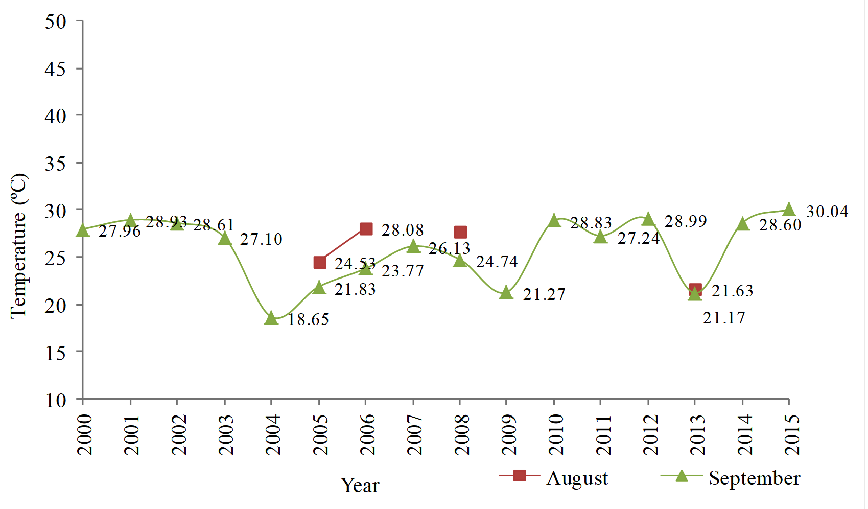
The average day temperature for the month of July and August was not recorded due to cloud cover (Figure 7). September is showing lowest record for the year 2004 and about 30 °C for 2015.

Figure 7. Mean Daytime Temperature: July to September (2000 to 2015)

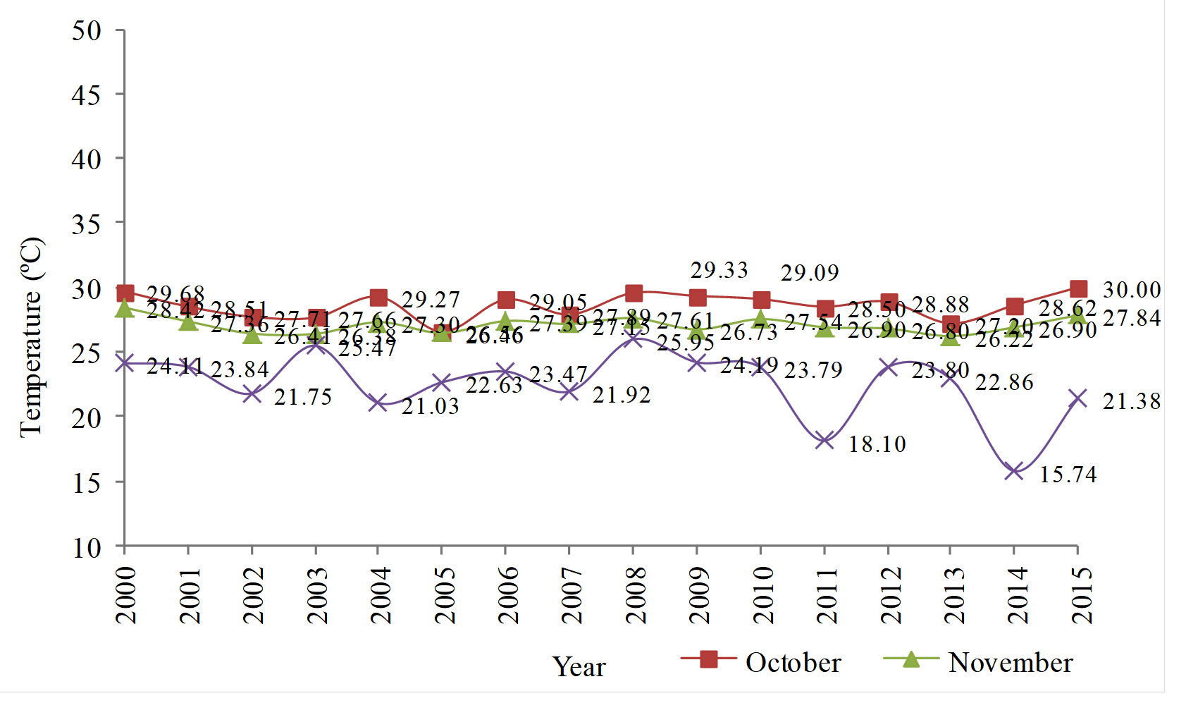
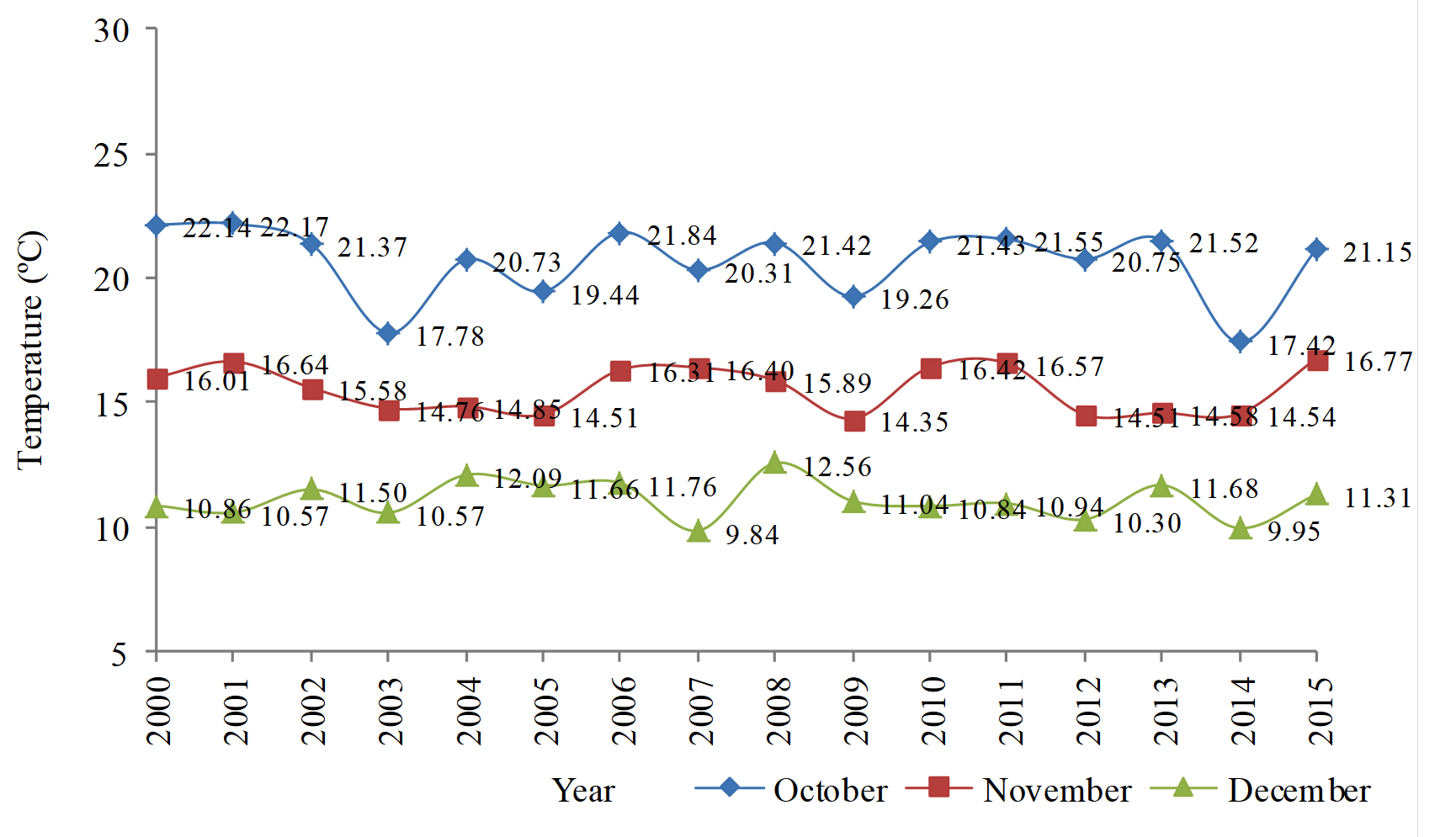
The average day temperature for the months of October and November was not changed much during 2000 to 2015 (Figure 8). December is showing declining trend continuously during the recorded period.

Figure 8. Mean Daytime Temperature: October to December (2000 to 2015)

5.2 Mean Pixel Temperature of Nighttime (2000 to 2015)

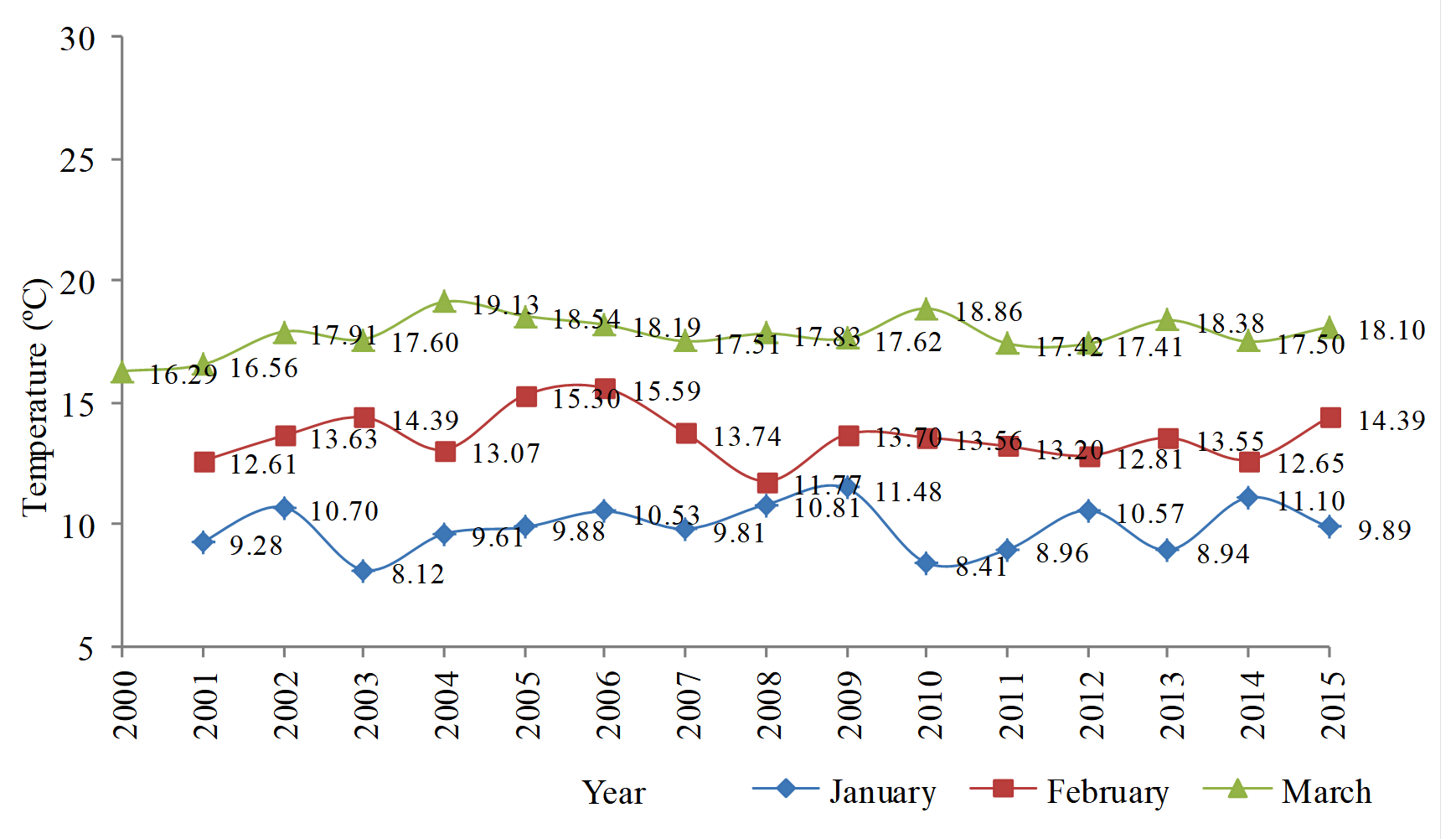
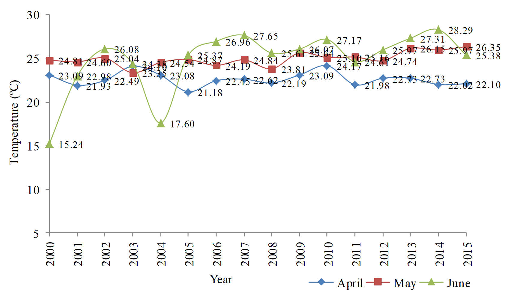
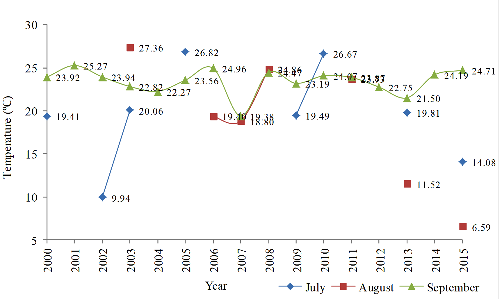
The zigzag values ranging from 9 to 10 for the months of January, 12 to 14 for February and 16 to 18 for the month of March during the study period (Figure 9). There is no major change can be seen for the months of April and May but the value for June in year 2000 is extremely low, 15.24 °C, due to rain or other factor (Figure 10). Also, the year 2004 for June shows low temperature, 17.40 °C, in comparison of general temperature recorded for June. Apart from these two years, 2000 and 2004, the average pixel temperature was found normally during the study period. Again, the July and August data for the study period could not be plotted due to cloud cover (Figure 11). The lowest average pixel temperature, 19.38°C, for the month of September was recorded in the year of 2007. While for the rest of years it was ranging between 21 to 25°C. Daytime temperature is well distribution for the months of October, November and December during year period (Figure 12). Slight decrease in temperature can be seen in the month of October daytime average pixel temperature.

 

Figure 9. Mean Nighttime Temperature: January to March (2000 to 2015)

 

Figure 10. Mean Nighttime Temperature: April to June (2000 to 2015)

 

Figure 11. Mean Nighttime Temperature: July to September (2000 to 2015)

 

Figure 12. Mean Nighttime Temperature: October to December (2000 to 2015)

 

5.3 Mean Pixel NDVI (2000 to 2015)

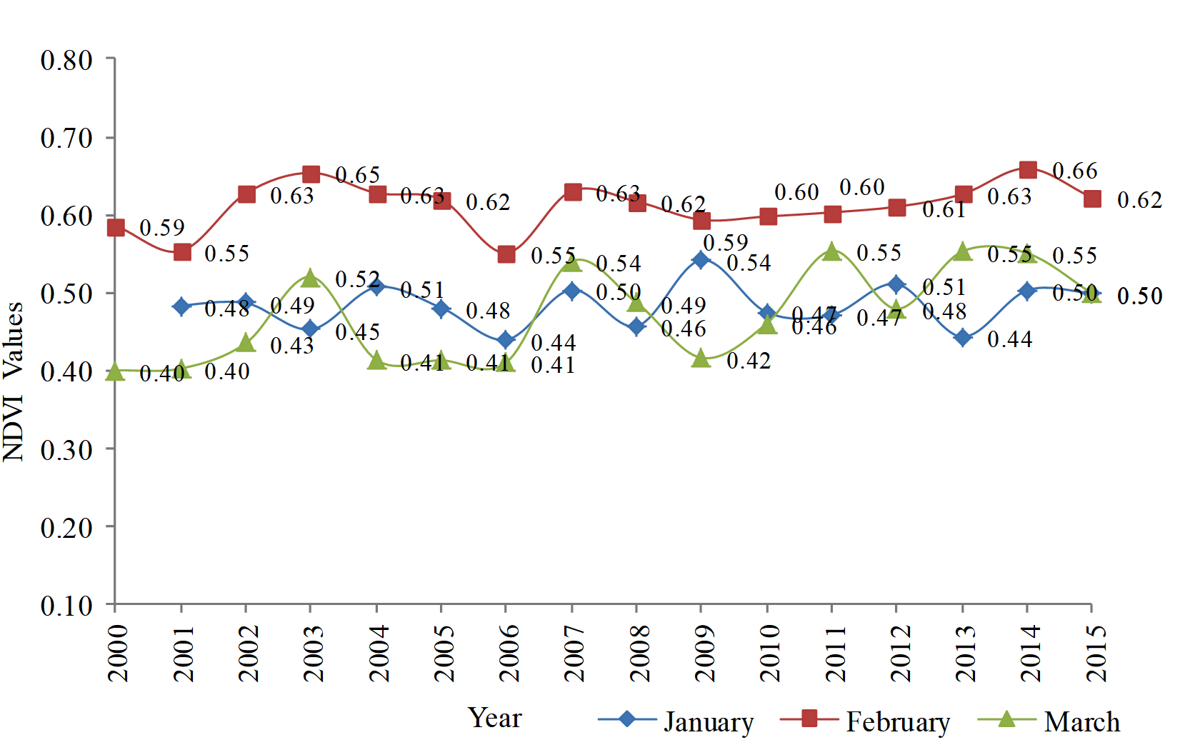
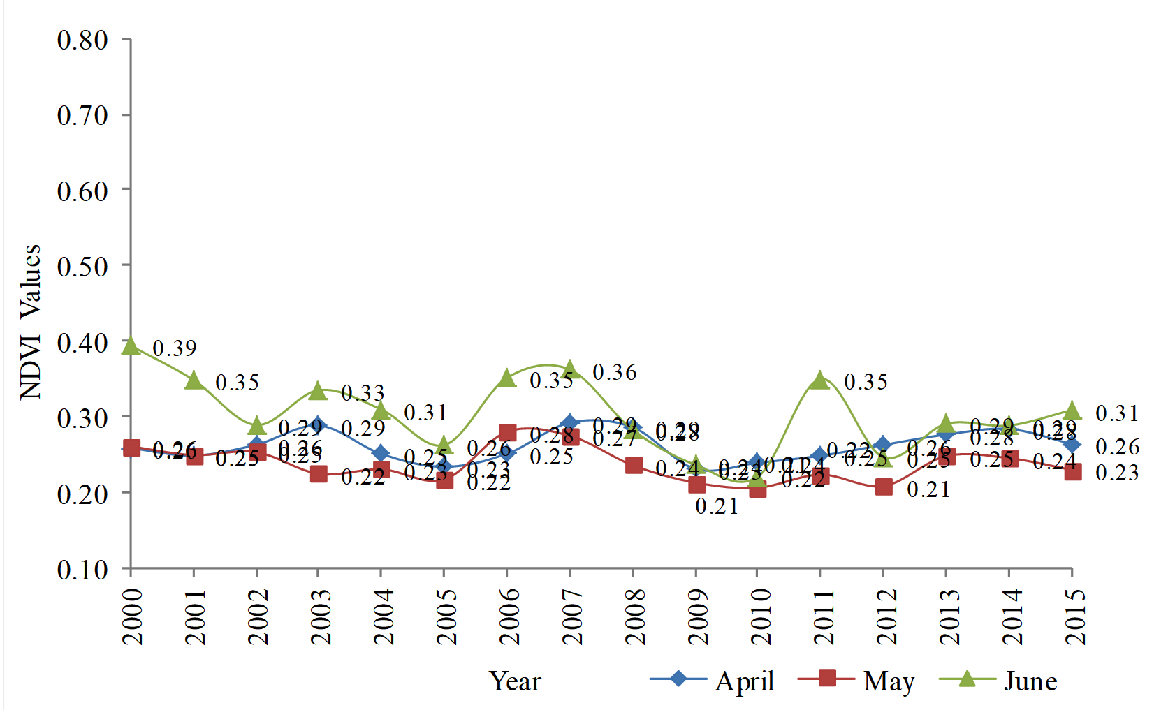
The mean pixel value for NDVI is increased for the months January, February and March from year 2000 to 2015 (Figure 13). The values for all three months are ranging from 0.40 to 0.60, which reflect a good quantity of chlorophyll content in leaves available in the study area. The mean pixel values for NDVI is almost same for the months April and May but in the month of June the recorded data is showing a huge crest and during study period (Figure 14). It starts with 0.39 and goes down up to 0.2 and ends on 0.31.

Figure 13. Mean NDVI Pixel Value: January to March (2000 to 2015)

Figure 14. Mean NDVI Pixel Value: April to June (2000 to 2015)

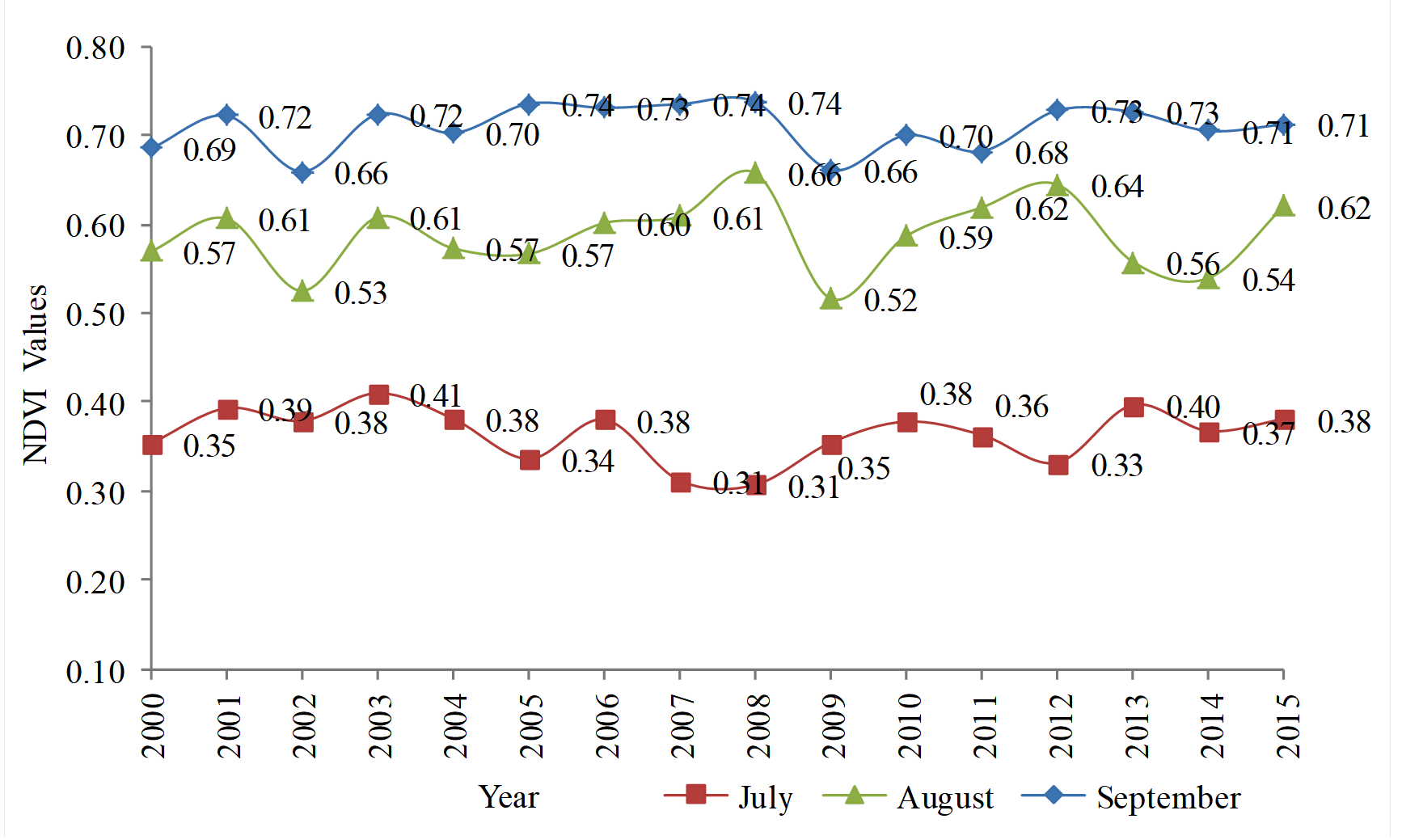
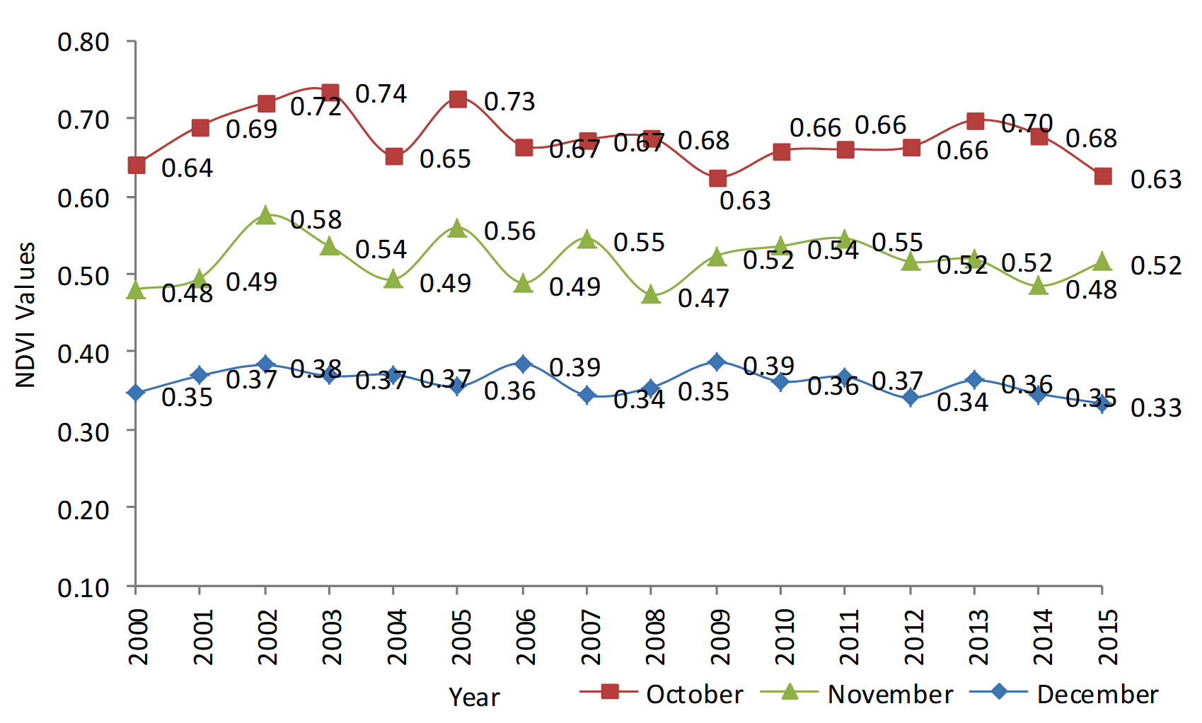
A symmetrical distribution of recorded values can be noted for the months July, August and September during the study period (Figure 15). The mean pixel value for the month of July is ranging from 0.30 to 0.40. For August it is ranging from 0.5 to 0.6 and for the month of September it is stretching from 0.65 to 0.70. The data for the month of September shows a good amount of chlorophyll content is available in the study area. The trend for October, November and December is almost straight during the study period (Figure 16). In October, NDVI values is ranging from 0.60 to 0.70 and for November it is ranging from 0.40 to 0.50 while for the month of December it is stretching from 0.30 to 0.40 due to less duration of sunlight availability.

Figure 15. Mean NDVI Pixel Value: July to September (2000 to 2015)

Figure 16. Mean NDVI Pixel Value: October to December (2000 to 2015)

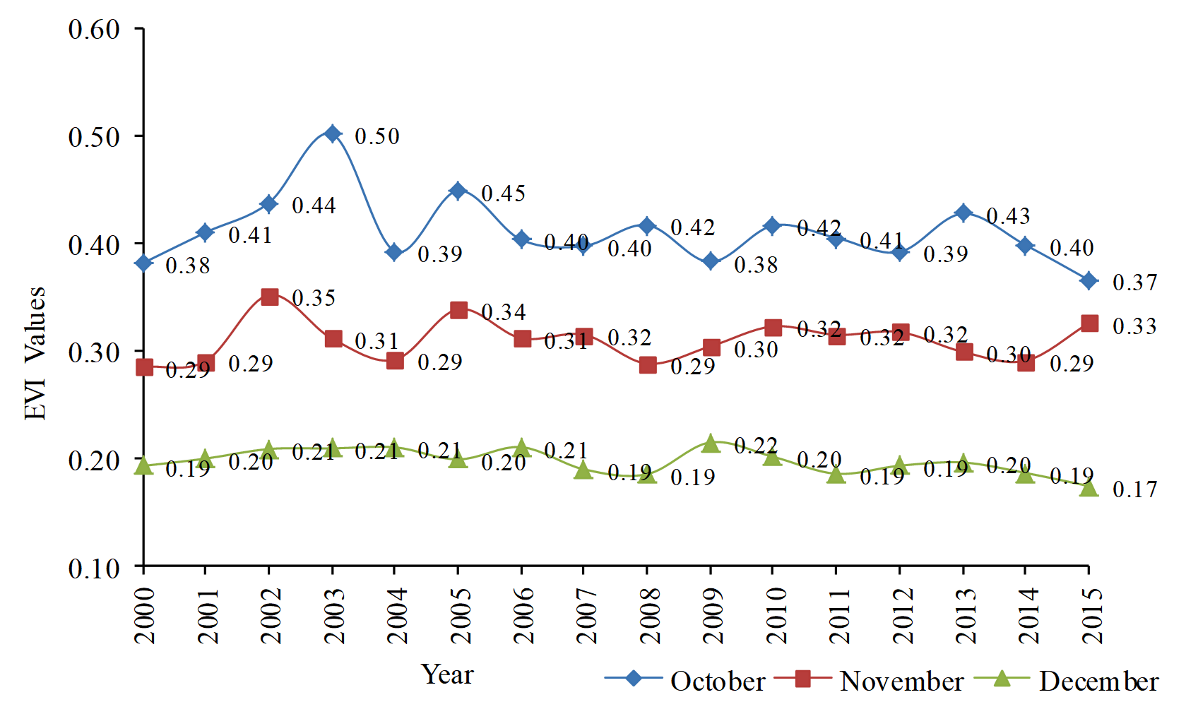
5.4 Mean Pixel EVI (2000 to 2015)

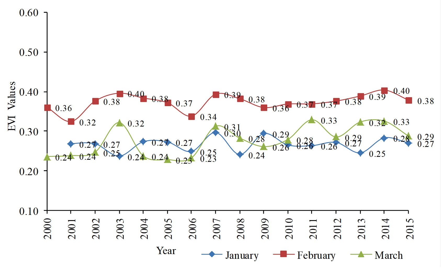
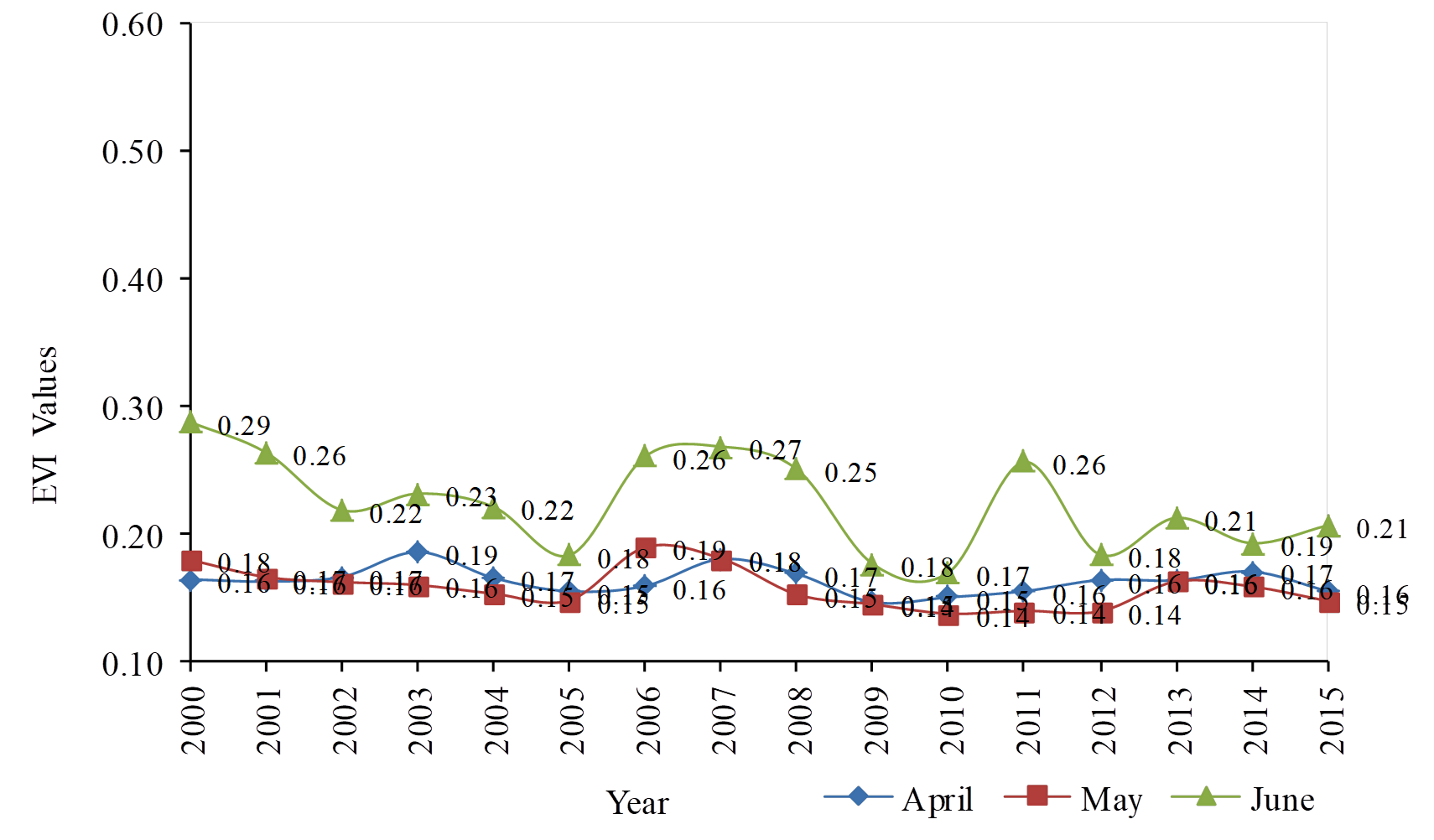
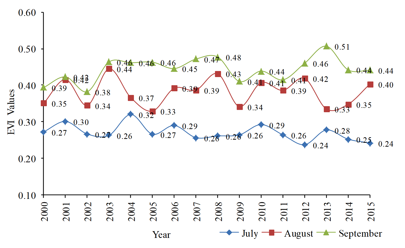
The increasing trend is noticed in EVI values for all three months, January, February and March (Figure 17). For all months the values are ranging from 0.20 to 0.35 during the study period. The declining trend was observed for the months, April to June during the study period (Figure 18). EVI values are ranging from 0.15 to 0.30 for all three months. The trend for month of July is declining while values for the months of August and September are recorded in increasing mode (Figure 19). EVI values are ranging from 0.20 to 0.50 for all three months. The trend for these months is almost straight during the study period as same pattern was recorded in NDVI (Figure 20). In October, NDVI values are ranging from 0.35 to 0.50 and for November it is ranging from 0.30 to 0.40 while for the month of December it is stretching from 0.17 to 0.220 due to less duration of sunlight availability. Daytime LST indicates a slightly decreasing monthly trend with average pixel temperature 28.47°C on March 5, 2000 and 20.49°C on December 27, 2015 and nighttime LST shows the declining monthly trend with average pixel temperature 15.14°C and 9.61°C on the same corresponding dates. NDVI values for the area reveals an increasing trend (NDVI ranges between 0.09-0.23) and EVI during the same period also shows the same rising monthly trend (EVI ranges between 0.26-0.34).

Figure 17. Mean EVI Pixel Value: January to March (2000 to 2015)

Figure 18. Mean EVI Pixel Value: April to June (2000 to 2015)

Figure 19. Mean EVI Pixel Value: July to September (2000 to 2015)

Figure 20. Mean EVI Pixel Value: October to December (2000 to 2015)

6 . CONCLUSION

Analysis over large satellite data is still a big challenge with the availabe Remote Sensing and GIS techniques. A high end programming language like Python can calculate the bulky data efficiently with precision. In this study, about 100 gigabyte (GB) satellite data of MODIS was used and the approach for this study was to establish the correlation between NDVI and LST using Python and other available freeware. The study was completed on low resolution images, 250 m and 1000 m, of MODIS satellites due to large study area (~8000 sq.km).

Average pixel temperature of daytime and nighttime has been decreased throughout the study period. As well as NDVI and EVI show the increasing trend significantly cuase of increasing temperature and precipitation. Increasing values of NDVI/EVI and decreasing trend of LST in the area least affected by human settlements (because of frequent flooding around confluence zone) indicates an inverse relationship between temperature and vegetation. This study signifies the use of satellite derived data in environmental monitoring in floodplain areas.

Tables

Figures

Conflict of Interest

Acknowledgements

Abbreviations

References