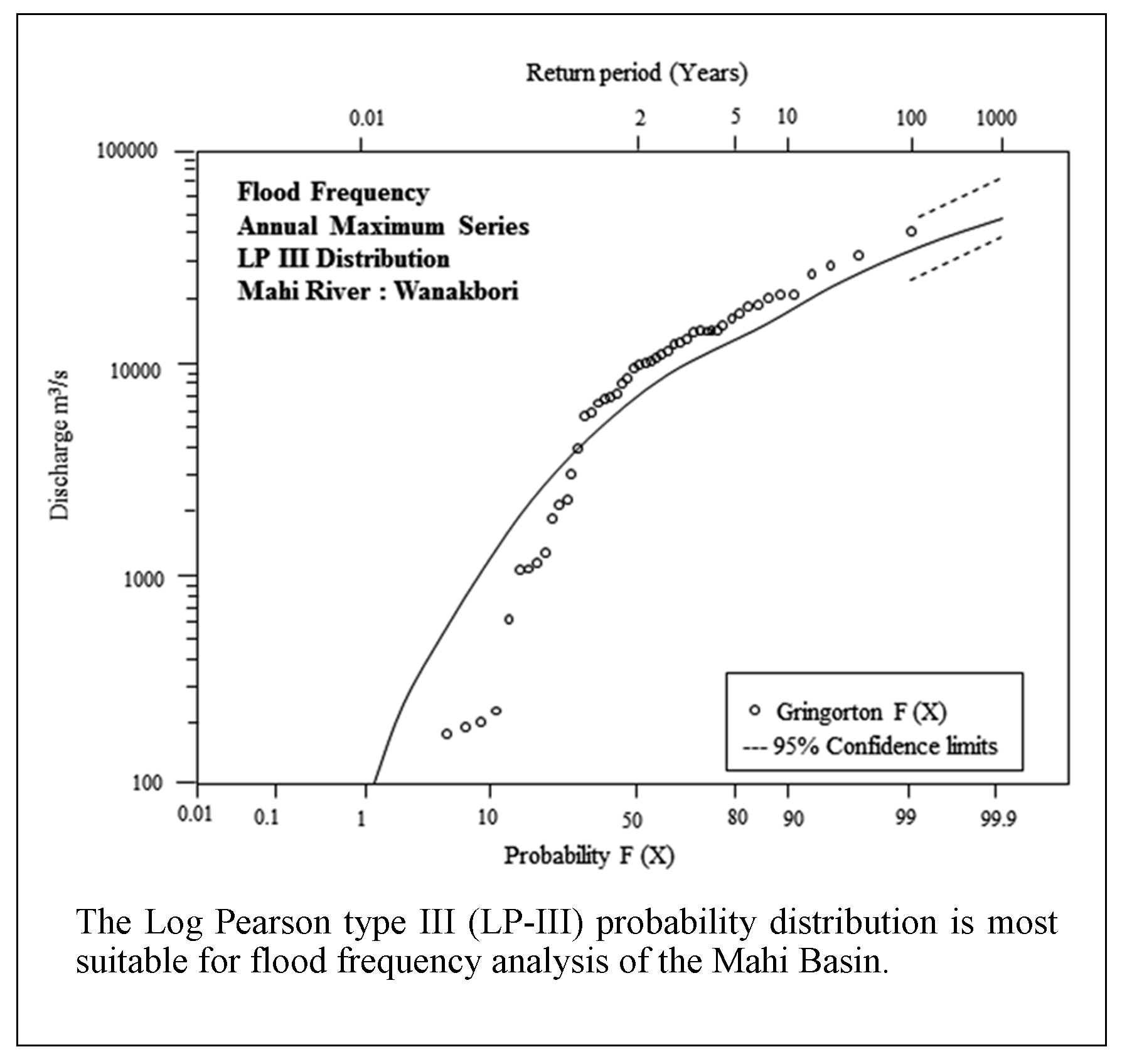
The Log Pearson type III (LP-III) probability distribution is most suitable for flood frequency analysis of the Mahi Basin.
The magnitude frequency analysis shows that the fitted lines are fairly close to the most of the data points.
The return period of the Qm, Qlf and Qmax seems to be very reliable.
The estimation of the discharges for the 100-yr flood is close to the observed Qmax discharge.
Abstract
Flood frequency analysis is one of the techniques of examination of peak stream flow frequency and magnitude in the field of flood hydrology, flood geomorphology and hydraulic engineering. In the present study, Log Pearson Type III (LP-III) probability distribution has applied for flood series data of four sites on the Mahi River namely Mataji, Paderdi Badi, Wanakbori and Khanpur and of three sites on its tributaries such as Anas at Chakaliya, Som at Rangeli and Jakham at Dhariawad. The annual maximum series data for the record length of 26-51 years have been used for the present study. The time series plots of the data indicate that two largest ever recorded floods were observed in the year 1973 and 2006 on the Mahi River. The estimated discharges of 100 year return period range between 3676 m3/s and 47632 m3/s. The return period of the largest ever recorded flood on the Mahi River at Wankbori (40663 m3/s) is 127-yr. The recurrence interval of mean annual discharges (Qm) is between 2.73-yr and 3.95-yr, whereas, the return period of large floods (Qlf) range from 6.24-yr to 9.33-yr. The magnitude-frequency analysis curves represent the reliable estimates of the high floods. The fitted lines are fairly close to the most of the data points. Therefore, it can be reliably and conveniently used to read the recurrence intervals for a given magnitude and vice versa.
Keywords
Annual Maximum Series , return period , peak discharge , Log Pearson Type III , Flood frequency analysis
1 . INTRODUCTION
Flood frequency analysis is one of the most commonly used techniques by the hydrologists, geomorphologists and hydraulic engineers to estimate the recurrence interval of peak discharge for a given site and is displayed as a flood frequency curve. However, availability of the longest flood series data along with the historic pre-instrumental records are required for the higher accuracy in the estimation of discharges for various return periods (Cunnane, 1989; Merz and Bloschl, 2008a; Merz and Bloschl, 2008b; Gaal et al., 2010 and Elleder et al., 2013). Brazdil et al. (2006) studied historic hydrological materials to estimate floods threat in Europe. There are several flood probability distribution models such as the generalized extreme value, Gumbel extreme value type I (GEVI), Log-Normal, Log Pearson type III (LP-III) to enumerate the magnitude and return period of floods, none of them gained universally recognition and unambiguous for a country (Law and Tasker, 2003). Foster (1924) introduced the Log Pearson Type III (LP-III) frequency distribution for describing the flood data. Griffis and Stendinger (2007, 2009), Phien and Jivajirajah (1984) used LP-III distribution to estimate maximum annual rainfall and discharges. Millington et al. (2011) estimated discharges for different return periods by comparing GEV, LP-III and Gumbel probability distribution. A frequency factor based method in flood frequency analysis for random generation of five distributions (Normal, Lognormal, Extreme Value Type I, Pearson Type III and Log Pearson Type III) was presented by Cheng et al. (2007).
Chow et al. (1988) stated that a curve produced by the flood frequency analysis have been used in the design of the hydraulic structures. Srikanthan and McMahon (1981) and McMahon and Srikanthan (1981) examined the applicability of LP-III distribution to Australian rivers. Singo et al. (2013) suggested that the Log Pearson Type III is the best fit probability model for flood prone Luvuvhu Basin of South Africa. Shen et al., (1980) compared the results of the Log Pearson type III and Gumbel distributions and opine that LP-III distribution is a better description of field data. The United State Water Resources Council (USWRC) in 1967 has recommended Log Pearson Type III (LP-III) probability distribution and subsequently updated in 1975, 1977 and 1981 as the base method of flood frequency analysis in the United States. It has been commonly applied in many parts of the world. Besides, the Institute of Engineers Australia (1987) also recommended that LP-III distribution be fitted to annual peak discharge data by using mean, standard deviation and coefficient of skewness of the logarithms of flow data (Pilgrim, 1987; Kottegoda and Rosso, 1997; Koutrouvelis and Canavos, 2000).
The Normal, Lognormal, Gumbel extreme value and Log Pearson type III probability distributions have been adopted to find flood frequency for different return periods by Jha and Bairagya, (2011) and Kumar et al., (2003) for deltaic region and Middle subzone 1(f) of Ganga Basin respectively. Hire and Patil, (2018) stated that GEVI probability distribution is best fit for the bedrock Par River in the western India. Bedrock channel morphology of the Par River shows high spatial variability in terms of flood hydraulics and hydrodynamics (Patil el al., 2017). Besides, Hire, (2000) also studied the flood frequency characteristics of the Tapi River by comparing Gumbel Extreme Value Type I and LP-III probability distributions. In case of Indian rivers, analysis reveals that LP-III distribution gives consistent results for estimating peak discharges up to 100-yr recurrence interval (Sakthivadivel and Raghupathy, 1978). Therefore, in view of the basin size and meteorological characteristics of the Mahi Basin Log Pearson type III (LP-III) probability distribution has been applied to the annual maximum series (AMS) data.
2 . STUDY AREA
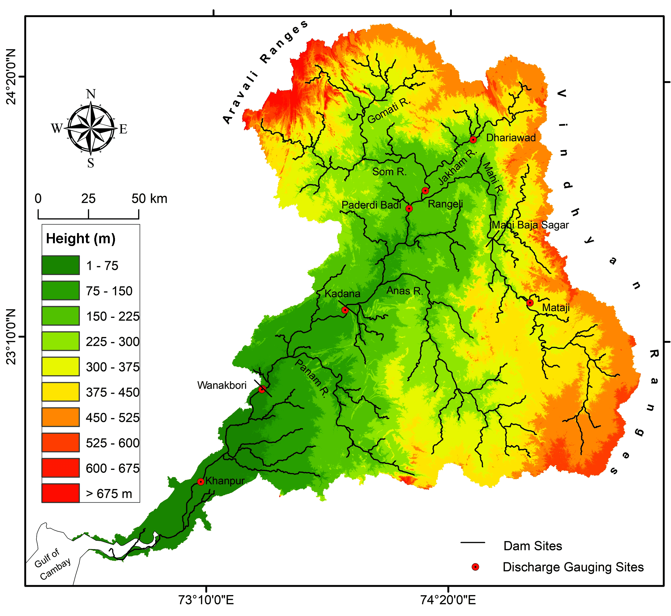
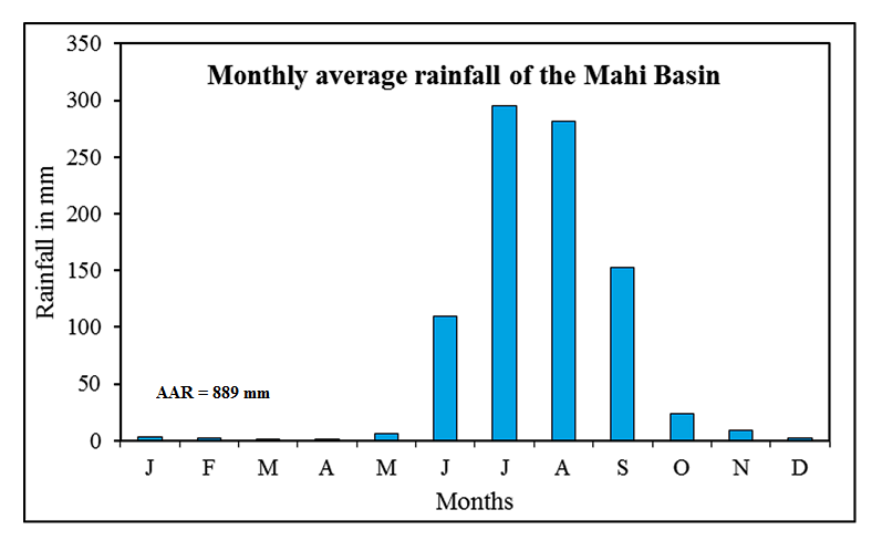
The Mahi River originates from Malwa Plateau near the village Mindha in Sardarpur tehsil in Dhar district of Madhya Pradesh at an elevation of 500 m above ASL. It lies between 72°21ʹ to 75°19ʹ E longitudes and 21°46ʹ to 24°30ʹ N latitudes. It is bounded by Aravalli hills on the north and the northwest, by Malwa Plateau on the east, by the Vindhyas on the south and by the Gulf of Khambhat on the west (Figure 1). It drains through states of Madhya Pradesh, Rajasthan and Gujarat for a total length of 583 km. The Mahi Basin has total catchment area of 34,842 km2. The Som is its principal tributary which joins from right, and the Anas and the Panam join the river from left. The average annual rainfall (AAR) of the basin is 889 mm. The southwest monsoon sets in by the middle of June and withdraws by the first week of October. The Mahi Basin receives 97 percent of total rainfall during the monsoon months of which 45% is received in July and August (Figure 2). The rainfall is mainly influenced by the southwest monsoon.
Figure 1. Physiography of the Mahi Basin and discharge gauging sites
Figure 2. Monthly average rainfall of the Mahi Basin
3 . DATA AND METHODOLOGY
Annual Maximum Series (AMS) data have been obtained from Central Water Commission (CWC) for the analysis of magnitude and frequency of floods on the Mahi River and its tributaries. The data have been made available for four sites on the Mahi namely, Mataji, Paderdi Badi, Wanakbori and Khanpur and three sites on its tributaries such as Som at Rangeli, Jakham at Dhariawad and Anas at Chakaliya (Figure 1). The data record length for these sites ranges between 26 and 51 years (Table 1).
Table 1. Hydro-geomorphic parameters of the Mahi River and its tributaries
River
Site
Record length (Years)
Elevation of the site (m)
Upstream Area (km2)
Qmax m3/s (Years)
Mahi
Mataji
1982 – 2016 (35)
292
3880
8075 (2005)
Mahi
Paderdi Badi
1978 – 2016 (39)
133
16247
16153 (2006)
Mahi
Wanakbori
1959 – 2009 (51)
52
30665
40663 (1973)
Mahi
Khanpur
1979 – 2016 (38)
11
32510
31062 (2006)
Anas
Chakaliya
1991 – 2016 (26)
219
3121
6956 (2005)
Som
Rangeli
1978 – 2016 (39)
148
8329
5179 (2006)
Jakham
Dhariawad
1990 – 2016 (37)
222
1510
1980 (2006)
Source: Central Water Commission (CWC).
The fitting the distribution needs of computing the mean (Qm), standard deviation (σ), and coefficient of skewness (Cs), of the logarithms of the annual peak-flow record in order to describe the mid-point, slope and curvature of the magnitude frequency curve respectively. Therefore, annual maximum discharge data have been analyzed by applying basic statistical techniques. Besides, time series graph of annual peak discharges for all the stations have been derived for better understanding of spatio-temporal variations in the peak flood discharges.
The expected design flood discharges have been calculated for return periods of 2, 5, 10, 25, 50 and 100 yrs. When three-parameter gamma distribution is used to the logs (either to the base of 10 or natural) of the AMS data, it is called the LP-III distribution (Bedient and Huber, 1989). The discharges of given recurrence intervals were estimated with the help of following equation (equation (1)) (Viessman et al., 1989)
where, log QT is log of discharge of required return period, Qm log Q is mean of log of AMS, σ log Q is standard deviation of log of AMS, and K(T) = frequency factor of return period (T). K (T) value is based on skewness coefficient of log of AMS data. The K (T) values were obtained from tables given in the books on Hydrology (Raghunath, 2006).
The recurrence interval of given discharges are often estimated graphically or with the help of table of frequency factor (K) (Bedient and Huber, 1989). The recurrence interval of preferred discharges such as Qm, Qlf and Qmax were calculated mathematically. Where, Qm is the mean annual peak discharge, Qlf is the large flood ((All floods that exceeds mean plus one standard deviation (>Qm+1σ)) and Qmax is the observed peak discharge on record (Hire, 2000).
The frequency distribution has been shown graphically on lognormal probability paper by plotting probability against the values of discharge for assured recurrence interval by using (equation (1)). Several formulae have been used to calculate plotting positions, however, of the several formulae in use, the best is due to Gringorten since the outliers fall into line better than other plotting positions (Shaw, 1988). The F(X) values have been calculated as follows (equation (2));
The 95% confidence limits have been placed on frequency curves. A method proposed by Beard (1975) has been adopted to form a reliability band of the confidence limit.
4 . RESULT AND DISCUSSION
4.1 Annual Flood Series Analysis
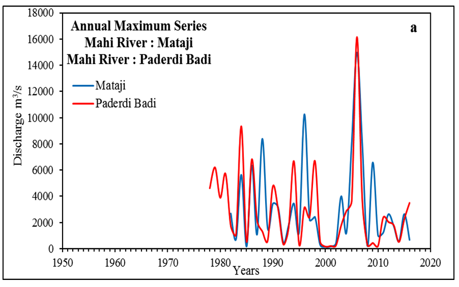
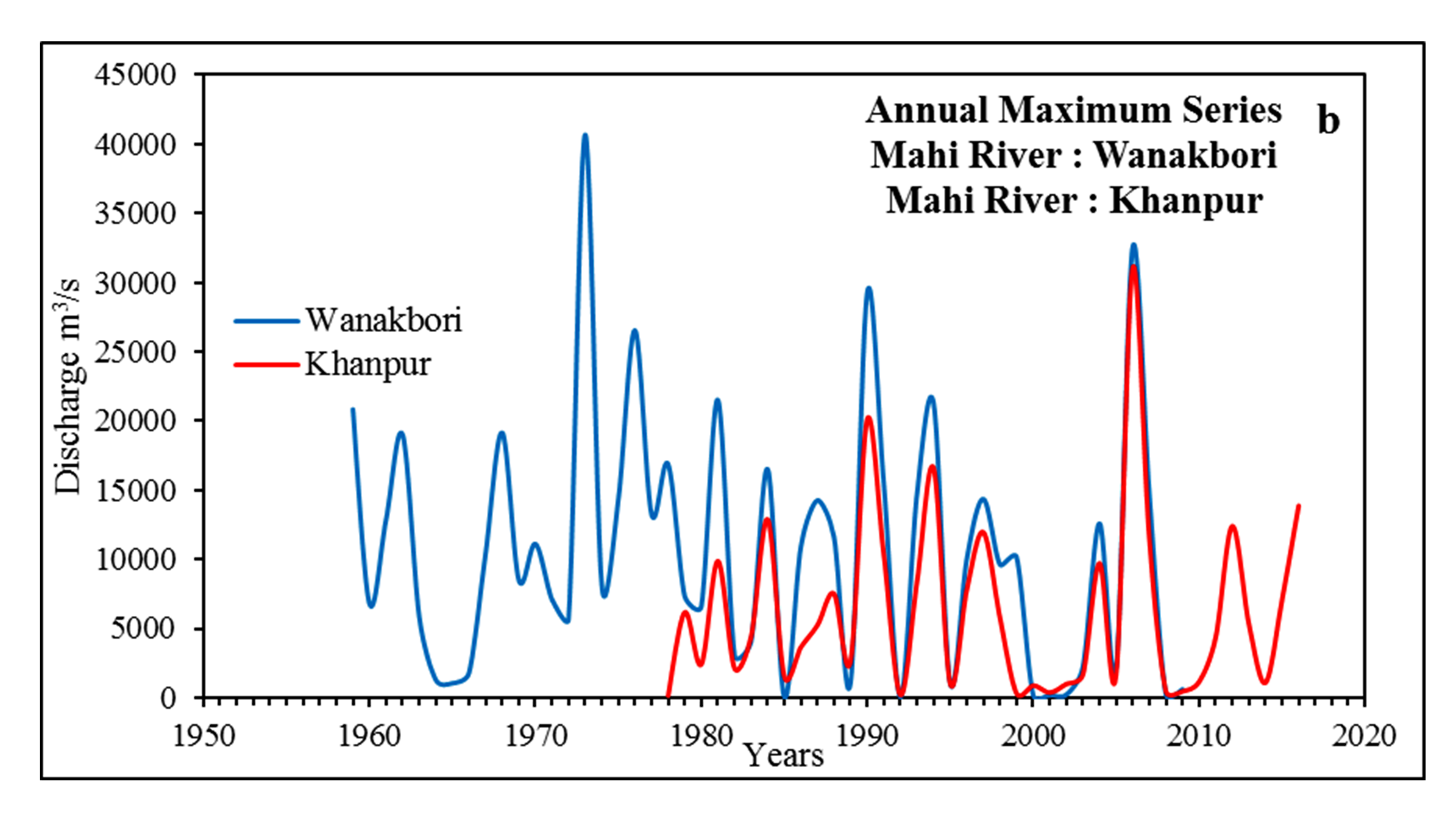
According to Ward (1978) the maximum peak flow recorded in every single year for successions of years at a gauging site is measured as annual maximum series (AMS). The analysis of such annual flood series (AMS) has great significance in the flood hydrology research. Although the aim of the research is flood frequency analysis, time series graph of annual peak discharge for all the site are shown in Figure 3a, 3b and 3c. The time series plot of Wanakbori indicates that two largest floods were observed in the year 1973 and 2006 with discharge 40663 m3/s and 32557 m3/s respectively. In addition to this, in the year 1994 and 2006, the Mahi Basin experienced major floods after the year 1973 and 1976.
Figure 3a. Annual maximum series, Mahi River at Mataji and Paderdi Badi
Figure 3b. Annual maximum series, Mahi River at Wanakbori and Khanpur
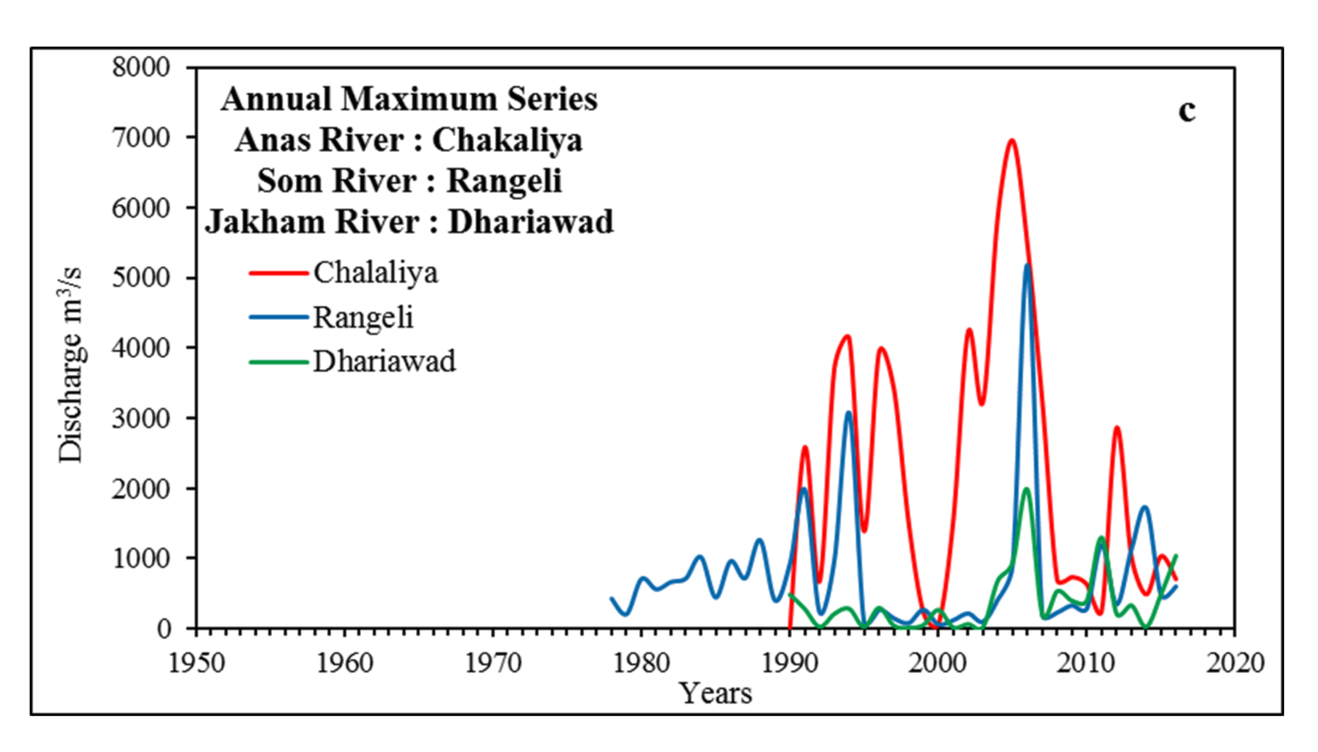
Figure 3c. Annual maximum series, Anas River at Chakaliya, Som River at Rangeli and Jakham River at Dhariawad
4.2 Estimation of Discharges for Return Periods
A designed flood has been determined on the basis of observed Qmax or historic flood. Therefore, the continuous, long and good quality of record of stream discharges is essential for the more accurate appraisal of recurrence interval of the peak flows. Generally, the AMS data have been more recurrently applied for the analyses. Accordingly, peak flows have been estimated for different return periods such as 2, 5, 10, 25, 50, and 100 yrs. by using Log Pearson type III (LP-III) probability distribution and the estimated discharges are given in (Table 2).
Table 2. Estimated discharges in m3/s for different return periods for different gauging sites on the Mahi River and its tributaries (Based on LP-III distribution)
River
Site
Record
length
Estimated Discharges (m3/s)
2 Yr.
5 Yr.
10 Yr.
25 Yr.
50 Yr.
100 Yr.
Mahi
Mataji
35
1748
4672
7464
11910
15823
20174
Mahi
Paderdi Badi
39
1772
4681
7437
11800
15623
19861
Mahi
Wanakbori
51
7329
20723
29641
38784
43873
47632
Mahi
Khanpur
38
3624
10352
16644
26211
34193
42672
Anas
Chakaliya
26
1940
4094
4873
5335
5479
5544
Som
Rangeli
39
450
1074
1708
2823
3920
5283
Jakham
Dhariawad
27
194
632
1111
1949
2744
3676
The highest (47632 m3/s) estimated discharge of 100 year return period was for the Wanakbori site on the Mahi River in the Gujarat state. However, the peak discharge of 40663 m3/s magnitude was observed on the Mahi River in the year 1973 generated by heavy to very heavy rainfall due to the low pressure system that crossed the Mahi Basin and centered at Modasa in the Sabarmati Basin adjacent to the Mahi Basin. The minimum estimated discharge is 19861 m3/s for 100 year return period on the Mahi River is for the Paderdi Badi site. Besides, the lowest estimated discharges are observed in case of the Jakham River at Dhariawad which is a tributary of the Som River. This is attributed to less annual rainfall in the upper catchment of the river and controlled discharge due to construction of the Jakham Dam.
The estimation of the discharges for different return period has significance in the flood geomorphology, flood hydrology and hydraulic engineering while designing hydraulic structures such as bridges and dams. Therefore, accuracy in the estimation of design flood based on long history of flood is essential. For example, as stated by More (1986), at the time of construction of Kadana Dam on the Mahi River, the data about peak discharge (Qmax) of the large flood of 1927 was not available to estimate the accurate design flood of the Kadana Dam. Therefore, the original project estimate provided for a maximum flood of 23096 m3/s. The design flood was revised with the magnitude 31087 m3/s at the time of project clearance in 1966, with 19 spillway gates. However, due to the flood of 1968 with the observed discharge of magnitude 21820 m3/s, the design flood was further revised to 36840 m3/s and for this revised flood, 21 spillway gates including one standby were provided. During 1973 due to heavy to very heavy rainfall associated with the low pressure system (LPS), unprecedented flood of the magnitude 32986 m3/s was observed which again forced to revise design flood of Kadana dam and finally maximum probable flood with the magnitude 46871 m3/s was considered in March 1974. To account for this flood the additional spillway is located 2 km away from main spillway on the right bank in the saddle. This example, therefore, suggests the significance of record length and flood frequency analysis for construction of bridges and dams. Therefore, application of flood frequency analysis is inevitable.
4.3 Estimation of Return Period
The estimation of return period is of the great significance for the safety of hydraulic structures. Therefore, an attempt has been made to find out the return period of mean annual peak discharge (Qm), large flood (Qlf) and actually observed maximum annual peak discharge (Qmax) by applying the Log Pearson type III distribution and result have been shown in (Table 3).
Table 3. Return period of Qm, Qlf and Qmax for different sites on the Mahi River and its tributaries (Based on Log Pearson type III)
River
Site
Record
length
Q m3/s
Return period (yr)
Mahi
Mataji
35
Qm = 3135
3.56
Qlf = 6568
7.76
Qmax = 14972
36.80
Mahi
Paderdi Badi
39
Qm = 2968
3.59
Qlf = 6132
9.33
Qmax = 16153
57.00
Mahi
Wanakbori
51
Qm = 10587
3.95
Qlf = 19757
8.27
Qmax = 40663
126.56
Mahi
Khanpur
38
Qm = 6448
3.65
Qlf = 13022
7.42
Qmax = 31062
67.41
Anas
Chakaliya
26
Qm = 2329
2.73
Qlf = 4275
6.24
Qmax = 6956
101
Som
Rangeli
39
Qm = 753
4.43
Qlf = 1697
6.47
Qmax = 5179
104.68
Jakham
Dhariawad
27
Qm = 392
2.74
Qlf = 853
7.59
Qmax = 1980
81.97
The recurrence interval of Qm is between 2.73-yr and 3.95-yr, whereas, the return period of Qlf ranges from 6.24-yr to 9.33-yr. The magnitude-frequency analysis reveals high return period (127-yr) for the Qmax (40663 m3/s) recorded at Wanakbori site in the year 1973. Moreover, the return periods of Qmax for all the sites on the tributaries of the Mahi River also shows high recurrence interval as compared to other sites on the Mahi River. The estimates based LP-III indicate that large floods are likely to occur once in 6 to 9 years.
4.4 Magnitude Frequency Curve
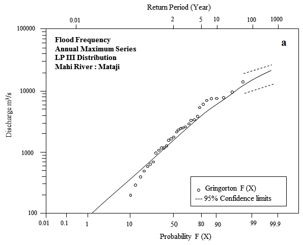
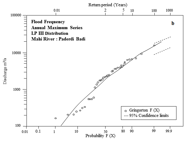
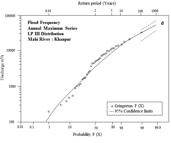
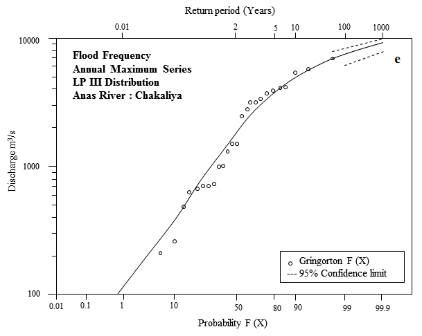
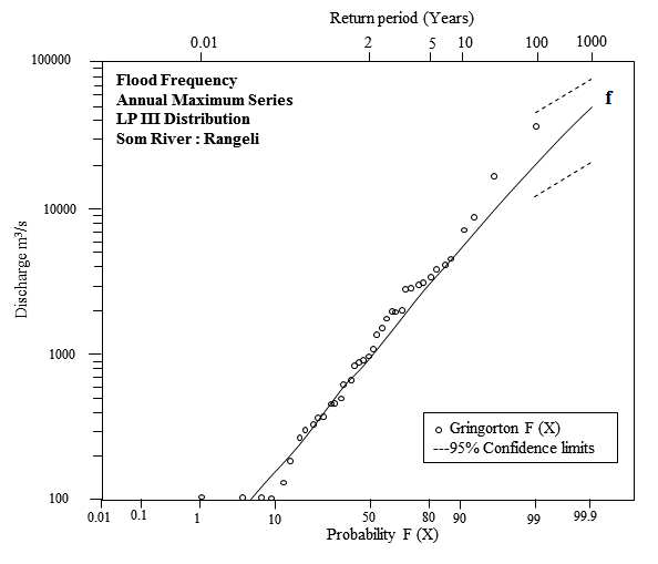
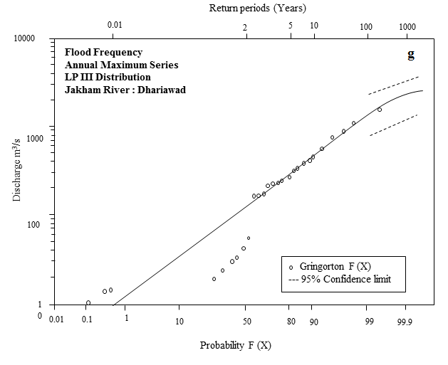
The magnitude-frequency analysis graphs of the Log Pearson type III (Figure 4) show that the fitted lines are fairly close to the most of the data points and, therefore, can be reliably and conveniently used to read the recurrence intervals for a given magnitude and vice versa. The graphs also indicate that the return periods of Qmax of different stations predicted by LP-III distribution are likely to be quite reliable. However, extrapolation of the lines to estimate the discharges for a higher recurrence interval (200-yr, 500-yr or 1000-yr) is not likely to be accurate and reliable due to short record length.
Figure 4a. Flood frequency, annual maximum series, LP III distribution, Mahi River: Mataji
Figure 4b. Flood frequency, annual maximum series, LP III distribution, Mahi River: Paderdi Badi
Figure 4c. Flood frequency, annual maximum series, LP III distribution, Mahi River: Wanakbori
Figure 4d. Flood frequency, annual maximum series, LP III distribution, Mahi River: Khanpur
Figure 4e. Flood frequency, annual maximum series, LP III distribution, Anas River: Chakaliya
Figure 4f. Flood frequency, annual maximum series, LP III distribution, Som River: Rangeli
Figure 4g. Flood frequency, annual maximum series, LP III distribution, Jakham River: Dhariawad
5 . CONCLUSIONS
The LP-III analysis shows estimated discharges for low recurrence interval are close to the observed peak discharges and return period of the mean annual flood (Qm), large floods (Qlf) and peak flood (Qmax) also fairly reliable. Besides, the value of design flood (46871 m3/s) of the Kadana Dam and estimated discharge (47632 m3/s) of 100-yr return period for Wanakbori site (downstream of Kadana Dam) based on the flood of 1973 are perfectly matching. Flood frequency fitted lines are fairly close to the data points indicate the best fit to annual maximum series of the river under review. Therefore, based on the observations it is said that the LP-III distribution is most suitable for flood frequency analysis of the Mahi River and its tributaries.
Tables
Figures
Conflict of Interest
The authors declare no conflict of interest.
Acknowledgements
Pramodkumar Hire is grateful to Science and Engineering Research Board, Department of Science and Technology, Government of India for financial support to conduct this research work (Project Number: EMR/2016/002590 dated February 21, 2017). The authors are thankful to Professor Vishwas S. Kale for his helpful and constructive comments and suggestions. Authors are grateful to Dr. Patil Archana for preparation of the Mahi Basin maps as well as for assistance in fieldwork and Dr. Rajendra Gunjal, Ms. Gitanjali Bramhankar for their support in data collection and in the field.
References
1.
Bedient, P. B. and Huber, W.C., 1989. Hydrology and Floodplain Analysis. Addison Wesley Publication Company, New York.
2.
Beard, L. R., 1975. Generalized evaluation of flash-flood potential. Technical Report - University of Texas. Austin, Central Research Water Resource. CRWR-124, 1-27.
Chow, V. T., Maidment, D. R. and Mays, L.W., 1988. Applied Hydrology, McGraw Hill, New York.
6.
Cunnane, C., 1989. Statistical distributions for flood-frequency analysis, World Meteorological Organization, Operational Hydrology Report No. 33 Secretariat of the World Meteorological Organization–No. 718, 61 p. plus appendixes.
Foster, H. A., 1924. Theoretical frequency curves and their application to engineering problems. Trans American Society of Civil Engineers, 87 (1), 142-173.
Jha, V. C. and Bairagya, H., 2011. Environmental impact of flood and their sustainable management in deltaic region of West Bengal, India. Caminhos de Geografia, 12 (39), 283-296.
Millington, N., Das, S. and Simonovic, S. P., 2011. The Comparison of GEV, Log-Pearson Type 3 and Gumbel Distributions in the Upper Thames River Watershed under Global Climate Models. Water Resources Research Report, 077, 10-19.
21.
More, D. K., 1986. Flood Control Operation of Kadana Reservoir. Master of Engineering in Hydrology, University of Roorkee, Roorkee (India).
22.
Kottegoda, N. T. and Rosso, R., 1997. Statistics, Probability, and Reliability for Civil and Environmental Engineers, McGraw Hill, New York.
Raghunath, H. M., 2006. Hydrology: principles, analysis and design. Second revised edition.
28.
Sakthivadivel, R. and Raghupathy, A., 1978. Frequency analysis of floods in some Indian rivers. Hydrology Review, 4, 57-67.
29.
Shaw, E. M., 1994. Hydrology in Practice. Taylor & Francis e-Library, 2005.
30.
Shen, H. W., Brvson, M. C. and Ochoa, I. D., 1980. Effect of tail behavior assumptions on flood predictions. Water Resource Research, 16, 361-364.
31.
Singo, L. R., Kundu, P. M., Odiyo, J. O., Mathivha, F. I. and Nkuna, T.R., 2013. Flood frequency analysis of annual maximum stream flows for Luvuvhu river catchment, Limpopo province, South Africa. University of Venda, Department of Hydrology and Water Resources, Thohoyandou, South Africa, 1-9.
32.
Srikanthan, R. and McMahon, T. A., 1981. Log Pearson III distribution -an empirically derived plotting position. Journal of Hydrology, 52,161-163.
33.
Viessman, W., Lewis, G. L. and Knapp, J. W., 1989. Introduction to Hydrology. Happer and Row Publishers, Singapore.
34.
Ward, R., 1978. Floods. A Geographical Perspective. The MacMillan Press Ltd., London.


 ,
Pramodkumar Hire 2
,
Pramodkumar Hire 2