Keywords

DEM , GIS , hydrology , Morphometric Aspects , Morphometric analysis , Watershed

1 . INTRODUCTION

Population pressure on water resources is increasing day by day in India. Watershed is fundamental unit for conservation and preservation of natural resources. Soil and water conservation are issues in watershed management. Water resource development plays role in economic and social development of any country (Nag, 1998; Reddy et al., 2004; Das and Mukherjee, 2005).

Morphometric analysis is the dimension and mathematical investigation of the Earth’s surface, shape, and measurement of the landforms (Clarke, 1966). It is easy to understand the behavior of the hydrological system (Agarwal, 1998) and assists in recognizing the hydrological distinctiveness and the results will be valuable input for comprehensive water resource management (Jawaharraj et al., 1998; Sree Devi et al., 2001). Horton (1940) and Strahler (1950) were initiated morphometric studies in the field of hydrology. The morphometric analysis involves the analysis of various linear, areal, and relief parameters of watershed. These parameters are very significant for watershed management and hydro-geomorphological investigation (Gaikwad ). The quantitative analysis of morphometric parameters is found to be of immense utility in river basin evolution, and it is very significant in understanding the landform processes, soil physical properties and erosion characteristics. They also reflect the quantity of erosion, waterlogging, flood, drought, etc. which significantly helpful to understand the rocks, climate, drainage, relief, and vegetation cover in the watershed.

Since the first quarter of 20^th century, drainage basin has been considered as areal unit of the geomorphic investigation, but as a basic geomorphic unit, these analyses useful for application of various morphometric techniques. The study of different properties of river basins becomes significant because of their consequence in the development of landform. Besides, it also provides essential input in the river basin development and understanding the hydrological properties. The present study performed to understand various morphometric aspects: linear, areal and relief of Kolavadi sub-watershed using geo-spatial techniques. Morphometric analysis using remote sensing and GIS techniques was widely used for watershed prioritization, sub-watershed analysis and management (Khan et al., 2001; Vittal et al., 2004; Chopra et al., 2005; Ratnam et al., 2005). GIS techniques have potentials of precise and timely spatial information for watershed planning and management.

2 . STUDY AREA

Kolavadi sub-watershed (10.66 sq.km) is situated between 18º 14ʹ 58" N to 18º 18ʹ 24" N and 73º 45ʹ 14" E to 73º 52ʹ 48" E (Figure 1). It is sub-watershed in upper Nira basin and lies in Western Ghats of Maharashtra. The revier has dendritic type of drainage pattern in the study area. The elevation ranges from 1040 to 620m above MSL. June to September are rainy months receive 973 mm average annual rainfall with July as the wettest month of the year.

Study area: Kolavadi sub-watershed

2.1           Geomorphology

The geomorphological characteristics are helpful to understand the hydrological behavior of the watershed and its effective management (Agarwal et al., 2011). Geomorphology of the Kolavadi sub-watershed as ascertained based on 1:50000 scale morphological maps (MRSAC, Nagpur) and remote sensing data. The northern part is mostly included in HDP-A (highly dissected plateau with exposed rock and negligible soil cover) and is not favourable for groundwater recharge. The central area represents MDP-A, (moderately dissected plateau with exposed rock and thin soil cover), which is also not favorable for groundwater recharge (Figure 2). The southern part is considered as MDP-C, (moderately dissected plateau with thick soil cover and thick weathered zone) which can favour of agricultural activity.

Figure 2. Geomorphology

2.2           Land Use / Land Cover

Land use / land cover (LULC) in the region affects the infiltrating rate which shows the relationship between surface characteristics and groundwater recharge potentials (Kazakis et al., 2015). In this study, LULC of Kolavadi sub-watershed was analysed using Landsat 8 OLI/TIRS data of February 8, 2016. The study area was classified into seven LULC categories viz. barren land, open land, forest area, scrubs and without scrubs and croping land (single cropped: Kharif crops and double cropped- kharif + rabi crops). Land with vegetation cover includes forests and scrublands show more infiltration rate (Figure 3). Dense forests are obsereved in Northern part of the sub-watershed whereas agriculture: Kharif and Rabi along with the streams.

Figure 3. Land use land cover

3 . MATERIALS AND METHODS

The degree of morphometric aspects: linear, aerial, and relief aspects of the watershed were analsysd (Horton, 1945; Miller, 1953; Schumm, 1956; Langbein, 1947; Smart and Surkan, 1967; Strahler 1968; Mueller, 1968). The morphometric analysis of the basin has been based on Survey of India (SOI) topographical maps (47F/15) and open series map (E43H15) at 1:50000 scale for delineation and digitization of drainage basin.  Geomorphology map obtained from Maharashtra Remote Sensing Applications Centre (MRSAC), Nagpur (1:50000 scale). The parameters of the drainage basin derived from stream length, number of streams, basin area, perimeter and basin length. The morphometric parameters were calculated using the formula suggested by Horton (1945); Miller (1953), Schumm (1956) and Strahler (1964) for Kolavadi sub-watersheds of Gunjavne River in Maharashtra (India).

The thematic maps were verified and modifid based on groundtrouth informatin collected using GPS and fieldwork techniques. Initially, the topographic maps were geo-referenced and stream network digitized in GIS environment. The stream ordering was carried out using Horton’s law. Linear aspects include stream order (U), stream number (Nu), stream length (Lu), bifurcation ratio (Rb), mean length of streams of corresponding orders (Lum), stream length ratio (Lur), and mean stream length ratio (Lurm). Areal aspects comprise basin area (A), basin perimeter (P), stream frequency (Fs), circularity ratio (Rc), elongation ratio (Re), form factor (Ff), length of overland flow (Lg), texture ratio (Rt), constant of channel maintenance (C) and drainage density (Dd). Relief aspects include basin relief (H), relief ratio (Rhl), relative relief (RR), ruggedness number (Rn), and slope analysis (m). All these parameters were computed and analyzed for the Kolavadi sub-watershed (Table 1).

4 . RESULTS AND DISCUSSIONS

4.1 Morphometric Analysis - Linear Aspects

The linear aspects of sub-watershed deliberate in terms of stream orders, associated with attributes of number and the average length of streams with their corresponding order. In the present study, various linear aspects including stream order (U), stream number (Nu), stream length (Lu), bifurcation ratio (Rb), stream length ratio (Lur), and mean stream length ratio (Lurm) were considered for detailed analysis (Table 2).

4.1.1 Stream Order (U)

‘Stream ordering’ is the primary step in quantitative analysis of watershed. It expresses the hierarchical relationship between stream segments, their connectivity and discharge arising from contributing catchments. In the beginning stage, the stream order concept proposed by Horton in 1945. Subsequently, this concept customized by Strahler (). According to Strahler (1980), the first-order streams are those who have no tributaries. The second-order streams are tributaries of first-order channels only. Second-order channels join to segments of third-order streams. Similarly, two third-order channels discharging water to fourth-order channels and so on. The trunk stream through which, total discharge of water and sediments pass is the stream segment of the highest order.

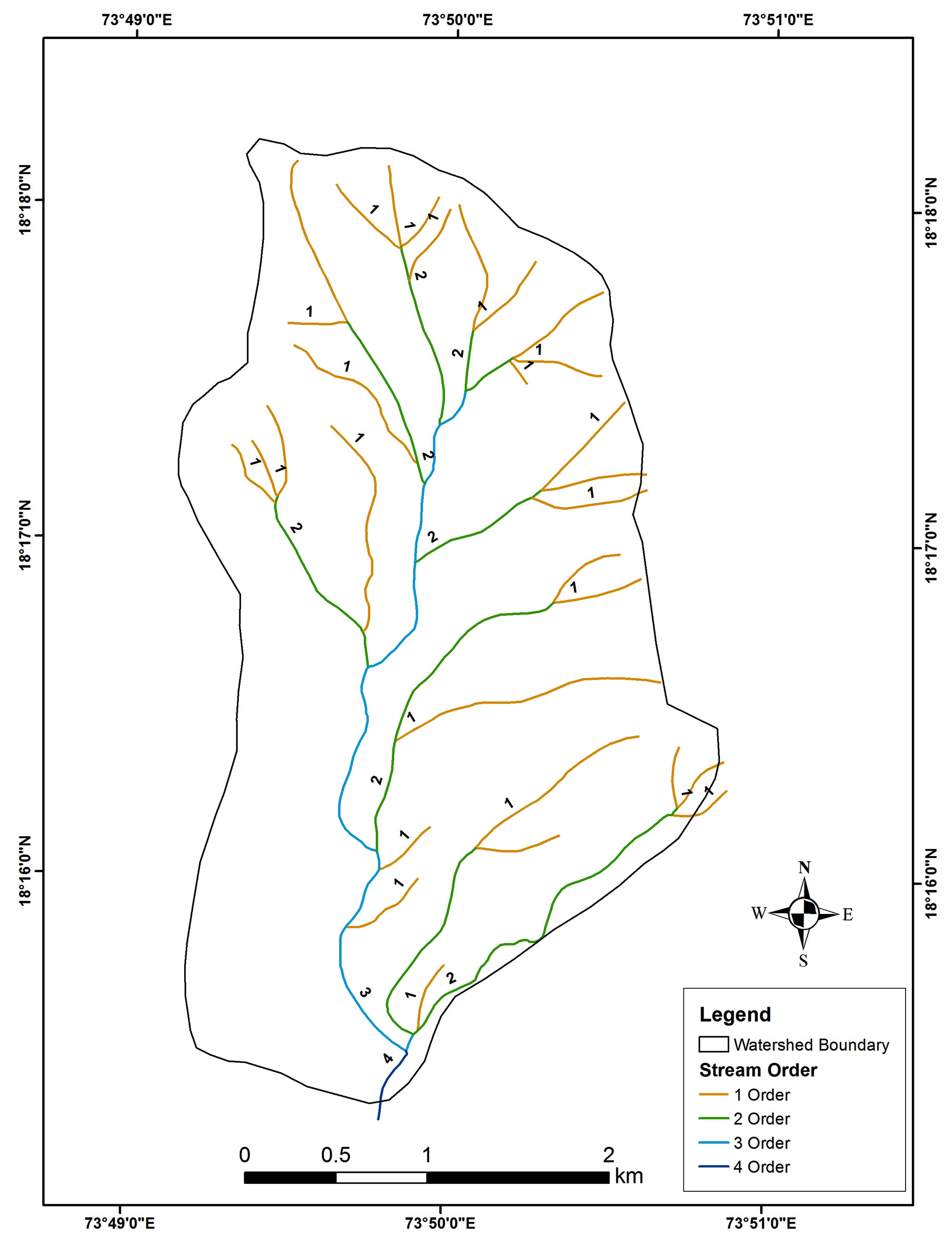
In the present study, the stream ordering is based on the method proposed by Strahler (1980) and is a 4^th order stream network. The maximum frequency is in case of first-order streams and reducing as stream order increases. About 42 streams observed in Kolavadi sub-watershed, out of that 30 are first order, 9 are second order, 2 are third order, and only one stream in fourth order (Figure 4). Drainage pattern of Kolavadi sub-watershed is dendritic (tree-shaped) type indicates homogeneity in texture without structural control.

Figure 4. Stream orders

4.1.2 Stream Number (Nu)

The ‘numbers of stream segments of each order form an inverse geometric sequence with an order number’ (Horton, 1945). About 42 streams observed in Kolavadi sub-watershed. The maximum frequency was in case of the first-order streams and decreases as the stream-order increases.

4.1.3 Stream Length (Lu)

Stream length reveals the surface runoff characteristics of the basin. It has been measured with the help of rotameter. The stream of relatively smaller length is characteristic of areas with more extensive slopes and exquisite surface. In general, ‘the total length of stream segments is maximum in the first-order streams’ and decreases with increasing stream orders. Horton’s law of stream length suggests a geometric relationship between the number of stream segments in successive stream orders and landforms (Horton, 1945). In the present study, stream length has calculated by using the Survey of India (SOI) topographic maps.

The maximum total length of streams is observed for first-order streams (Table 2) and decreases as the order increases. First-order streams are of 17.56km length, second-order streams are 11.84km, third-order streams are 5.16km and fourth-order stream is 0.42km long. This inconsistency is probably due to variation in relief, lithological variation and rock condition over the area (Singh, 1997).

4.1.4 Mean Stream Length (Lum)

The mean stream length is a dimensionless property show size of the drainage network and basin surfaces () mean stream length (Lum) is ratio between total stream length and number of streams (by order). The mean stream length of the study area is 0.59 for first order, 1.32 for the second order, 2.58 for the and 0.42 for . The mean stream length increases with increasing stream orders .

4.1.5 Stream Length Ratio (Lur)

‘Stream length ratio’ is the ratio between ‘mean length of stream’ of selected order and total stream segments in next order (Horton, 1945). The variations in stream length ratio between streams of different order indicate late youth stage of geomorphic development (Singh and Singh, 1997). The stream length ratio in the study area varies from 0.16 to 2.25.

4.1.6 Bifurcation Ratio (Rb)

Bifurcation ratio is ratio of total number of streams for selected order with total streams of next higher order in the drainage basin. It is an index of relief and dissection (Horton, 1945; Schumm, 1956). Bifurcation ratio shows the degree of integration between the streams of different orders in a drainage basin. The lesser values show flatness or rolling physiography of the basin while the higher values indicate robust structural control on drainage pattern with well-dissected drainage basins (Strahler, 1980).

Total and mean bifurcation ratios of the Kolavadi sub-watershed are 9.83 and 3.27, respectively. characteristically varies between 3 and 5 for the

4.2 Morphometric Analysis - Areal Aspects

Areal aspects include drainage density, stream frequency, texture ratio, form factors, circulatory ratio, elongation ratio, length of overland flow and the constant of channel maintenance. This analysis can be useful to establish a relationship between the stream discharge and the total area of the basin.

4.2.1 Basin Area (A)

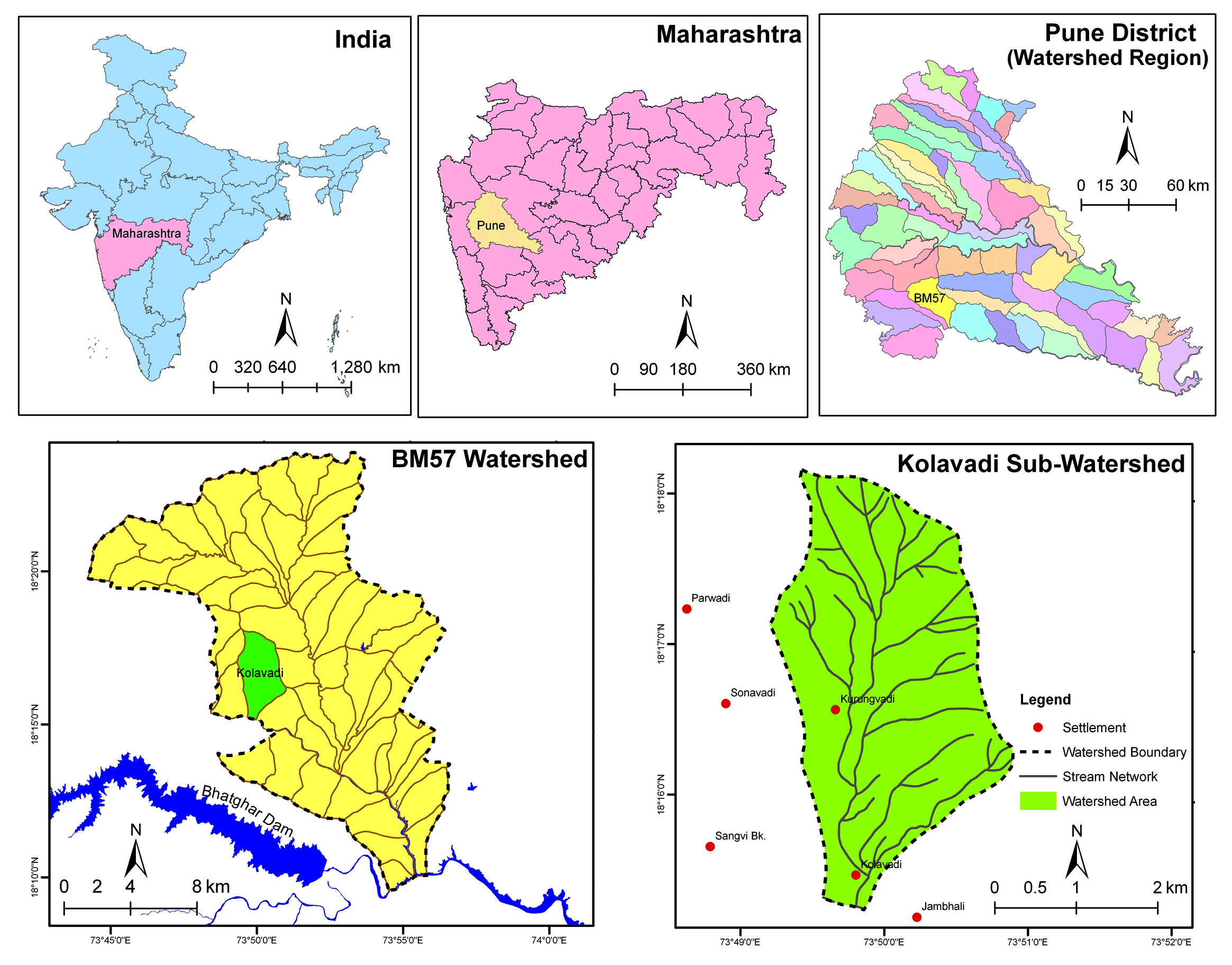
The total area of the basin is a significant parameter in morphometric analysis. The shape of a basin originates as a pear and over the course tends to get more elongated in nature. The area of the Kolavadi sub-watershed is 10.66 sq. km.

4.2.2 Basin Perimeter (P)

The external boundary of the watershed enclosed the total area. The length of this external boundary which also is measured along the water divide is the basin perimeter. Perimeter is indicators of watershed size and shape (Schumm, 1956). The perimeter of the Kolavadi sub-watershed is 14.18km.

4.2.3 Basin Length (Lb)

The basin length is the straight linear distance from the mouth of the basin to the farthest point on the water divide. This line intersects the projection of the direction of the line from the source of the mainstream (Horton, 1932). The length of the sub-watershed of Kolavadi is 5.1km.

4.2.4 Length Area Relation (Lar)

According to Hack, the stream length and basin area are related by simple power functions in large number of basins (Hack, 1957). The length area relation of the Kolavadi sub-watershed is 8.95.

4.2.5 Lemniscate’s Value (k)

The slope of the basin can be expressed with the use of Lemniscate’s value (Chorley, 1957). The Lemniscate’s (k) value for the Kolavadi sub-watershed being 2.44, indicates that the basin occupied by a large number of streams in the higher order.

4.2.6 Drainage Density (Dd)

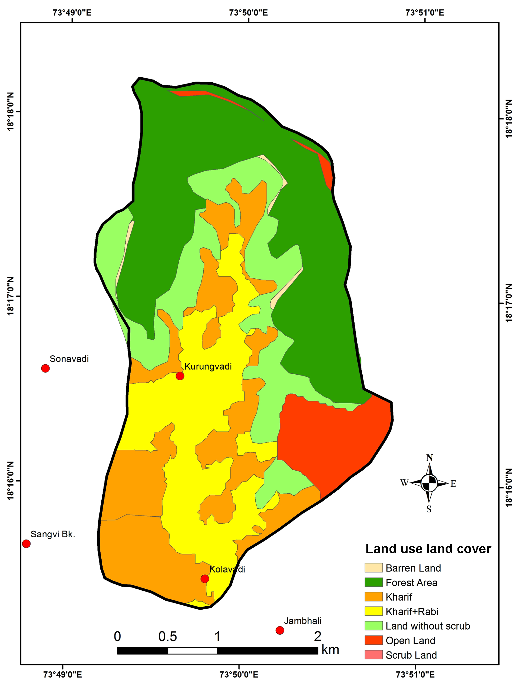
The ratio of the ‘total length of streams of all orders’ to ‘area’ of the basin is defined as drainage density and is expressed in km/km². The closeness in the spacing of channels can be identified vide the use of drainage density. This is helpful for quantitative measures of average length of the a stream to the whole basin. It is classified into 5 different classes: very coarse (<1.2), low (1.2 to 2.4), moderate (2.4 to 3.6), high (3.6 to 4.8) and very high (4.6 to 6). Higher values are indicative of lower permiability, sparse vegetation, and rugged relief and lower values are indicative of higher permiability (Strahler, 1964). The drainage density in the Kolavadi sub-watershed is about 3.28 km/km2, which is a moderate and indicative of highly permeable subsoil and vegetation cover (Nag, 1998).

4.2.7 Stream Frequency (Fs)

Expression of the total number of stream segments belonging to all orders per unit area is identified as stream frequency (Horton, 1932). Stream frequency tends to be in positive correlation with drainage density. The stream frequency of the study area is 3.94. A higher value of stream frequency indicates at a faster runoff and flooding in the catchment (Kale and Gupta, 2001).

4.2.8 Texture Ratio (Rt)

The ratio between the numbers of first-order streams to the basin perimeter can be defined as the texture ratio (Chorley, 1957). It is indicative of the spacing of streams. Smith (1939) derived a five fold classification from very coarse texture (<2), through coarse texture (2 to 4), moderate texture (4 to 6), fine texture (6 to 8) to very fine texture (>8) classes. The drainage texture of the Kolavadi sub-watershed is 2.96 and indicative of a coarse drainage texture.

4.2.9 Form Factor (Ff)

Form factor (Ff) is the ratio between the basin area and the source of the basin length. The flow intensity of a unit area can be identified vide this factor (Horton, 1945). Circular shaped watershed have a lower value of from factor (0.754) as against an elongated shape would have a value nearing zero and whilst a value of 1 would denote a perfectly circular shape. The form factor of the Kolavadi sub-watershed at 0.40 symbolizes a highly elongated shape and highly vulnerable to erosion.

4.2.10 Elongation Ratio (Re)

The shape or form of a basin can be identified through the elongation ratio. It is calculated as the ratio between the diameter of a circle having an area similar to the basin and the maximum basin length (Schumm, 1956). Varied climatic and geophysical environments are valued between the ratio values of 0.60 to 1.00. Values nearing 1.00 are indicative of a lower relief, while those between 0.60 and 0.80 can be associated with steep ground slopes of high relief (Strahler, 1964). The varying shapes of a watershed viz. circular shape (0.9- 0.10), oval (0.8-0.9), and less elongated (<0.7). The elongation ratio of Kolavadi sub-watershed is 0.72 indicative of a near elongated shape.

4.2.11 Circularity Ratio (Rc)

Miller (1953) defined circularity ratio is on similar grounds as elongation ratio where, it is the ratio of the basin area to the area of circle having a same circumference as the perimeter of the basin. This ratio is a dimensionless index used to identify the outline shape of the basin. The value varies from zero (a line) to one (a circle). The value tends to be influenced by length and frequency of streams in respective orders, gradient, lithology and pattern of drainage (Umrikar, 2016). Circularity ratio of the Kolavadi sub-watershed is 0.66, indicating a moderate shape of the basin. This implies a late youth stage of geomorphic development of the drainage basin.

4.2.12 Length of Overland Flow (Lg)

Horton (1945) identifies length of the water flow over the ground surface before concentrating in a stream channel. It is an independent variable affecting development of drainage basin. It can be equated to being half of the reciprocal value of drainage density. The length of overland flow in the Kolavadi sub-watershed is 6.56.

4.2.13 Constant of Channel Maintenance (km²/km) (C)

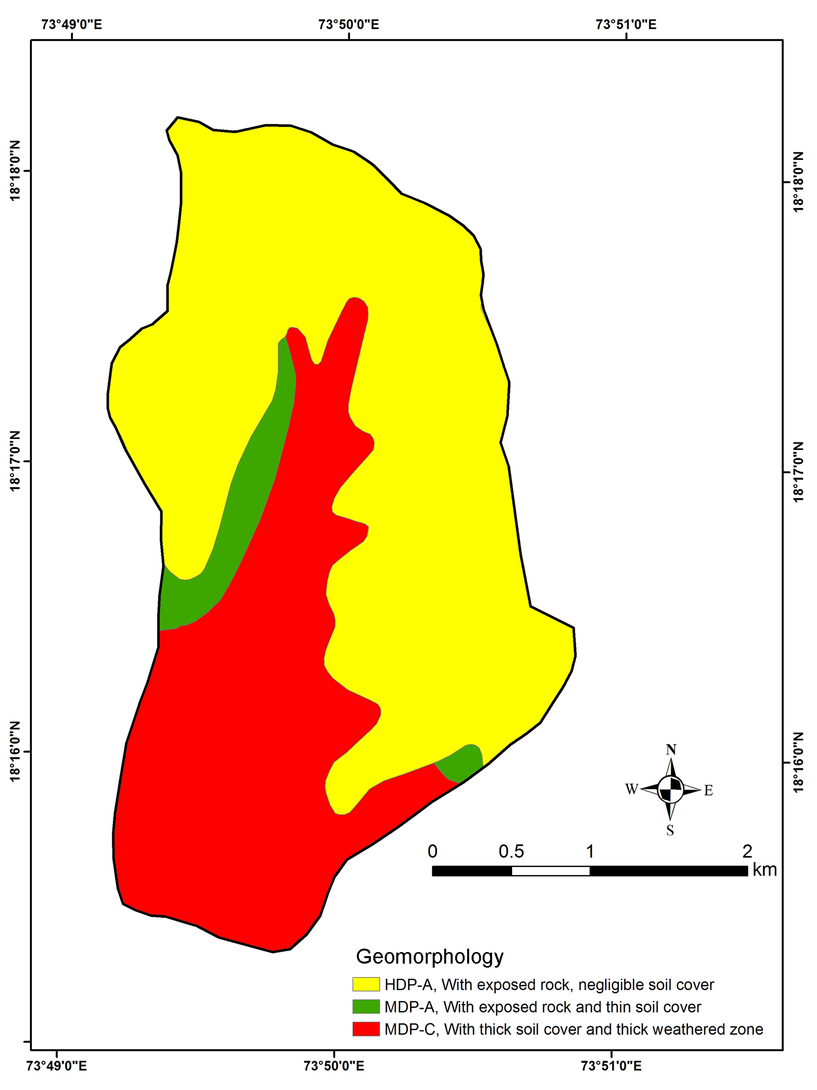
Schumm used the inverse of drainage density as a property termed constant of stream maintenance (Schumm, 1956). Constant of channel maintenance is the ratio between the area of a drainage basin and the total length of all the channels expressed in per sq.km. Constant of channel maintenance is dependent on the rock type, duration of erosion, relief, permeability, vegetation cover, and climatic condition. Schumm (1956) classified constant channel maintenance (km²/km) into five different category i.e. more erodible (<0.2), moderate erodible (0.2 to 0.3), moderately low erodible (0.3 to 0.4), low erodible (0.4 to 0.5) and least erodible (>0.5) (Schumm, 1956). The constant of channel maintenance of the study area is 0.30 km²/km, which indicates that Kolavadi sub-watershed is moderate erodible.

4.3 Morphometric Analysis - Relief Aspects

Relief or gradient aspects are quite essential parameters of drainage basin analysis as they depict the nature of ruggedness and surface configuration. Relief ratio, relative relief, and ruggedness number are some significant parameters of relief morphometry that is examined in the sequel (Table 4).

3.3.1 Basin Relief (H)

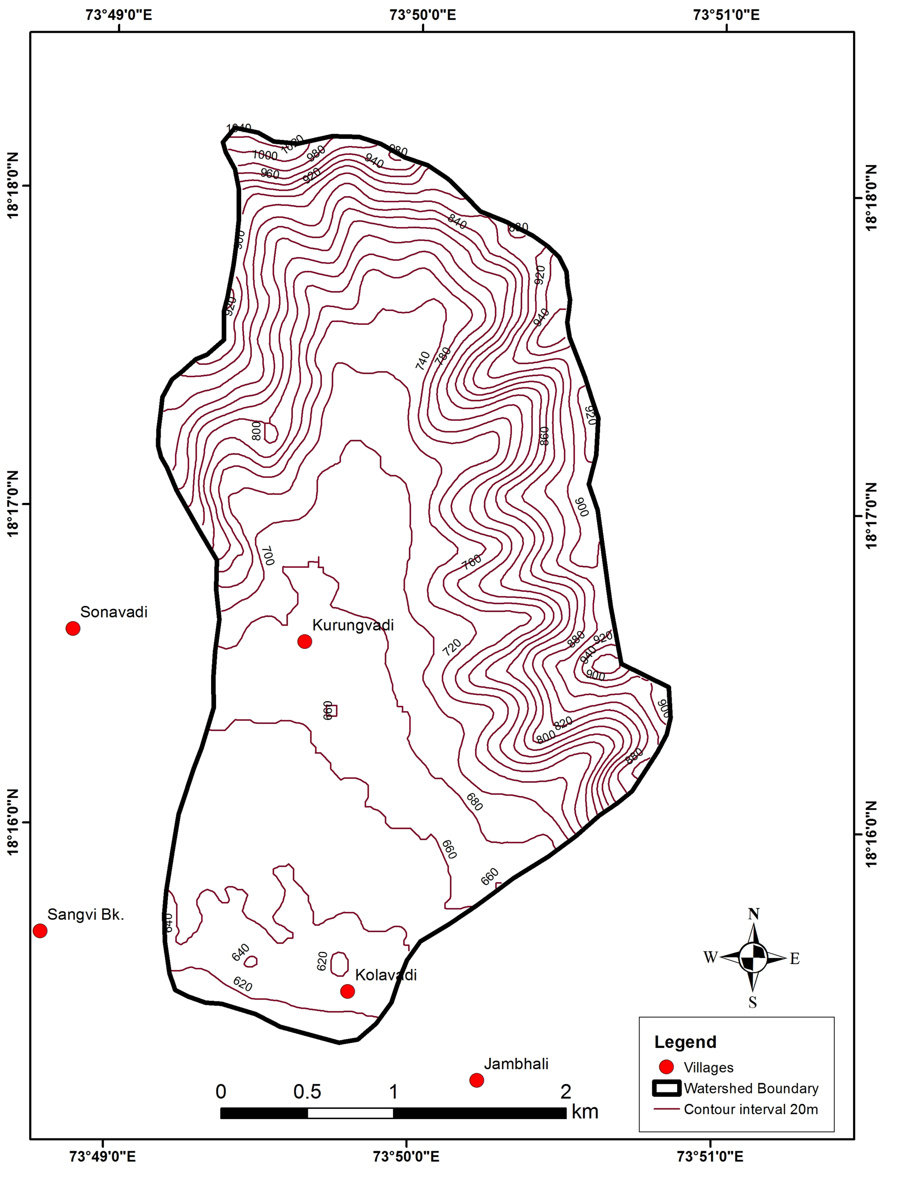
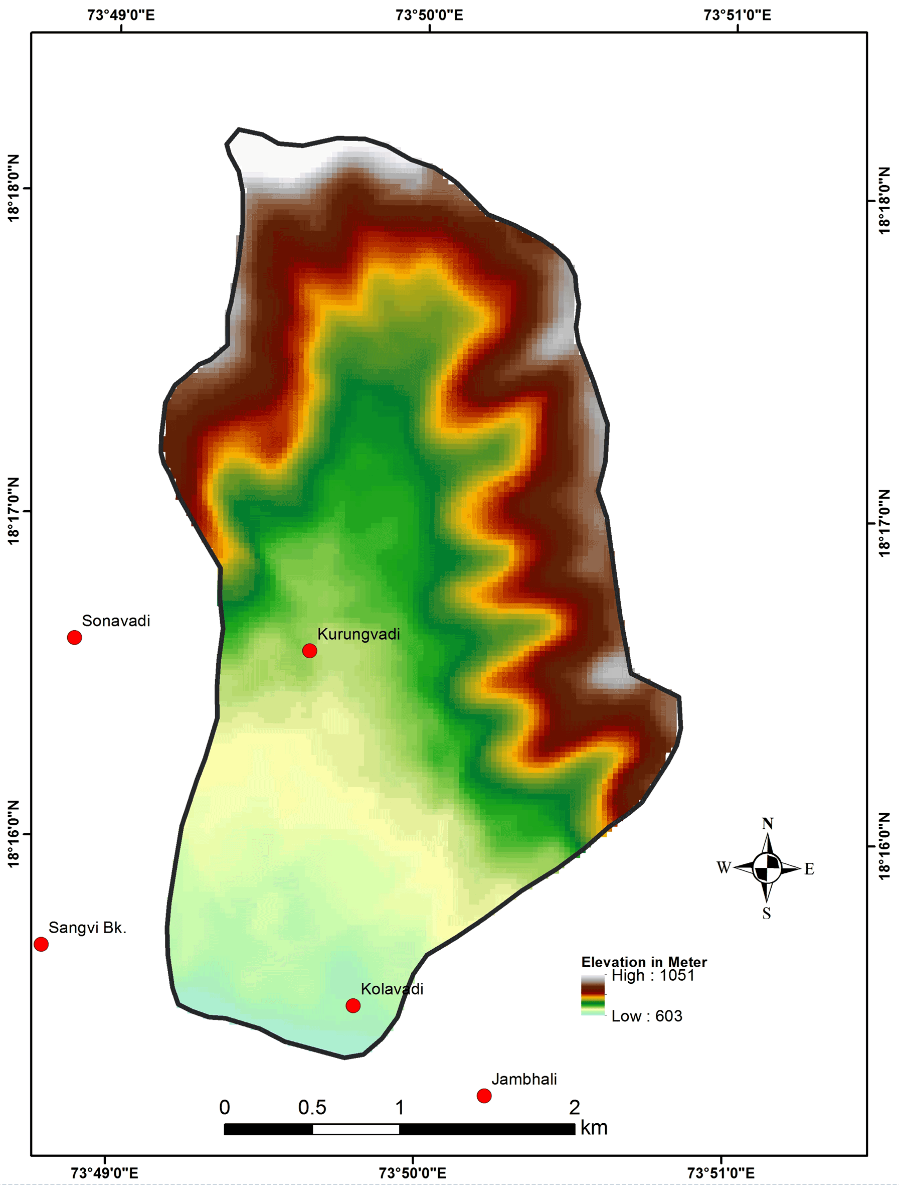
Strahler (1957) defined the complete relief of the river basin as the variation in the altitude amongst the highest position of a watershed and the lowest position on the valley floor. The Kolavadi sub-watershed average relief is 840m. The highest elevation of the watershed is a 1051m, and the lowest altitude of the watershed is 603m (Figure 6). The highest contour is of 1040m in the northwest direction of sub-watershed areas (Figure 5). The lowest contour is 620m in the southern part of the study area. However, the lowest elevation of the Kolavadi sub-watershed is 603m in the southern part.

Figure 5. Contours

3.3.2 Relief Ratio (Rhl)

The ratio between entire relief of a basin and the highest element of the basin parallel to the principal drainage channel is the relief ratio (Schumm, 1956). The one is representing the horizontal and the other passing through the highest point of the basin. It denotes the overall steepness of the drainage basin and the intensity of erosion process operating on the slope of that particular basin (Schumm, 1956). The value of relief ratio in Kolavadi sub-watershed is 0.07, which indicate low relief and moderate to gentle slope. The low value of relief ratios is mainly due to the resistant basement rocks of the basin and low degree of slope (Pareta and Pareta, 2011).

3.3.3 Relative Relief (RR)

Relative relief was a term introduced by Melton (1957).  A visual analysis of the study area was done with the help of digital elevation model (DEM). This DEM was produced based on contour data (Figure 6). The elevation varies from 603m to 1051m, which represent the land has gentle to a steep slope.

Figure 6. Digital Elevation Model

3.3.4 Ruggedness Number (Rn)

Ruggedness number is the output of maximum basin relief and drainage density, where both parameters are in the same unit (Strahler, 1950). In some times, both variables are significant, and the slope is steep as well as long, that time ruggedness number occurs in enormously high values. In the present study area value of ruggedness number is 1.27. It is high, which indicates that it is highly soil erosion-prone area.

In spite of the study area, morphometric parameters being favorable for infiltration, floods are seen to occur during heavy showers of the monsoon season, which are characteristically high intense though in short duration. The resultant floods are due to inefficiency of the surface storage facilities like reservoirs, tanks and others.

3.3.5 Slopes (m)

Slope analysis is an essential factor in geomorphic studies (Horton, 1940). The slope is defined as the height rate of change in value from each cell to its neighbors (Todhunter, 1888). Lithology and the climatomorphogenic processes control the slope elements in the area with varying resistance. An understanding of slope plays a vital role in planning of agriculture, settlement, deforestation, and disaster management.

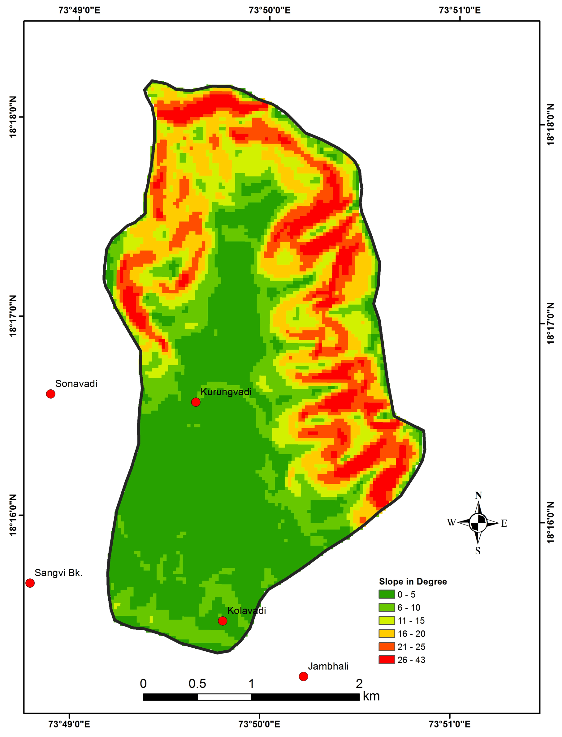
The lower slope values indicate flat terrain and the higher slope values show steeper terrain. The output slope dataset can be calculated as percent or degree of slope (Jensen, 2004). In the present study, the slope map is prepared based on the contours in Arc GIS platform. There are six classes of the slope identified and calculated in degrees. In Kolavadi sub-watershed area slopes vary from 0^o to 43^o. The southern and middle part of the Kolavadi sub-watershed is observed flat terrain and the northern part of the basin area which covered by a hilly area (Figure 7).

Figure 7. Slope

5 . CONCLUSIONS

The study of morphometric analysis with the help GIS technique can efficiently and precisely solve various watersheds related issues like droughts, soil erosion, watershed evaluation, flooding, groundwater potential analysis, etc. Many researchers have found that GIS-based approach in morphometric analysis of river basin is more reliable than the conventional methods. GIS technique is a simple, user-friendly, sustainable, and time-saving tool to study the sub-watershed areas with an output of good quality and a high degree of accuracy. It can be concluded that the morphometric variables of fourth-order basin of the area are influenced by lithology. The study has also brought out the varied characteristics of the drainage network about sub-watershed. The results, thus obtained, can be used in watershed management strategies. The values of the bifurcation ratio (2 to 4.5) indicate that the drainage basin is affected by structural disturbances. The high value of bifurcation ratio shows that mature topography with a higher degree of drainage integration. The sub-watershed basin has a less elongated in shape and a wide variety of climate and geology type. The computed values of drainage density and stream frequency highlight that the drainage basin is moderately drained. Relief ratio in the study area is 0.07, which indicate low relief and moderate to gentle slope. The value of ruggedness number is 1.27. It is high, which shows that it is highly prone to soil erosion.

All the outputs lead to the conclusion that the Kolavadi sub-watershed has the potential to perform its drainage function more effectively. Improving the storage capacity of the water bodies, rehabilitation and restoring channels to standard norms will enhance the sub-basins water holding capacity, which will be of immense use to meet the water demands of surrounding areas for agriculture and domestic purpose.

Tables

Figures

Conflict of Interest

Acknowledgements

Abbreviations

References