Abstract
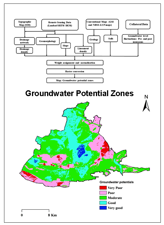
Present study is carried out for delineation of Groundwater Potential Zones (GWPZ) in Western part of Cuddapah basin, Southern India using Remote Sensing (RS), Geographical Information System (GIS) and Analytical Hierarchy Process (AHP). Various categorized thematic maps: geology, geomorphology (GM), slope, soils, lineament density (LD), drainage density (DD) and water levels fluctuations (WLF) were used for mapping and delineation of GWPZs. Suitable and normalized weights were assigned based on AHP to identify GWPZ. The GWPZ map was categorized into five GWPZs types: very poor, poor, moderate, good and very good. About 1.48% (6.05 km2) area is classified in ‘very good’, 25.95% (106.07 km2) in ‘good’, 47.11% (192.53 km2) in ‘moderate’, 22.12% (90.38 km2) in ‘poor’ and 3.34% (13.66 km2) in ‘very poor’ category. The acquired outcomes were validated with water levels fluctuations in pre- and post-monsoon seasons. GIS-based multi-criteria decision making approach is useful for preparation of precise and reliable data. The AHP approach, with the aptitudes of the geospatial data, various data bases can be combined to create conceptual model for identification and estimation of GWPZs.
1 . INTRODUCTION
Nowadays, around 34% of the world’s water resources are groundwater and a significant basis of drinking water is urban and rural areas. Andhra Pradesh is an arid and semi-arid region with actual flighty rain; so the average rainfall is less than a third of the global average rainfall (Zeinolabedinia and Esmaeily, 2015). Sustainable improvement of groundwater asset requires exact quantitative appraisal with the advent of powerful and high speed computers, the techniques for groundwater management of progressed, of which RS and GIS are of great importance (Chowdhury et al., 2009). Understanding of RS and GIS has demonstrated to be a powerful apparatus in the study of groundwater considerations (Krishnamurthy et al., 1996). GIS is defined as system for gathering, arranging, recovering, managing and showing spatial information into improved structure. In any case, contrasted with these strategies, remote detecting can be utilized as an efficient and savvy instrument for the synoptic study and analysis (Prasad et al., 2008; Deepika et al., 2013). As a device, remote sensing and GIS uses satellite representation for systematic study of height models, soil thickness, slant of the region, topography, geomorphology, precipitation, dissemination of groundwater, etc. The feasible improvement of groundwater asset requires exact quantitative appraisal. Profoundly escalated improvement of groundwater in specific zones of the nation has experienced over-use, prompting decrease in groundwater levels (Rajasekhar et al., 2018c, 2019).
In addition, GIS gives an outstanding methodology for resourcefully management of huge and compound spatial data for the management of groundwater (Machiwal et al., 2011; Rajasekhar et al., 2018c). AHP approach introduced by Saaty (1980) wherein a pair-wise comparison of various influencing parameters
is taken into consideration to calculate the final normalized weights of parameters (Agarwal et al., 2013). The multi-criteria decision analysis (MCDA) evaluates numerous differing criteria involved (Jha et al., 2010), which not only increases the precision of outcomes but also helps to decrease biasness on any influencing parameter. Recently, numerous studies have shown that the MCDA is less expensive and time saving technique for groundwater investigation and planning (Kadam et al., 2017). Appropriate development and sustainable management of the groundwater assets are fundamental since irrigation and domestic accomplishments can harm the spring and diminish the accessible natural resources (Mohamed and Elmahdy, 2017). The various studies on the application of geospatial tools with AHP and multi-criteria methods for identifying artificial potential zones have been carried out by limited researchers (Rahmati et al., 2015) Further, the combination of geospatial and MCDA approaches has been used in the study area.
In this study, an AHP approach with geospatial techniques for identifying GWPZs have been undertaken for the management of green growth groundwater resources in western part of Cuddapah, Southern India.
3 . METHODOLOGY
Present work is an attempt to fulfill the objective of identifying the GWPZs in Western parts of the Cuddapah basin, Southern India using various thematic layers such as geology, geomorphology (GM), slope, soils, lineament density (LD), drainage density (DD) and water levels fluctuations (WLF) are considered together through information based weighted overlay analysis (WOA) through AHP technique to prepare GWPZs map using methodology shown in Figure 2.
3.1 Preparation of Thematic Maps
Various thematic maps such as geology, geomorphology (GM), slope, soils, lineament density (LD), drainage density (DD) and water levels fluctuations (WLF) were prepared using ArcGIS software and ground truth data. The LULC layer was prepared using Landsat 8 satellite dataset with the help of image classification technique in ERDAS Imagine software (Rajasekhar et al., 2018a, 2018b). The drainage density map was prepared using topographical sheets from Survey of India (SOI). The soil map was prepared using district soil resource map by irrigation department, Cuddapah. The slope map was derived from the ASTER DEM data from NRSC Bhuvan website. The groundwater fluctuations of pre-post-monsoon data were collected from CM dash board, Government of Andhra Pradesh for various rain gauge stations for the period from 2018-19. The lineaments were digitized from satellite imagery using ArcGIS software (Chowdhury et al., 2010). An aggregate of eight thematic layers with their inter-relationship, which is inferred to incite the GWP in the western part of the Cuddapah district were chosen.
3.1.1 Geology
The study area composed of a stratigraphic sequence of rocks of Papaghni group and Chitravati group of lower Cuddapah Super group of rocks (Figure 3). Lithology of the study area has a series of alternate bands of argillaceous and arenaceous rocks. Igneous activity is seen between Vempalle formations and below the Tadipatri shale formation (Nagaraja Rao et al., 1987). Geology maps were prepared based on ground water and mineral resources map (GSI) and LANDSAT imageries by using ArcGIS 10.4 Software. Various types of rock formations and geographically based imagery based on tone, texture, and drainage patterns. This map shows various features like rock formations and their stratigraphic position. This map is organized based on lithology map of Andhra Pradesh on 1:50,000 scales prepared by the Geological Survey of India (Figure 3). According to the PCM of lithology layer was moderate response on the importance of aquifer formed in the groundwater. In the present study, geology was classified on the basis of aquifer response, the vempalli dolomite is major priority and shales have minor priority on the storage and infiltration of groundwater.
3.1.2 Geomorphology
Geomorphology of an area is a crucial element in evaluating the groundwater capability prospects due to the fact its faraway control of the subsurface motion of natural resources. The nature of the look at place is characterized by using dominantly with the aid of a few degrees hydrological backgrounds the geomorphology of any province is a crucial component in explaining the ground water capacity and is dependent on the lithography and shape of the basic formations (Kumar et al., 2016). The substances associated with the vempalli formation. The geomorphological function in the area may be categorized into 8 types i.e. river / water body, floodplain, pediment pediplain, structural valley, structural hills and ridges (Figure 4). The geomorphology of have a look at place is a dominance of porous sedimentary rock spatial quantity of the floor water bodies such as river become protecting 1.85% of the observe location, which act as recharge sector regarding the groundwater capability. Geomorphological response on aquifer in WOA analysis, the structural origin has lower priority and denudational origin having higher priority in the storage of groundwater in the aquifer.
3.1.3 Lineament density (LD)
Lineament concentration may be future to the volume of the consequences of tectonic alteration, rock splitting and shearing and groundwater prospects. Thus, the calculated linear density is a massive and useful method for the software of the maximum applicable facts in the subject of linear substances. Related to imprisonment inside, the concentration area is within the study region. Lineaments are often analyzed by way of frequency histograms (Hung et al., 2005), LD maps (Zakir et al., 1999). The maximum not unusual method is to analyze the relative density of regions in line with part extent (quantity / km²), or the total duration of areas consistent with unit area (km/km²) or joining completely. However, there are hand clues. The essential hand is the variety of lineaments consistent with unit location (N-range/km²), the second predominant index is the whole lengths of lineaments in step with unit location ( \(Σ = NI \ L × 1 km/km²\) ), the main index is the full wide variety of intersections of region consistent with unit place (NI-variety/km²). There are two changed indexes, the fraction of the intersections (NI) versus the variety of lineaments (N) and the relation of the connections (NI) against the total duration of lineaments (L), which might be frequently used for reading fracture regions. The past changed index, the standard length of lineaments ( \(L_N\) ) is normally used by using this guide, we can decrease the dimensions of the lineament and the whole period of lineament. The linear density indices are considered for a positive grid cell decision, which may be positive on the basis of geometric map and may be reclassified in the stages of values and offered as a density map (Figure 5). The higher LD regions results the good sites for management of groundwater in the study area.
3.1.4 Drainage density (DD)
The DD pattern of an area is resolute by the nature and gathering of the bedrock, class of vegetation, precipitation assimilation limit of soils, invasion, and slant inclination (Manap et al., 2013). A low-drainage-thickness region causes more penetration and diminished surface overflow. It implies that regions having low drainage thickness are appropriate for groundwater improvement (Magesh et al., 2013; Dinesh Kumar et al., 2007). The drainage preparation of the investigation territory is appeared in (Figure 6). The seepage design was extricated straight for warmly from ASTER DEM ( \(28 \times 28\) m). The surface drainage thickness is the quantity of the aggregate of lengths of streams to the size of territory of the framework viable (Mogaji et al., 2015; Adiat et al., 2012). The drainage thickness file was determined through the qualities determined for every matrix was plotted at the focal point of the lattice utilizing ArcGIS software. At that point, the directions of the focal point of every framework were utilized to set up the surface seepage thickness map by addition strategy. Based on the surface drainage density, the study area can be clustered into five categories: 0.0-0.06 (low), 0.06-0.11 (moderate), 0.11-5.15 (high), and 5.15-7.35 (very high) km/km2 (Figure 6). The very high drainage density is observed in the Southern part of the study region. The low and very low drainage densities cover mainstream region.
3.1.5 Slope
Slope is individual of the significant fields which can be clarified via horizontal arrangement of the contours. In the vector form strictly spaced outlines characterize sharper slopes and thin contours. In the raster elevation, the slope is measured by using the identity of the maximum price of alternate rate of each cellular to neighboring cells (Bhunia et al., 2012; Sar et al., 2015). The slope values are considered both in percent and in both raster and vector paperwork framework (Figure 7). The slope amounted from digitized contours and see heights have shown that elevation reductions from the Northern component to the Southern part with slope 0º to 10º in flat and hilly regions, respectively. The study area is categorised into five categories: namely, 0-5º, 5-20º, 20-30º, 30-40º, and >40º (Figure 7). In the close to (0-1º), the runoff is slowed down, in which the strong slope area (10-15º), facilitates excessive runoff allowing less time for rainwater then comparatively much a lesser amount of infiltration and groundwater recharge ability.
3.1.6 Soils
The soil of the area has originated from the sedimentary beds underlying the area. Clay soils are generally found associated with the sedimentary shale, and quartz porphyry and darker soils are associated with the basic and ultra-mafic rocks of the dolomite, shale, volcanic flow. The soil in the study area exposes five main soil groups, namely skeletal reddish brown, fine gravelly clay, gravelly clay deep dark, moderately deep dark brown and water body (Figure 8). Rank of soil has been given on the basis of their access rate. Skeletal deep reddish brown soil has high infiltration rate, hence given higher significance, while the clayey soil has least infiltration rate hence assigned low priority.
3.1.7 Groundwater level fluctuations (GWLF): pre- and post-monsoon seasons
Water ranges in aquifers replicate a dynamic balance among groundwater recharge, storage, and discharge. If recharging exceeds discharge, the volume of water will increase; if discharge exceeds recharge, the extent of water stages will fall. Because they may not be distributed uniformly in space and time, groundwater stages are constantly growing or falling to the ensuing imbalances. Water levels in wells replicate those modifications and offer the predominant method of following changes in groundwater levels. High water ranges arise inside the rainy season where as recharging from precipitation exceeds discharge; low water levels arise at some point of the dry summer while discharging through evaporation, evapotranspiration and seepage to streams (Zhao et al., 2018). The fundamental elements that infusion groundwater ranges are precipitation, movement stage, properly pumpage and inoculation. Pre- and post-monsoon water level maps were prepared in ArcGIS software as shown in Figure 9 and 10. There is variation in the water levels during the post and pre-monsoon period due to recharge and discharge of groundwater.
3.2 Criterions
An exhaustive technique for groundwater resource evaluation of particular area needs the thorough investigation of various thematic maps like Lithology, Geomorphology, Lineament density, Drainage density, Slope, Soils, and Rainfall so as to prepare the typical thematic maps were prepared from RS data, SOI maps and land maps associated to the collateral maps and field outline. The specifics of thematic layers prepared from RS information and field overview, composed with the groundwater potential outcomes (Rahmati et al., 2015; Mundalik et al., 2018; Rahman et al., 2012). The AHP weights are increased by the percentage of total weight to obtain the final weight. The average weight given to the geology varies from shale to dolomites for very low to very high potential of recharge, respectively (Table 1) (Kadam et al., 2017).
Table 1. AHP scale (Saaty 2008)
|
Scale
|
1
|
2
|
3
|
4
|
5
|
6
|
7
|
|
Importance
|
Equal
importance
|
Weak
|
Moderate
importance
|
Moderate
plus
|
Strong
importance
|
Strong
plus
|
Very strong
importance
|
3.3 Weights
AHP for determination creation in which the matter is isolated into different restrictions, dividing them in a various flattened structure, settling on choices on the near consequence of sets of components and making the outcomes (Saaty, 1999, 2004). Each topical layer has in excess of five classes, which shows the connections between these consistent classes are extremely intricate. Hence, for the connection between these nine thematic maps has been determined using AHP and connection between their different classes has been distinguished (Saaty, 1980). The procedure for loading the thematic maps and their relating classes is given in the figure 2.
In this study, AHP was used to estimate the weights of all relevant parameters that influence the potential of groundwater recharge in the study region. AHP implies an assessment of the significance between the parameters, the normalization and calculating consistency ratio (CR). Depending on the hierarchical order constructed, it is decided that the priority of the influencing factors recognizes the significance of the features at various levels of the hierarchy (Kaliraj et al., 2015). To obtain qualitative data, the factors that influence each level are compared in pairs. The Saaty scale from 1 to 9 (Table 1) is used to measure the relative importance of the factor (Saaty, 2008).
3.4 Pairwise Comparison Matrix (PCM)
A diagonal matrix was prepared by placing the values in the upper triangle and their reciprocal values are used to fill the triangular matrix. Expert’s judgment was used for PCM (Zolekar and Bhagat, 2015). In addition, the relative weights were normalized (Table 2). This fundamental eigenvalue is used to degree the consistency of ideas through an analysis of the consistency ratio (CR) (Saaty, 1980). A CR values lower than 0.1 can be considered as opinions with less uncertainty in weight determination (Kadam et al., 2019, Rajasekhar, 2019a, 2020). The Consistency Index (CI) is calculated using the equations (equation 1) and the comparison matrix (Table 2) to compare all parameters for calculating CR.
\(CI = { \lambda_{max} -n \over n-1}\) (1)
where, \( \lambda_{max}\) = average number of consistency vector and n = number of criterions.
The CR has been computed using the equation 2.
\(CR = { CI \over RCI}\) (2)
where, RCI = random consistency index, provided by Saaty (2008).
Table 2. Pair-wise comparison matrix
|
Criterions
|
Geology
|
GM
|
LULC
|
DD
|
LD
|
Pre-monsoon
|
Slopes
|
Post-monsoon
|
Normalized weight
|
|
Geology
|
1.00
|
0.50
|
0.50
|
4.00
|
4.00
|
0.50
|
1.00
|
0.20
|
0.11
|
|
GM
|
2.00
|
1.00
|
0.25
|
4.00
|
1.00
|
0.50
|
0.50
|
3.00
|
0.13
|
|
Soils
|
2.00
|
4.00
|
1.00
|
5.00
|
2.00
|
0.33
|
3.00
|
0.25
|
0.16
|
|
DD
|
0.20
|
0.25
|
0.20
|
1.00
|
0.33
|
0.25
|
0.20
|
0.33
|
0.03
|
|
LD
|
0.20
|
1.00
|
0.50
|
3.00
|
1.00
|
0.33
|
2.00
|
1.00
|
0.09
|
|
Pre-monsoon
|
2.00
|
0.50
|
3.00
|
4.00
|
3.00
|
1.00
|
3.00
|
2.00
|
0.20
|
|
Slope
|
1.00
|
2.00
|
0.33
|
5.00
|
0.50
|
0.33
|
1.00
|
0.20
|
0.08
|
|
Post-monsoon
|
5.00
|
0.33
|
4.00
|
3.00
|
1.00
|
0.50
|
5.00
|
1.00
|
0.20
|
Table 3. Criterions, sub-criterions and AHP weights for GWPZs
|
Criterions
|
AHP weights
|
Normalised weight
|
Sub-criterions
|
|
Geology
|
11
|
0.11
|
Dolomite
|
| |
|
|
Shale
|
| |
|
|
Quartzite / conglomerate
|
| |
|
|
Water body
|
|
Geomorphology
|
13
|
0.13
|
Anthropogenic terrain
|
| |
|
|
Denudational hill
|
| |
|
|
Structural hill
|
| |
|
|
Water body
|
|
Drainage density
|
3
|
0.3
|
0-0.6 km/km2
|
| |
|
|
0.6-0.11 km/km2
|
| |
|
|
0.11-1.7 km/km2
|
| |
|
|
1.7-2.3 km/km2
2.3-3.6 km/km2
|
|
Lineament density
|
9
|
0.9
|
0-0.03 km/km2
|
| |
|
|
0.03 - 0.09 km/km2
|
| |
|
|
0.09- 0.18 km/km2
|
| |
|
|
0.18-0.28 km/km2
0.28-0.47 km/km2
|
|
Soils
|
16
|
0.16
|
Clayey deep reddish brown soil
|
| |
|
|
Deep black Soil
|
| |
|
|
Fine gravelly reddish brown soil
|
| |
|
|
Clayey shallow dark brown soil,
|
| |
|
|
Clay deep dark reddish brown soil
|
| |
|
|
very dark brown silt soil
|
| |
|
|
Water body
|
|
Slope
|
8
|
0.8
|
0-5º
|
| |
|
|
5-20º
|
| |
|
|
20-30º
|
| |
|
|
30-40º
|
| |
|
|
>40º
|
|
WLF Pre-monsoon
|
20
|
0.20
|
0.00-1.87 m
|
| |
|
|
1.87-2.23 m
|
| |
|
|
2.23-2.64 m
|
| |
|
|
2.64-3.17 m
|
| |
|
|
3.17-5.42 m
|
|
WLF Post-monsoon
|
20
|
0.20
|
-1.83-0.80 m
|
| |
|
|
0.80-1.96 m
|
| |
|
|
1.96-2.78 m
|
| |
|
|
2.78-3.59 m
|
|
|
|
|
3.59-6.17 m
|
3.5 Validation
The accuracy assessment was carried out based on water levels fluctuations data for pre- and post-monsoon seasons from the study area. The results showed good accuracy along surrounding dug wells in the study area.
4 . RESULTS AND DISCUSSIONS
Groundwater is being more and more implemented inside the latest years due to improve in effective value for water. The symbols of groundwater presence are interrelated to rainfall distribution, geology, land use, slopes, topographic elevation, travelling strengths. In order to expect the groundwater capability zones, different the background of the character lithological varies by potentials. Integrated valuation of thematic layers using weighted guide intersection method, different based totally on GIS strategies having been determined to be appropriate for explaining groundwater potential zones explained by using various factors, for instance, lithology, geomorphology, slope, drainage density, lineament density, soil texture.
The GWPZs map (Figure 11) was prepared using overlaying all thematic layer and assigning the weights and rank in ArcGIS software. Common catchment zones for the both forms of potential show the significance of GWP. The CI for the various thematic maps are CI=0.1373 and CR=0.09 which is less than the threshold value of 0.1. It shows a high level of consistency.
The based on this criterion the analyses and the rank of assigned to sub-criterion, the final WOI was estimated to map the GWPZs in the study area. GWPZ area was categorized into four categories: poor, moderate, good and very good (Table 4).
The GWPZ results are indicated that 1.48% (6.05 km2) of the land is very good GWPZs having the agricultural land as land use type with loamy type of soil present on the gentle slope. While 47.11% (192.53 km2) area is moderately GWPZs, mainly the fallow land or land with scrub or barren land with sandy clay soil having moderate to low soil moisture and water holding capacity. This type of land can be easily converted into good land of irrigation by providing the water resources and increase the financial support by the local bodies.
The marginally suitable land is about 25.95% (106.07 km2) having good GWPZs with very less soil cover can be converted into the agriculture land by providing supplementary efforts as well as energies for rigorous irrigation managing procedures for farming. Only steep slopping area and water bodies are main area were agricultural is not possible having 3.34% (13.66 km2) land (Table 4). It also comprises groundwater assets that are precise significant for cultivation. The outcomes acquired were quantified and this procedure retained the accuracy assessment of the results was carried out by water levels fluctuations data of pre- and post-monsoon season in the study matched with good accuracy levels along surrounding dug wells in the study area.
Table 4. Groundwater potential zones
|
GWRP
|
Area
|
|
%
|
km2
|
|
Very Poor
|
3.34
|
13.66
|
|
Poor
|
22.12
|
90.38
|
|
Moderate
|
47.11
|
192.53
|
|
Good
|
25.95
|
106.07
|
|
Very Good
|
1.48
|
6.05
|


 ,
Raghu Babu K 1
,
Raghu Babu K 1
 ,
Pradeep Kumar Badapalli 2
,
Pradeep Kumar Badapalli 2