Keywords

Yemen , Red Sea , ETM+ , Landsat , Navigation , Bathymetry

1 . INTRODUCTION

Nowadays, the hydrographic survey used in ocean environment in many aspects. Red Sea with its famous coral reefs has an irregular bottom especially in coastal zone, thus the bathymetry is of vital significance for shipping safety. The conventional hydrographic surveying or measuring the water depth is accurate for point measurement (Li-Guang et al., 2005). Although typical methods of mapping bathymetry like ship-borne echo sounder (single or multi beam) provide accurate measures, but it unfortunately, need a lot of efforts and money especially for big areas (Hesselmans, 2000). Satellite images could use for mapping the areas as an alternative method. That method is capable for mapping the coastal waters bathymetry at any environments. The main disadvantage of using remote sensing for bathymetry measures is the mutable sea bottom effects on its readings (Pang et al., 2004). Thus, the using of remote sensing for mapping bathymetry considered as a very promising tool, as it yield a synoptic view over huge ranges at low cost (Hesselmans et al., 2000).

Optical remote sensing methods penetrate into the clear waters to up to fifteen to thirty meters. The electromagnitic waves penetrate sea water according to its wave length. The higher penetrating wave length is the blue (400nm), followed by red wavelengths (600nm). In addition to the wave length, there are also the optical properties of the water like organic matter and suspended sediments could affect the penetration (Stumpf et al., 2003; Mumby et al., 2004).

Many authors identified the uses of satellite data for measuring shallow water bathymetry, one of the satellite sensors used is Landsat Thematic Mapper (TM) sensor (Smith and Baker, 1981). Several remote sensing satellites have a specific sensor that can be used for water condition study such as ocean color, coral reef mapping, and sedimentation spreading extent. One kind of satellite that has a capability in water condition study is Land Satellite using optic sensor to detect various electromagnetic long waves that started from visible light wave, infrared (near and medium) and thermal waves (Hesselmans et al., 1997).

The satellite sensor depth estimation depends on the quantity of reflected light (that affected by many parameters like water clarity, depth diminution, bottom reflectance, suspended solids) (Baban, 1993). In comparison with field survey, the satellite images could use for mapping bathymetry more effective due to its global coverage, availability and low cost.

Many authors discussed the success using of different electromagnetic wave lengths in bathymetry studies (like Warne, 1972; Yi and Li, 1988; Kumar et al., 1997; and George, 1997). The optimum water conditions for achieving the bathymetry detection by satellite sensors were discussed (Polcyn and Lyzenga, 1979). Selection of optimum wave lengths used in bathymetry studies depends on the type of water environment, as the lake water different completely from estuary water or sea water.

Modeling of bathymetry was achieved by different authors using a specific regression analysis model (Stove, 1985, Ibrahim and Cracknell, 1990; Baban 1993; Diaz et al., 2019; Tripathi and Rao, 2002). Benveniste et al., (2019) and Wu et al., (2018) obtained the requirements for a Coastal Hazards Observing System. Many authors used Landsat sensors with its specific resolution data for studying reefs and shallow water environments and its changes (like, Luczkovich et al., 1993; Zainal et al., 1993; Holden and LeDrew, 1998; Andréfouët et al., 2001; Lubin et al., 2001; Hochberg et al., 2003; Yamano and Tamura, 2004; Ji, 2008).

Bathymetry based on passive optical remote sensing uses sunlight. This light penetrates into the water and maybe reflected by the bottom. As the light moves through water column, it is absorbed and scattered by substances in the water. We ascribe absorption and scattering to suspend and dissolved materials in the water; chlorophyllous material, and the colored organic material components. The bottom reflectance depends on the sediment (sand-mud) and whether vegetation is present. If the path length of the light through the water increases, more light is absorbed. Therefore, bright areas indicate shallow water zones, whereas dark areas show deeper water. We have proposed several methodologies in the past to translate optical image data to bottom topography. Lyzenga (1978) derived an exponential relation between the height of the water column and the measured irradiance levels (Hesselmans et al., 1997).

The principal goal of this work concerned to establish a new tool to reduce both efforts and money spent in producing bathymetry maps by traditional methods. That not mean we will exclude the traditional methods, but it will reduce trip’s numbers needed to cover the coastal zones.

2 . RESOURCES AND APPROACHES

In this section different resources and approaches used to achieve objectives will discussed in details.

2.1 Study Area

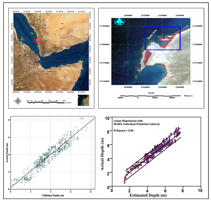
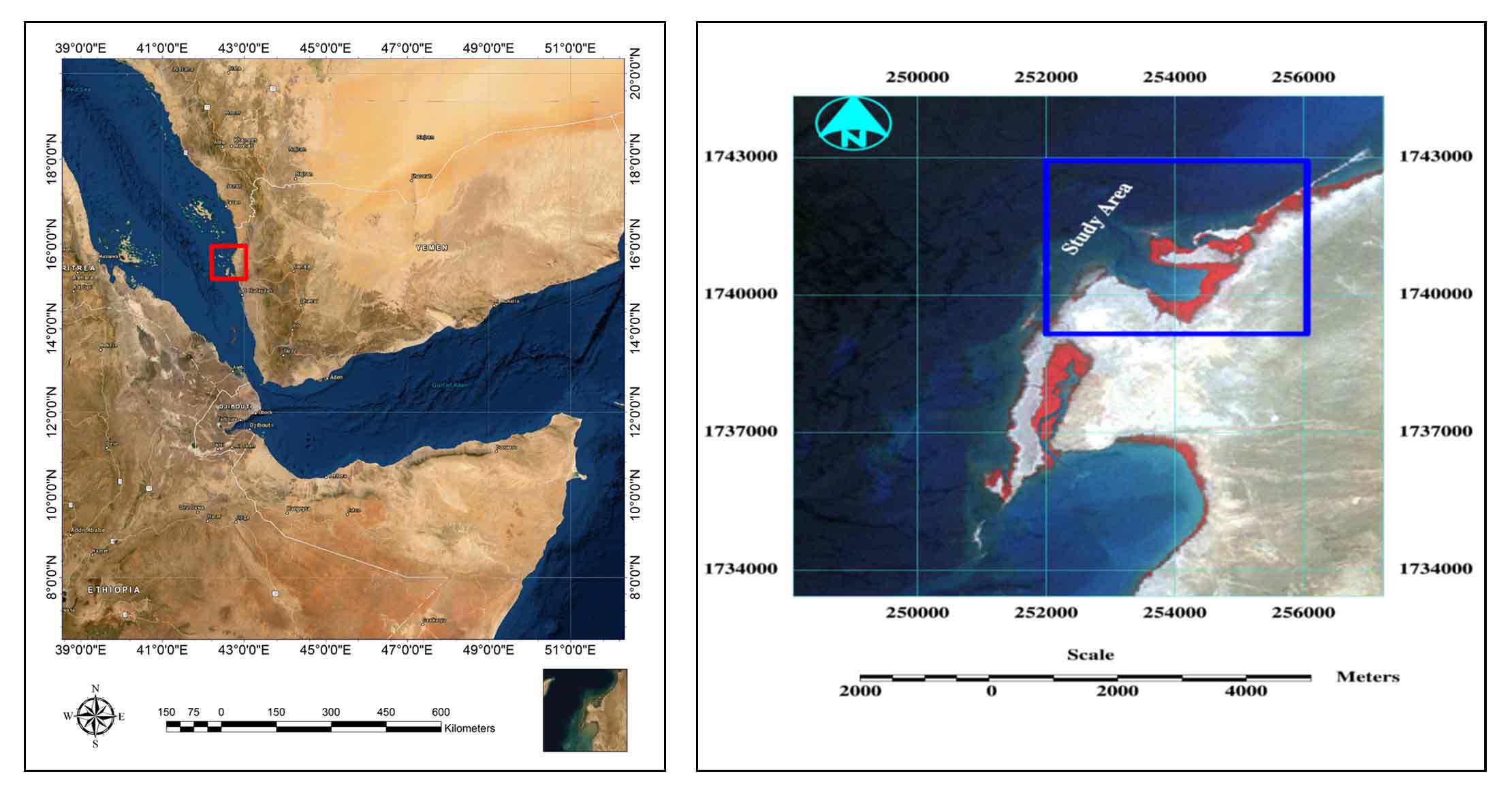
Al-Luhaia City is about 137 km north of Al-Hodeida and 20 km east of Antofash Island. The area of study location is north of Al-Luhaia town and is used by fishermen as a yard for their boats, it characterized by its important geographical position and by the bottom topography, and it covers an area 4.5 km (E) by 4.2 km (N). The approximate site center coordinates are 15°44ʹ 12.94887" N and 42°41' 33.36366" E (Figure 1). The availability of images by their geographical location and partly by the bottom topography partly governed the choice of this area.

Figure 1. Study area [Color Composite Images]

2.2 Field Measures

All marine field survey was achieved by the ‘Egyptian Hydrographic Company (Ehco) and Zone Engineering and Survey’ carried out for an approximate area of 5.0 km x 4.0 km in May 2003 using a Differential GPS (DGPS) system.

High accuracy range (±5 cm) was used the reason of using such accuracy is that to get precise position for depth measurements moreover for mapping accurate coastline. We used bathymetric measurements the Echo-Sounder device type NaviSound 205 and the Software which was used is Trimble (HydroPro). We have collected more than 4000 observations from the study area during one long working day under suitable weather conditions (average Temperature 27 ºC); these reading data comprise digital easting/northing/depth triplets as recorded by the navigation system DGPS and sounding equipment on a vessel. Soundings in the area used range from less than one meter down to a little over 9 m and are fairly well distributed throughout the range. The data then tested and filtered from unessential reading, the useful data then used for analyzing. Survey and field measurements have been done for Al-Luhaia Site and carried out for an approximate area of 5.0 km x 4.0 km. The sound measures were corrected to mean sea level (MSL). Depth value measured at any point was added to the tide value at that specific date and time (0.11 m).

2.3 Landsat ETM+ imagery

The images for the Al-Luhaia, main study area comprises path 167 row 49 in the Landsat Worldwide Reference System (WRS) (Figure 1). The image-base underlying this paper comprised Landsat-7 (ETM+) 8-Bit multispectral satellite imagery (06-02-2003) with nine different bands. The sensor pixel size is 28.5 meters for used spectral bands. The thermal infrared has a pixel size 60 m, it used to map the coast and line and merged islands also it can be useful for studying the surface features, whereas the visible bands provide the best water penetration. The ETM+ image characteristic for the Al-Luhaia study area can be explained in table 1.

3 . DATA PROCESSING

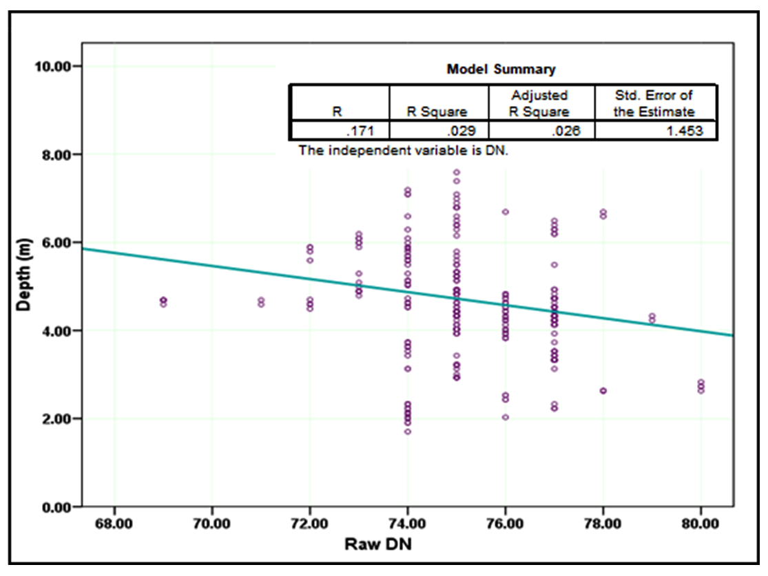
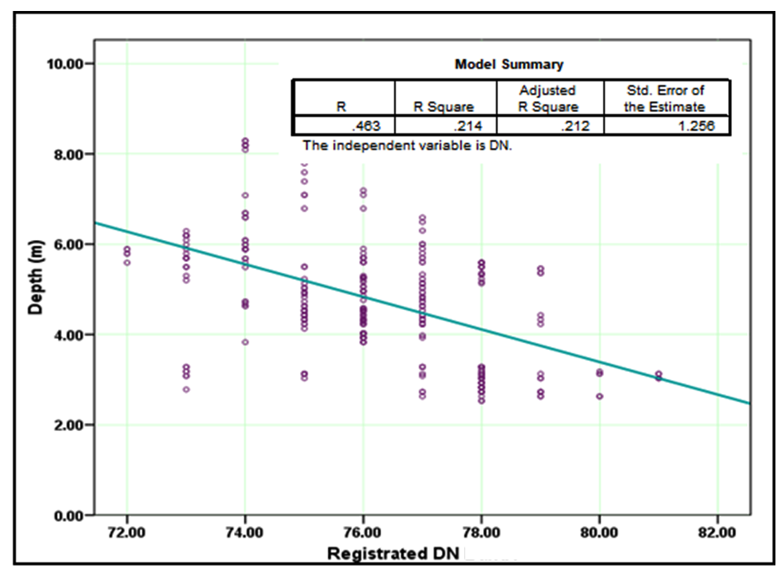
Data processing and analysis moves through several steps. First, the image ordered from the United States Geological Survey (USGS) was geo-referenced but not satisfied to achieve the bathymetry depths that correlate to the DN values. As illustrated in figure 2, it’s clear that the regression and correlation values (R² = 0.029 & R = 0.171%) revealed a very weak relationship between values of image digital numbers (DNs and water depth values measured directly through field survey, whilst after the re-registration for the same image band 1, a not bad improvement for regression and correlation relationship (R² = 0.214 and R = 0.463) revealed between DNs and water depth measurements as shown in figure 3, therefore it should re-register the images with the field water depth measurements.

Figure 2. Raw DN of band1 before rectification

Figure 3. Raw DN of band1 after rectification

As result of two different registration procedures 1^st and 2^nd polynomial orders that were used and show that the regression values (R²) were higher for the bands in 1^st polynomial order registration than 2^nd order, therefore the all analysis were carried out by using 1^st polynomial registration image. Table 2 shows the regression and correlation coefficients for the two methods that were used.

Second, as the image original digital number values have variances could affect the obtained result. The used image pixels values were averaging using low-pass filter to remove any anomalies. Several tests of low-pass ( \(3 \times 3, 5 \times 5, 7 \times 7 \ and \ 9 \times 9 \) ) filtering, or averaging of DN values, were applied. Table 3 shows the best filter, low-pass used for all bands and the regression and correlation values. The filter of size \(5 \times 5\)  represents the optimum filter window size. Blue, Green, and Red bands show the best fit, respectively. This shows that relationship is rather strong and was found to agree well (regression and correlation coefficients of 0.876 and 0.936).

We converted digital numbers to units of calibrated reflectance to calibrate images to surface reflectance. The overall accuracy for image shows improvement after the application of the DN converting to reflectance. Table 3 shows increasing in results between relationships of overall reflectance bands in the visible range with field depth that shows a model can estimate depths. A comparison of these results shows higher values in regression and correlation coefficients than the results that were obtained from low-pass filter \(5 \times 5\)   process, for example reflectance band 1 shows the regression results (0.944) while band 1 low-pass filter \(5 \times 5\)  gives (0.876). So we conclude that we should convert images to reflectance before any kind of analysis is taking place.

4 . REGRESSION ANALYSIS

We can achieve all algorithms for retrieval of seawater depth from Remote Sensing Reflectance into the empirical algorithm. It bases the empirical algorithms on the correlation between band reflectance ratios and water depth. This algorithm works well in Case I waters but is not reliable for Case II waters (Hommer and Carter, 2002).

Since the actual depth values collected, a simple linear regression used to compare measured water depths from field to pixel reflectance values in different spectral bands. Note that data were collected from clear water. We can express the simple linear regression model in the following form:

\(D_i = \beta_0 + \beta_1R_i\)                (1)

where,

\(D_i\)  is the value of the field measured depth in the i^th observation (dependent).

\(R_i\)  is the reflectance value in the i^th observation (independent).

\(\beta_0\)  is the R intercept of the regression line.

\(\beta_1\)  is the slope, and

                i=1… n  (n represents the number of observations).

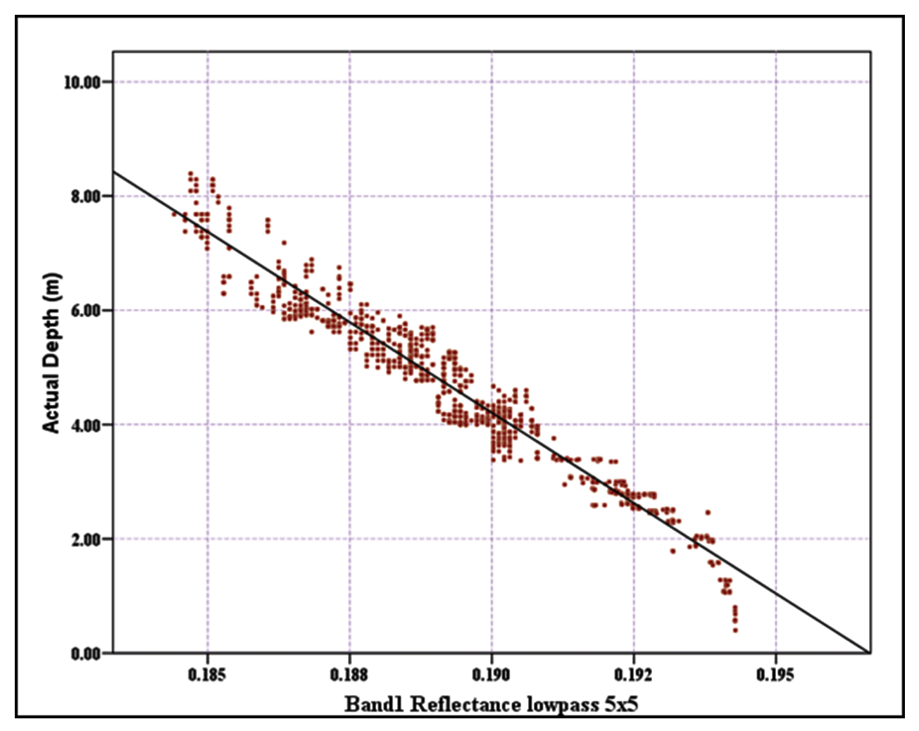
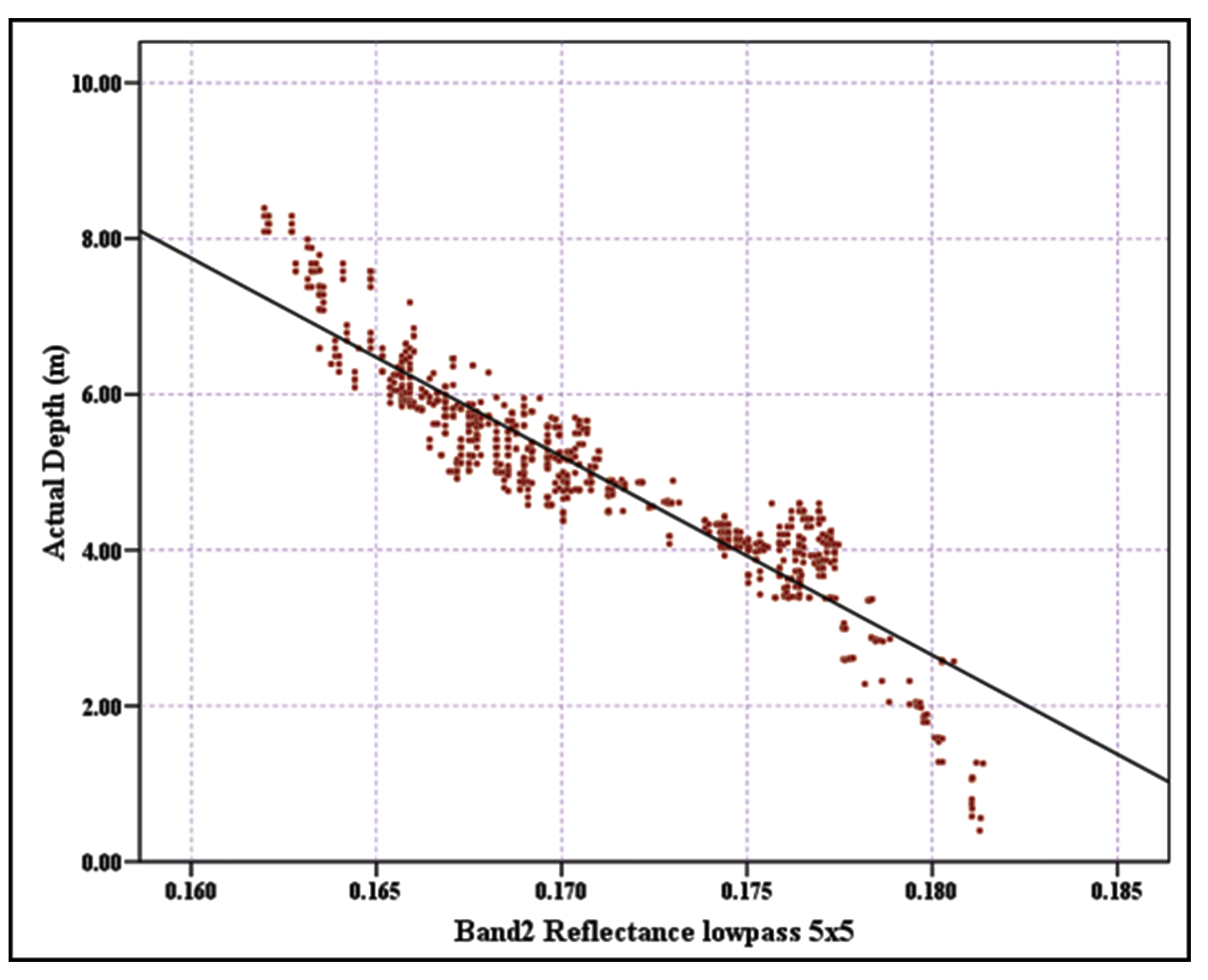
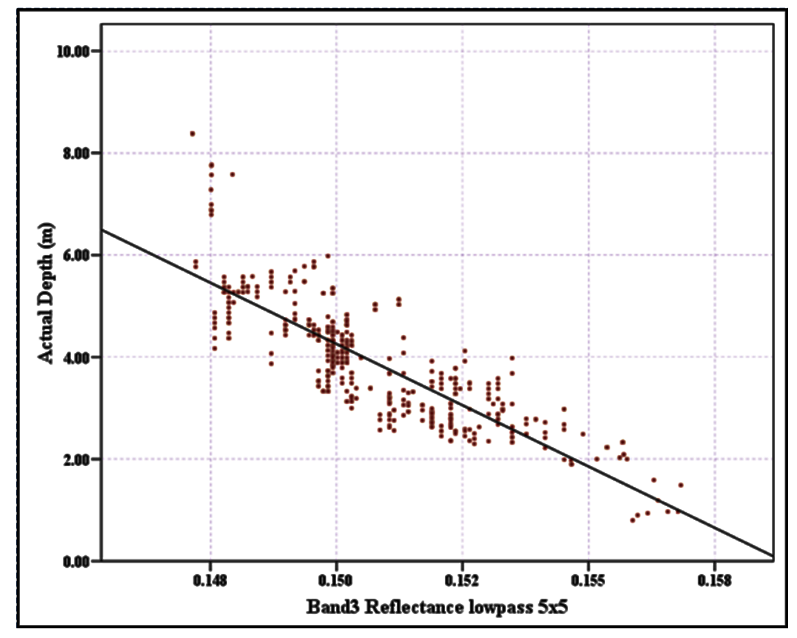
By using SPSS v.15 software, we could derive the estimated model, by estimating the coefficients of model (1) regression coefficients using the data. We plotted scattergrams of reflectance values against depth to select the fitting band for modeling depth (Figures 4, 5 and 6).

Figure 4. Regression model: Band 1

Figure 5. Regression model: Band 2

Figure 6. Regression model: Band 3

We carried the regression analyzes out to test a simple regression relationship between depth and reflectance (bands 1, 2 and 3). We compared the depths derived from a model to the ground truth observations for depths up to 9 m. It was noted, however, that a depth offset of 0.3 m was present between the data sets. The soundings, in the area used, range from less than one meter down to a little over 9 m and are fairly well distributed throughout the range. The total numbers of depth observations taken from this area were 1500 points.

Using the relationship between depth measurements and reflectance for visible bands, we created a model with the slope and intercept of the regression. We found this model that there is a general decrease in bands’ reflectance values with an increase in sea depths. We show the results for the regression analysis in table 4 and the resultant model equation created from Band 1 reflectance and actual depth was: \(\hat{D}=-633.08 \times R+124.49\) , the resultant model created from Band 2 data was: \(\hat{D}=-254.81 \times R+48.52\) , also for band 3 was \(\hat{D}=-480.21 \times R+76.29\) . The models were more accurate and fit well with an R² of 0.944 for the band 1, an R² of 0.863 for the band 2 and an R² of 0.692 for the band 3. The coefficients of regression and correlation between the band (one) reflectance and the actual measures represent the highest value. Thus, band 1, offering the highest coefficient of correlation, regression, and it represent the best band used in modeling the water bathymetry.  The clear water model for this cause was more accurate with correlation coefficient of 0.971 for depths up to 9 m. We applied results from the regression for band 1 to the Landsat-7 (ETM+) reflectance image, producing an estimated depth image by using ERDAS Spatial Modeler. We present the estimated depths prediction in table 5. The achievement of regression equations is for the structure of condition for the examining area into the configuration of this algorithm. However, some note that there is significant observable relationship between the reflectance (band 1) and field depths data. The correlation has significance at the 0.05 level and the p-value in the analysis of variance shows that the relationship is significant as well. Results from that model showed the potential for this band to be used to extract depth.

5 . VALIDITY OF THE MODEL

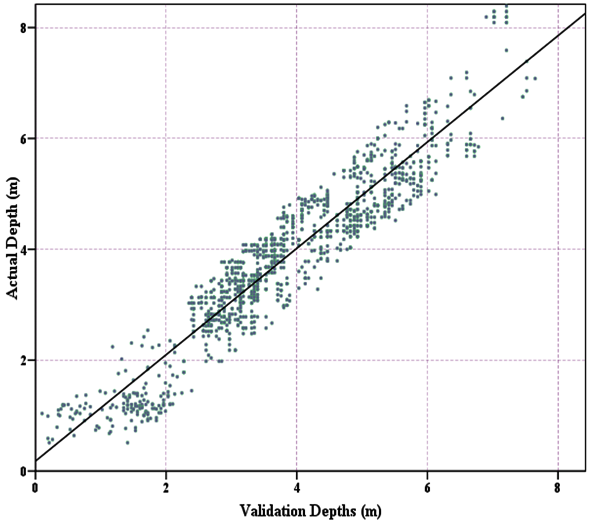
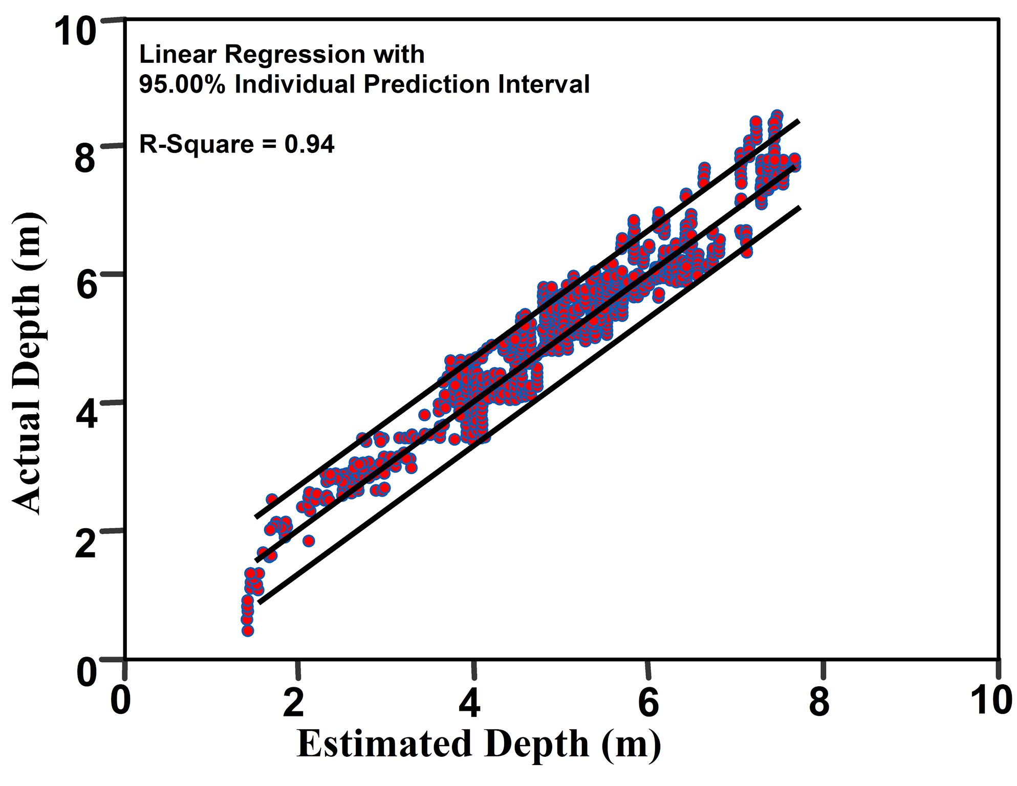
The regression analyses offered by the model have been verified using data from 1500 new depths locations.  Validation results show that a p-value was found significant relationship for the validation test at 95% confidence interval and 0.05, significance level. This validation test model also offered a very good correlation coefficient, 0.9385. As direct scatterplots between actual depths and the independent validation depth by model band 1 are shown in figure 7, give a pure outcome (R²=0.916). Accordingly, validation model was accepted and ready for used in bathymetry estimation.

Figure 7. Al-Luhaia regression model for band 1 versus unused actual depth

6 . ACCURACY ASSESSMENT

We have calculated the accuracy assessment using the in situ depth data (1500 points) and the estimated depth from the actual depth and pixel reflectance by the regression model algorithm after Louchard et al., (2003): 

\(Estimated \ Error = {Estimated \ Depth - Actual \ Depth \over Actual \ Depth} \times 100\)        (2)

Both clarity and depth of water affect accuracy. The accuracy of depth values estimated in clear water was 95.92%, while the coefficient of correlation was 0.97 (estimated error = 4.08%). Depth values ranged from less than 1 up to 9 meters. However, when the depth goes over 8 meters, the standard error increases because of the absorption of the electromagnetic wave through the water. Although the models created and the methodologies of field measurements were accurate, still there was minor errors in-depth accuracy as mentioned above (4.08%). These errors need to be overcome since navigation requires high accuracy. To do this a safe factor which should be more than the maximum error recorded must be added or subtracted from depth estimated by the bathymetry models. This will give us a safe range within which the will fall the correct depth.

7 . NAVIGATIONAL SAFE FACTOR (PREDICTION INTERVAL)

Since we have the estimated depth based on actual depth and pixel reflectance, then it is essential to extract a new safety depth using safe factor e. To find the prediction interval, equation (equation 3) has been employed.

\(\hat{D}_{new}=\pm t_{(\alpha / 2; n-2)} \times S\{\hat{D}_{new}\} \)         (3)

where,

\(\hat{D}_{new}\)  is the new depth to be predicted.

\(\alpha\)  is the confidence level.

\(S\{\hat{D}_{new}\}\)  is the standard deviation of \(\hat{D}\)  and given by the following formula:

\(S^2\{\hat{D}_{new}\}=MSE \begin{bmatrix} \frac{5}{6} + {(R_d-\bar{R})^2 \over \sum^n_{i-1} (R_i-\bar{R})^2} \end{bmatrix}\)

MSE is the mean square error, \(R_d\)  is the desired reflectance point e.g. (R = 102), \(\bar{R}\)  is the average reflectance which equal (0.183).

 Example 1: Consider a navigator has estimated depths for certain area and needs to navigate with more safety and security depth under the ship draft. If they wish to predict the new depth at an estimated depth point of 8 m with 95% as confidence level, then apply equation (3) with MSE = 0.350 (See table 4) to get a prediction interval.

\(7.230 \leq 8 \leq 8.770\)

With a confidence prediction of 0.95, the navigator predicts that the maximum depth would not exceed 8.770 meters and the minimum would not go down 7.230 meters. The safe factor would be \(\pm 0.77\)  meters. As a navigator responsible for the safety of the crew and the ship it should take the minimum predicted value into consideration. Another approach if the navigator has a list of estimated depths, such as the depths shown on Figure 8, would be to take the maximum error to apply the safety factor, so if he takes the ED of 9.5 m the interval will be:

\(8.730\leq 9.5 \leq 10.270\)

So the safe depth for navigator will be 8.730 meters.

Figure 8. Predicted interval of Band 1 for Al-Luhaia area (clear water)

8 . DISCUSSION

The mean of bathymetry measures in this work are the usage of low-cost Landsat-7 (ETM+); GPS (locating sampling points); optimum spectral band; accurate least-squares regression link between depth and reflectance value. Blue band (band 1) reflectance was used to feed the regression model. Although Al-Luhaia port was selected as a case study in this paper, some important facts related to band selection, use of GPS and linear regression model approach have emerged, which may apply to many coastal and port areas. Remote sensing has offered very useful bathymetric maps of the Al-Luhaia area and similar maps can be generated for other coastal regions.

The differences in the regression model revealed that the model results were not valid for depths greater than 8 meter for the blue band because of the light diffuse as the depth increase which causes the absorption of light energy which does not encourage result and not support the research aims for updating nautical charts. International Hydrographic Organization (IHO) has set up the accuracy requirements for soundings as 0.3 m for depths up to 30 m, 1 m for depths from thirty to hundred meters, and one percent of the depth, for water depths over 100 m (Baban, 1993). Therefore, this study presented encouraging result which could help in deriving bathymetry maps of shallow coastal areas less than 7.5 m.

Tables

Figures

Conflict of Interest

Acknowledgements

Abbreviations

References