Keywords

Decision making , DEPEND , INTENT , Modeling , Motor Vehicle , Structural Equation Modeling , Transportation , Urban

1 . INTRODUCTION

Automobile dependency refers to a medium of transportation depending on land use pattern which favors automobile access and provides inferior alternatives such as cars, vans, light-trucks, motor bikes and so on. In this century, surface transport has become more increasingly automobile dependent. Recent research shows that increasing of private motor vehicle travels is necessarily good for economy or society. Besides, beyond a certain level it may impose more loss than benefit. Some of the benefits are direct but a lot of costs are indirect and cumulative that are not bear directly by users (Litman, 2016). A study from World Bank shows that automobile dependency reduces regional imbalance in economic development (Kenworthy et al., 1997).

Meanwhile, private motor vehicle dependency is higher in outer and peripheral area of the city than the residential areas (Dupuy, 1999; Newman and Kenworthy, 1989) which leads to lower density and urban sprawl development. In this circumstance, this phenomena increases economic, social and environmental cost (Burchell et al., 1998; Kharizsa et al., 2015). Dependency of private motor vehicle has many impacts on human lifestyle and national economy. It increases mobility and convenience to motorists and all together it increases traffic congestion, roadway risk and environmental impacts also (Raad, 1998; Litman, 2016; Song and Wang, 2017). The car sharing is continuously increasing in the urban area and therefore, the city is characterized as car dependent (Dupuy, 1999; Newman and Kenworthy, 1989). This reliance influences show high level of car ownership (Collet, et al., 2013; Ochieng and Jama, 2015). A report called Dhaka Tribune shows that, in Dhaka, around 6-8% of commuter use cars that takes 76% of occupancy in roads. Meanwhile, other transport uses 7% that helps to create congestion. World Bank study exposed that every day the people of Dhaka is losing nearly 3.2 million working hours owed to traffic jam and the loss amount is about Tk. 30000 corer (Rimon, 2017).

As the developing country, Bangladesh has several problems where traffic congestion is one of them. It is composed of several factors and issues among them own motor vehicle use is more significant. Maximum are depending on it due to less travel cost, time saving and comfort. On the contrary, it helps to create sever congestion on road that take charge of time consumption. Again, it also worth of loss number of working hours and money that is reported by Bangla Tribune in 2017. Having individual satisfaction and benefit private motor vehicle dependence also creates dissatisfaction in social life like congestion, pollution, mental illness, behavioral changes and so on (Litman, 2001). Therefore, it is important to find out which indicators are more influencing for its dependency and hence take steps to available those facilities to people that will help to reduce the dependency.

Structural Equation Modeling (SEM) is a sound and efficient way to measure inter complex relationship with various influencing factors. Influencing factors related to transport and related hypothesis with the factors can be evaluated using SEM method (Zhao, 2011). This study intended to measure dependency of private motor vehicle and its influencing factors with their influencing rates. In order to measure private motor vehicle dependency and its factors, this research uses the Structure Equation Method (SEM) also to identify reasons behind the behavioral approach. This is important because transportation is itself a major economic sector and it causes to all other sector virtually.    

First aim of this study is to investigate the influencing factors for private motorized vehicle dependency and its preferences and second one is to estimate Structural Equation Model (SEM) for quantifying subjective motor vehicle dependence and to examine its determinants. The factors like social status, monthly income, family size, cost of private and public transport, etc. influence use and dependency on private vehicles were assessed. This paper also analyzed people’s preferences to private vehicles.

2 . METHODOLOGY

The survey was conducted for 130 randomly selected persons to collect the information lifestyle and dependency on private motor vehicles in the year of 2018. This study uses SEM for quantifying subjective motor vehicle dependence. It is a multivariate statistical analysis approach that is used to evaluate the relationships. This approach is a mixture of factor analysis and multiple regression analysis that is used to evaluate structural relationship between observable variables and latent constructs. Experts prefer this approach, as it measures the multiple and interrelated dependency in a single study. For this analysis two types of dependent and independent variables were used. SEM is a mathematical approach for the creation and testing of statistical models, also known as casual modeling while evaluating the proposed casual relationships. As SEM is a way of finding the weighted value of each variables that shows a cause-effect relationship between dependent and independent variables (Hox and Bechger, 1998), so this method is used here to show how the indicators are related and how they are influenced with each other. It is also used for finding the weighted value of each dependency factors. All the factors are placed under three latent variables that is MOTOR VEHICLE USE (MVU), DEPEND and INTENT. The statements under those three latent variables are assigned in five response level, e.g. strongly agree, slightly agree, neither agree nor disagree, slightly disagree, and strongly disagree, which are inputs as 2, 1, 0, -1 and -2, respectively. Individual dependency on private motor vehicle is measured as latent variable ‘DEPEND’ and intention to reduce private motor vehicle use is measured as latent variable ‘INTENT’ shown in Table 15.

To quantify individual private motor vehicle dependence, three indictors have been used: i1-deals with an entire assessment; i2- reviews from the perspective of choosing their travel modes; and i3- inquiries about the mentality of changing for alternative options. At the same time to quantify people’s intention to reduce private motor vehicle use two indicators: i4 (I am eagerly trying to use my motor vehicle less) and i5 (I am not willing to reduce my motor vehicle use) were used.

To explore the relationship among demographic, socio-economic condition, a simple average value of the indicators was used as the initial values for DEPEND and INTENT. Again, density of living place, having children and income is considered as indicator of actual private motor vehicle use denoted as motor vehicle use (MVU). All those data are processed by MS Excel, IBM SPSS, and AMOS software after collecting and analyzing all the primary and secondary data.

3 . RESULTS AND DISCUSSIONS

3.1 Descriptive Statistics

At the beginning of the study it was assumed that, income, social status, surrounding of users influence more to use the private motor vehicles. As the greater the income, the greater the social status is, hence it plays a vital role for using own vehicle. It is an indicator of social prestige. Again, if having children, it influences more to use own vehicle for safety and it increases the trip purpose and frequencies.

Surveyed data can be concluded that some variables have large or moderate significance in private motor vehicles. Population density of the areas, having children, income, initial cost, fuel cost, repair cost, average speed of the vehicles and social status or grade are one of the influencing factors behind private motor vehicle using.

About 41.54% PMV users are observed in highly dense areas, 49.23% in moderately dense areas and 9.23% in low dense areas (Table 1). The rate of motor vehicle use is moderately influenced by population density (Table 1). As Bangladesh is a developing country, most of the people are middle class society tend to live in middle or highly dense areas. As most of the respondents are belonging to middle class generally prefer motor bikes (Table 2). PMV users from low income category (<15,000 Tk.) are 16.15%, middle income category (15,000-30,000 Tk.) are 44.62%, moderately high income category (30,000-50,000) are 22.31% and high income category (>50,000) are 16.92%. The middle income people tend to dependent on PMV. People from low income group are relatively less dependent on private motor vehicles. The income has large influence on private motor vehicle uses. Availability of public transport is shown in the table 4.

About 76.92 % population is depending on private motor vehicle. Car users are 20% and other users like own private taxi or auto are 3.08%.

Respondents are classified into A, B, C and D social grade based on their income and expenditure ranges (Table 5). PMV users from grade ‘A’ are 17%, ‘B’ are 22%, ‘C’ are 41% and ‘D’ are 16%. Respondents from low income classes tend to relatively low dependent on private motor vehicles.

In general, people from higher income groups prefer comfort and less time for their journey. In our society, having private motor vehicles is a symbol of better status. People from middle income groups prefer to have private motor vehicles like motor bikes to avoid travelling hassle. Relatively well-off families do not have any intention to reduce their use of cars. As in our country, transport authority cannot be able to provide sufficient and comfortable public transport facilities, people cannot be able to concern about environment to reduce their use.

MVU having children are 65% (Table 6). People from the age group, 30-40 years are depending on PMV for education purposes and have private motor vehicles. Now-a-days people frequently use their vehicles to send children to school, tutors, etc. Having children is positively co-related with the rate of motor vehicle uses, it is negatively co-related with the intention to reduce motor vehicle uses. About 5% people use private motor vehicles for only for education purpose (Table 7), 10% people use for work and education purposes, 5% people use for education and recreation purposes, 4% people use for work, education, recreation purposes, 4% people use for work, education, shopping purposes, 3% people use for work, education, others purposes, 8% people use for education, shopping and recreation purposes, 6% people use work, education, shopping, and recreation purposes, 8% people use for work, education, shopping, recreation, others purposes.

Initial costs refer to buying and registration fee of the private motor vehicles. About 77% of respondents bears a cost ranges from 100000 to 300000 Tk. as initial cost (Table 8). About 11.53% respondents spend less than one thousand Tk. per month and 52.30% bear a cost ranges from 1000 to 3000 Tk. per month. Only 10.77% users bear a cost greater than 5000 Tk. (Table 9).

About 56.92% vehicle users spend less than one thousand Tk. for repairing purpose and 33.08% bear a cost from 1000 to 3000 Tk. Only 4.62% users spend more than five thousand Tk. for repair purpose (Table 10).

When private motor vehicles are not available for travelling people generally use public bus, auto or rickshaw. About 41.54% people bear a cost from 100 to 200 Tk. for travelling and 26.15 % people spend more than three hundred Tk., 25.39% people spend less than one hundred. Only 6.92% people bear a cost that ranges from 200-300 Tk. (Table 11). Using private motor vehicles is beneficial in respect to initial cost, fuel cost per year, repair cost per year and other transport cost per day instead of using private motor vehicle.

Thus, the initial cost, fuel cost per year, repair cost per year and other transport cost per day have influence on dependency on private motor vehicle using.

Using motor vehicles, about 33.85% people travel less than twenty kilometers and 53.08% people travel twenty to forty kilometers. Only 10% people travel forty to seventy kilometers and 3.08% more than seventy kilometers (Table 12).

Using private motor vehicles is more beneficial in travelling same distance and it is more economical than other transport uses. Speed dependency of private motor vehicles has significant influence on private motor vehicle dependency as it saves journey and waiting time for other transport (Table 13).

Thus population density has influenced moderately on the rate of motor vehicle use. Income and having children has a great influence in motor vehicle use. On the other hand, having children has influence having no intention to reduce private motor use. Social status has influence on users having no intention to reduce car use, as they prefer comfort and time savings in their journey. Initial cost, fuel cost, repair cost are moderately influenced in increasing dependency on private motor vehicle use, as it is beneficial in respect to other transport cost. Average distance and vehicular speed has also influence on using. As these factors have large influence on dependency, so it is needed to link subjective dependence with actual motor vehicle use statistically. Therefore, using Structure Equation Model, it would be linked subjective dependence with actual motor vehicle statistically.

3.2 Modeling Motor Vehicle Dependence

3.2.1 Model Structures and Estimations

SEM programs assume that observed variable (so-called endogenous variable) and unobserved variables (so-called exogenous variable) are continuously distributed with normally distributed residuals. There are three latent variables which are MVU, DEPEND and INTENT. MVU indicates rate of motor vehicle use, DEPEND which indicates motor vehicle dependency and INTENT indicates the intention to reduce motor vehicle use. Instead, the survey data were used to quantify the casual direction between MVU, DEPEND and INTENT in the model structure.  There are fourteen observed variables which are directly correlated with the three latent variables. There were two possible hypotheses as bellow.

1. MVU affects DEPEND and both affect INTENT. MVU will show positive correlation with DEPEND, but these will not be correlated positively with INTENT as intention to reduce car use is less.
2. MVU influences DEPEND and both have an effect on INTENT. This hypothesis does no longer specify the causal direction and solely examines the association between actual car use and subjective motor vehicle use.

In addition, the measurement equation connects the latent variables with their corresponding indicators. DEPEND is measured via indicators i1, i2 and i3, and INTENT is measured through indicators i4 and i5.

Structural equations that signify the relation amongst latent variables and the goodness of fit of the model are:

Number of observations: 130

Number of endogenous variables: 14

Number of exogenous variables: 17

Chi-square: 306.805

Degrees of freedom: 72

Probability level: 0.000

If the fantastic distributional assumptions are met and if the particular model is correct, then the value of chance level is the approximate likelihood of getting a chi-square statistic as large as the chi-square statistic got from the contemporary set of data. In this model, the value of likelihood stage is 0.00 which is much less than 0.05, therefore, the departure of the information from the model is significant at the 0.05 level.

Table 14 shows the clear description and frequency distribution of the corresponding indicators of DEPEND and INTENT. In case of DEPEND, indicator i1 shows that maximum people agreed partially and the percentage is 28.5% which means the lifestyle is directly dependent on motor vehicle use. In other words, 55.4% people agreed that, they don’t have time to think how they travel. In addition, about 43% respondents want to reduce motor vehicle use in case of practical alternatives but about 33% respondents disagreed to this concept.

Furthermore, in case of INTENT, 25.38% respondents have no comment on actively trying to motor vehicle less but approximately 44% disagreed that they are not actively trying to reduce motor vehicle use less. However, more than 50% respondents are interested to reduce motor vehicle use if there would eco-friendly practical alternatives which will give same output as their motor vehicle gives and from which environment would be less pollutant. 

3.2.2 Model Results

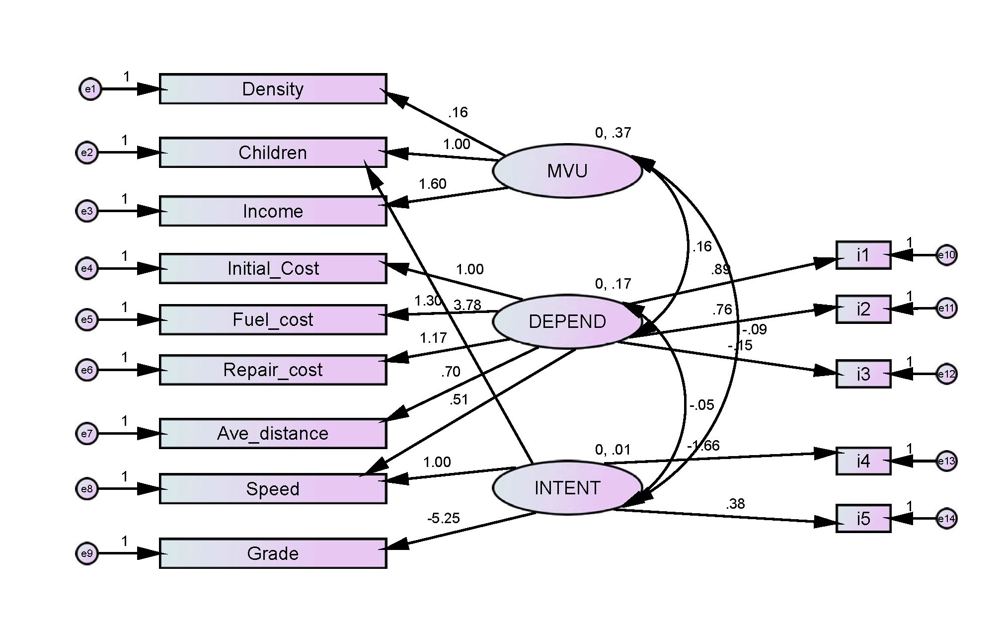
The AMOS output represents the unstandardized and standardized regression coefficients. Figure 1 shows the unstandardized factors loading and measurement of the three latent variables by unstandardized estimates method.

Each unstandardized regression coefficient represents the amount of alternate in the established or mediating variable for every one-unit change in the variable predicting it (The Division of Statistics + Scientific Computation, 2012). The unstandardized coefficients and associated test statistics named “Regression Weights”.

Figure 1. Unstandardized estimate of Structural Equation Model (SEM)

Table 15 shows density increases 0.159 and monthly income increases 1.600 for each 1.000 increases in having children. The table shows the unstandardized estimate, its standard error (abbreviated SE), and the estimate is divided by way of the standard error (CR). The probability value related with the null hypothesis that is zero displayed beneath of the P-column. In other words, P-value indicates that the regression weight for MVU in the prediction of density and monthly income are not significantly dissimilar from zero at the 0.05 level (two-tailed).

Similarly, fuel cost, repair cost, average travel distance, speed, i1 and i2 increase by 1.301, 1.166, 0.703, 0.513, 0.888, 0.762 and i3 decrease by -0.153 for each 1.000 increase in initial cost of the motor vehicle. In other words, the regression weight for DEPEND in the prediction of fuel cost and repair cost is significantly different from zero at the 0.001 level (two-tailed). In addition, regression weight for DEPEND in the estimation of average travel distance, speed and i1 are significantly dissimilar from zero and for DEPEND in the estimation of i2 and i3 are not significantly dissimilar from zero at the 0.05 level (two-tailed).

In addition, social grade and i4 decrease by -5.253 and -1.662 and having children and i5 increase by 3.784 and 0.379 for each 1.000 increases in vehicular speed of the motor vehicle. In other words, the regression weight for INTENT in the estimation of social grade is significantly dissimilar from zero at the 0.05 level (two-tailed) and the regression weight for INTENT in the estimation of having children; i4 and i5 are not significantly dissimilar from zero at the 0.05 level (two-tailed).

Above all gives the overview of significance of different factors with three different latent variables. Due to MVU, there is no significant factor influencing the latent variable. Besides, in case of DEPEND, there are some factors such as average travel distance and vehicular speed significantly affect the latent variable as well as i1 (means owner’s lifestyle depends on having motor vehicle) also significantly influences the dependency latent variable named DEPEND whereas i1 acts as indicator of DEPEND variable. Furthermore, in case of INTENT, social grade influences significantly and because of social grade, respondent doesn’t have intention to reduce motor vehicle uses.

Standardized estimates permit to evaluate the relative contributions of each observed variable to each product as well as latent variable (The Division of Statistics+Scientific Computation, 2012).

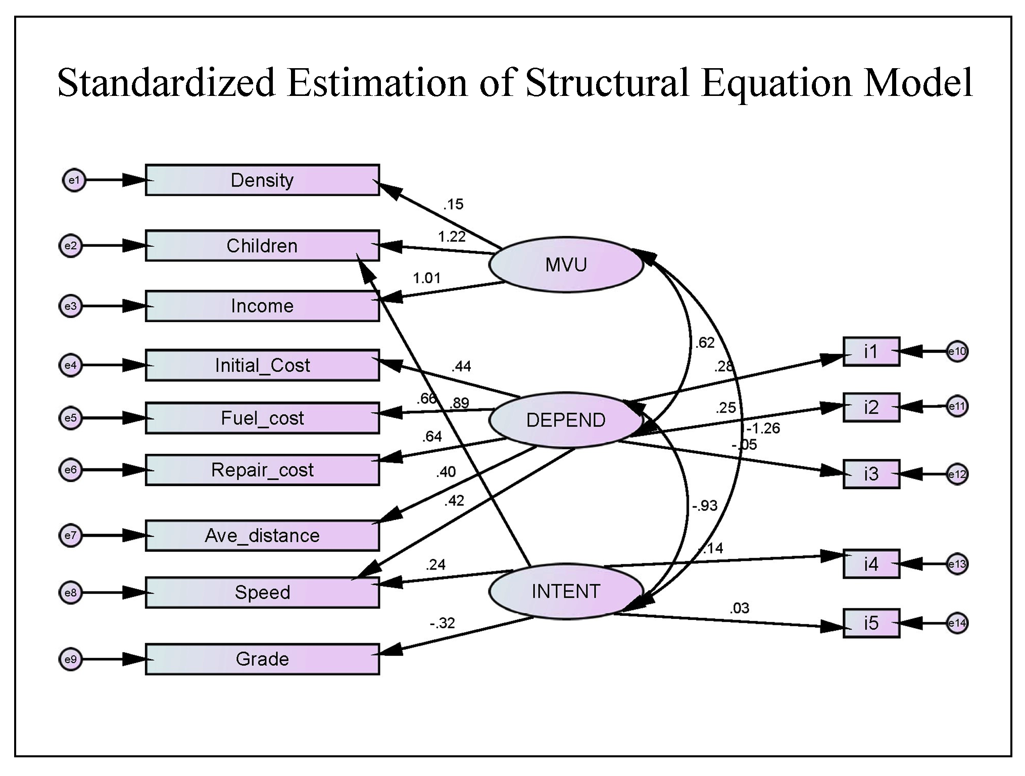
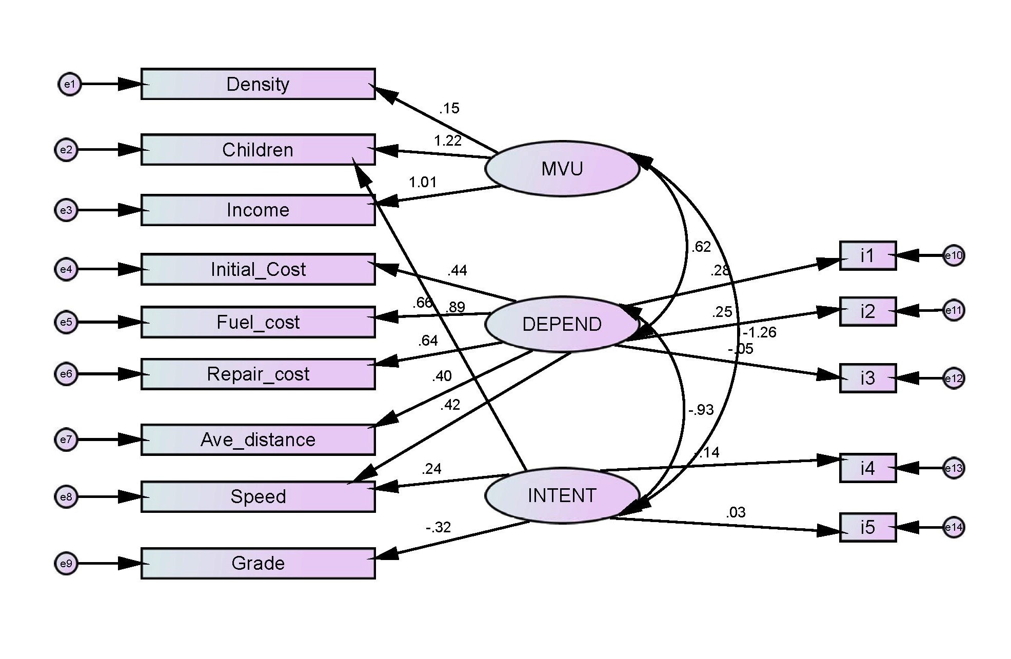
Figure 2 shows the standardized path relation between the observed variables and latent variables. The regression coefficients are called “Beta Weights”, if the predictors and criterion variables are standardized.

Figure 2. Standardized estimate of Structural Equation Model (SEM)

When there is single predictor, a beta weight equal to the correlation. But, if there are two or more predictors available, a beta weight can be larger than +1 and smaller than -1. To understand the regression weights between variables more precisely, table 8 is given below.

The following table describes the regression weights estimated between observed and latent variables. Three different observed variables such as density, having children and income influence the latent variable MVU. Children and income have large influence of motor vehicle use as the beta weights are 1.22 and 1.01 which are greater than 0.8. Besides, density of the living area has small influence of MVU as the beta weight is 0.152 which is less than 0.5. In case of DEPEND variable, fuel cost and repair cost have moderate influence of motor vehicle dependency as the values are 0.66 and 0.65. If the beta weights are situated in between 0.5 to 0.8, then the variable should have moderate influence on the latent variable. Initial cost, average travel distance, speed, i1 and i2 have small influence as the weights fall down in between 0.5 to 0.2. Furthermore, i3 has very small as well as no influence on dependency of motor vehicle as the beta weight is -0.046 as the value is less than 0.2.

In addition, in case of the latent variable INTENT, only having children has large influence as the beta weight is 0.895. If better alternative eco-friendly vehicle is available, then the respondents having children are intended to reduce motor vehicle use for reducing environmental pollution. On the other hand, speed shows small influence and grade, i4 and i5 have no influence on intention to reduce motor vehicle use.

Squared Multiple Correlation (SMC) indicates a squared multiple correlation or R2 for the regression equation suggests the share of variance in the dependent variable accounted for by way of the set of independent variables in the multiple regression equation. The squared multiple correlation reports the relation between each endogenous variable and the variables (other than residual variables) that directly affect it. Say for example, in the table, estimated value of density is 0.23 (Table 16) which means that predictors of density MVU explain 2.3% of its variance. Besides, the error variance of density is approximately 97.7% of the variance of density itself. Similarly, income shows greater value which indicates the predictor of income MVU explains 102.9% of its variance. Hence, income affects greater than all other variables in case of MVU.

Furthermore, the predictor of repair cost and fuel cost DEPEND explain 41.6% and 43.4% of its variance. In addition, the error variance of repair and fuel costs are approximately 58.4% and 56.6% of the variance of repair cost and fuel cost. Estimated value shows that both have a greater influence of dependency of motor vehicle as the estimated value is greater.

Lastly, the estimated value of social grade is 0.1 (Table 17) which means the predictors of grade INTENT explain 10% of its variance and the error variance of grade is approximately 90% of the variance of grade itself. Estimated value of having children indicates that the predictors of children MVU and INTENT explain 46.8% of its variance and the error variance of children is approximately 53.2% of the variance of children itself.

Correlations indicate the mutual relationship or connection between latent variables. Table 18 shows the mutual correlation among MVU, DEPEND and INTENT.

Correlation value between MVU and DEPEND is 0.621 that means motor vehicle use positively related to the motor vehicle dependency. Motor vehicle dependency increases due to increment of motor vehicle uses. Besides, correlation between DEPEND and INTENT indicates the value -0.928 which is negatively correlated and that means people do not want to reduce motor vehicle use as they are dependent on motor vehicle use. In fact, correlation between INTENT and MVU is -1.3 which is also negatively correlated and that means people frequently use motor vehicle and not intended reduce motor vehicle.

4 . CONCLUSION AND RECOMMENDATIONS

Though urbanization spreads globally, traffic, mobility and transportation related issues have become a challenging issue for developing country. Rapid dependency on individual motorized vehicle makes the whole transportation system congested, causes uncontrolled traffic jam and pollution. To solve this, issue many research and policies are taken place in different time. The study introduces new measures along with traditional measure with excellent statistical relationships between variables that are easily interpreted. The reasons why this measure is necessary are given below.

1. The study analyzes the subjective car dependence which carries respondent’s psychological state of feelings and these feelings can be transformed as a measurer.
2. SEM is the actual model which analyzes the psychometric data to quantify subjective car dependence.
3. Statistical linkage between latent variables can easily be quantified through this model.
4. SEM helps to identify the intention to reduce motor vehicle use statistically from psychometric data which can help us to give weightage of this concept.

The first objective describes the traditional method to analyze the affecting factors behind this motor vehicle dependency and then using these factors by SEM modeling statistical link between the variables and the significant effects are calculated using the second objective. The key outcomes of the study are:

1. First objective identified the affecting factors such as population density of living place, monthly income, having children, initial cost of motor vehicle, fuel cost, repair cost, average travelling distance, speed and social grade which are affecting motor vehicle use, dependency and intention. 
2. Three latent variables MVU, DEPEND and INTENT are assumed with the linking of above factors. Five indicators are also used to measure DEPEND and INTENT.
3. The model explained the first hypothesis which is MUV affects positively with DEPEND and both negatively affect INTENT. Hence, these have causal relationship which describes the correlation between variables.
4. Unstandardized estimate shows that using having children as unit variable, no influencing factors have been found. On the other hand, in case of standardized estimate, children and monthly income have large influence. Beta weigh shows the influencing weight of the observed variables and these are 1.22 and 1.01, respectively. 
5. In case of DEPEND, unstandardized estimate shows that fuel cost, repair cost, average travelling distance and speed are significant for dependency on private motorized vehicle. Indicator i1 shows better influence on DEPEND. On the other hand, in case of standardized estimate, fuel cost and repair cost moderate influence on dependency as the beta weights are 0.66 and 0.65, respectively. R² indicates that the predictor of repair cost and fuel cost DEPEND explain 41.6% and 43.4% of its variance. In a word, as the fuel cost and repair cost are less (in case of motor bike); these factors show greater significance on dependency.
6. Furthermore, social grade is the most significant factor for MVU in unstandardized estimate method. The more the grade is, the less intention to reduce motor vehicle use. In addition, estimated value of i4 shows negative value as people are not actively trying to use motor vehicle less. In case of standardized estimation, having children shows large influence as the respondent having children are indented to reduce motor vehicle use for environmental safety if there is a practical alternate eco-friendly vehicle available. In case of squared multiple correlations, the predictors of grade and having children MVU and INTENT explain 10% and 46.8% of its variance. So, it is clear that social grade and having children are the influencing factors for intention to reduce motor vehicle use.

Correlation values indicate that, due to increase of motor vehicle use, the dependency rate is also increasing but intention to reduce motor vehicle use is gradually decreasing. 

Due to increase of motorized vehicle users, the transportation sector faces sever uncontrolled problems. So, to take control over transpiration sector, it is recommended that emphasis more precisely on the research realizing the affecting factors, authority can emphasis the affecting factors and can serve alternate approaches to minimize this problem. Furthermore, for new urban planning and transportation planning approaches, integrating eco-friendlier, safe and convenient approaches, and concerned authority can move towards more sustainable transportation practices and behaviors. Finally, additional research will be focused on the people who have selected to live and invest their future cities to build an enhanced sustainable urban issue.

Tables

Figures

Conflict of Interest

Acknowledgements

Abbreviations

References