1 . INTRODUCTION
A forest is a community of living organisms which interact mutually with the physical environment. Forest covers approximately 30% (Carlowicz, 2012) to 31% (FAO, 2015) of the earth surface with complexities and self-regenerating capacities (Bauer et al., 1994; Virk and King, 2006; Healey et al., 2008). It is a source of organic carbon, which helps to maintain planetary climate, freshwater, biodiversity and useful to manage hazards like soil erosion, landslides, floods, etc. They are habitat of wildlife and regulate different cycles including hydrological, nutrient, atmospheric, etc. and conserve soils, water, etc. (Southworth, 2004).
Land under natural forest is estimated about 33.36 million km² (World Resources Institute [WRI]) to 39.88 million km² (World Conservation Monitoring Centre [WCMC]) excluding marine forests (Mishra et al., 2003; Kumsap et al., 2005; Fettig et al., 2007; Forkuo and Frimpong, 2012). However, from last some decades forest destruction and land appropriation increase, globally (Turker and Derenyi, 2000). Land under forest in India declined to 21.31% of Total Geographical Area (TGA) (ISFR, 2009 and FSI 2015) due to imbalance climatic conditions, soil degradation, deforestation, desertification and water stresses in drought conditions. India endowed with an immense variety of forest resources (Southworth, 2004). However, adverse changes in ecosystem are taking place with continuous pressures of an exploding population and the subsequent domestic needs including food, fuel, fodder, timber as well as industrial demands (Keenan et al., 1999). There are significant losses of forests at an alarming rate (Pant et al., 2000; Hayes and Sader, 2001). The ‘hotspots’ are identified and declared for tropical biodiversity in Western Ghats. These regions are house of rich biodiversity and globally endemic species (Fang and Xu, 2000). However, it is widely believed that the natural vegetation in this tropical region is losing the biodiversity at unprecedented rates (Panigrahy et al., 2010). Around, 275 million rural people (27%) in India are depends on forests for their subsistence and livelihoods (Kim et al., 2011), earning from trade of fuel wood, fodder, bamboo and minor forest products. It is notable that 17% of rural population in India depends on forests to meet their domestic energy (Drescher and Perera, 2010).
Governmental and non-governmental agencies are involved in conservation of forests from last some decades (Cohen et al., 1998). Planning and management for conservation of forest demands reliable information, investigation and analyses (Cohen et al., 1998; Hansen et al., 2000, Hayes and Sader, 2001; Bhagat, 2009). Many analysts have reported sophisticated techniques like remote sensing (Kennedy et al., 2009), geographic information system (Healey et al., 2008), global positioning system along with mathematical and statistical methods (Fettig et al., 2007) for change detection. Estimations of forests cover using satellite data can give satisfactorily results (Cano et al., 2006). Furthermore, change detection analysis can provide analytical data about forest degradation and conservation (Pouliot et al., 2002). However, reliable change detection techniques for forests using remote sensing data remains a challenging task (Coppin et al., 2004; Im et al.,2008; Schwilch et al., 2011; Sommer et al., 2011; Bhagat, 2012). The results are susceptible to data quality, technical efficiency and suitability of selected techniques (Bhagat, 2012). Therefore, modified change detection technique designed for this study based on field checks and statistical analyses to get more precise analysis about forest changes (Southworth, 2004). The Landsat-5 TM and Landsat-7 ETM+ datasets have been used for detection of changes in forest cover in the study area. Two approaches have been adopted for this analysis: Approach I) post-classification technique and Approach II) improved post-classification technique (Chandio and Matori, 2011). Changes in forest were detected using post-classification techniques using NDVI (Fettig et al., 2007) calculated for Landsat-5 TM and Landsat-7 ETM+ datasets, whereas normalized indices and coefficients were used for improved approach of change detection.
Change detection analysis provides a thematic views to understand the natural and artificial behaviour of changes in land (Sommer et al., 2011) including 1) increase and decrease in area, 2) seasonal changes in forests, snow cover, coastline, ocean water, 3) mapping of floods, landslides, volcanic eruptions, corral rifts, wild animals, birds, 4) changes in near surface atmospheric conditions like temperature, snowfall, rainfall, clouds, fog, storms, and 5) human activities like military actions, observation, planning and management for war areas, coal mining, etc. (Lunetta et al., 2006). Scientists have used different methods of Digital Change Detection (DCD) including classification of multiband satellite data based on image ratio, tasseled cap coefficient, spectral vegetation indices, principal component analysis, change vector methods, threshold based classification, post-classification comparison, univariate image differencing, simultaneous analysis of multi temporal data, fusion approach, spectral classification, algebraic methods, regressions, etc. (Petit and Lambin, 2001; Bhagat, 2012). However, all methods are not ideally suitable, reliable and applicable to all surface change conditions (Du et al., 2002; Bhagat, 2012). Therefore, corrective measure has been suggested to achieve more precise results of forest change detection in this study. Correlation techniques have been used to find the suitable parameter for corrections from different multiband ratios (Coppin and Bauer, 1996) and spectral indices (Huete et al., 2002). Here, correlation and regression (Mountrakis et al., 2010) techniques have been used to determine variables for detection, estimations of exaggerations and corrections using information collected for stable land surface (water bodies, rocky lands, deep forest, etc.). The suggested technique for forest change detection can be useful for land management and especially forests.
4 . METHODOLOGY AND APPROACHES
Two approaches were used for detection of changes in forest cover: Approach I - post classification technique and Approach II - improved post-classification technique. Accuracy assessment was performed and results of analyses compared to check the applicability of the approaches. Statistical techniques were useful to inculcate robustness in the analysis for change detection (Theiler and Perkins, 2011).
4.1 Co-registration
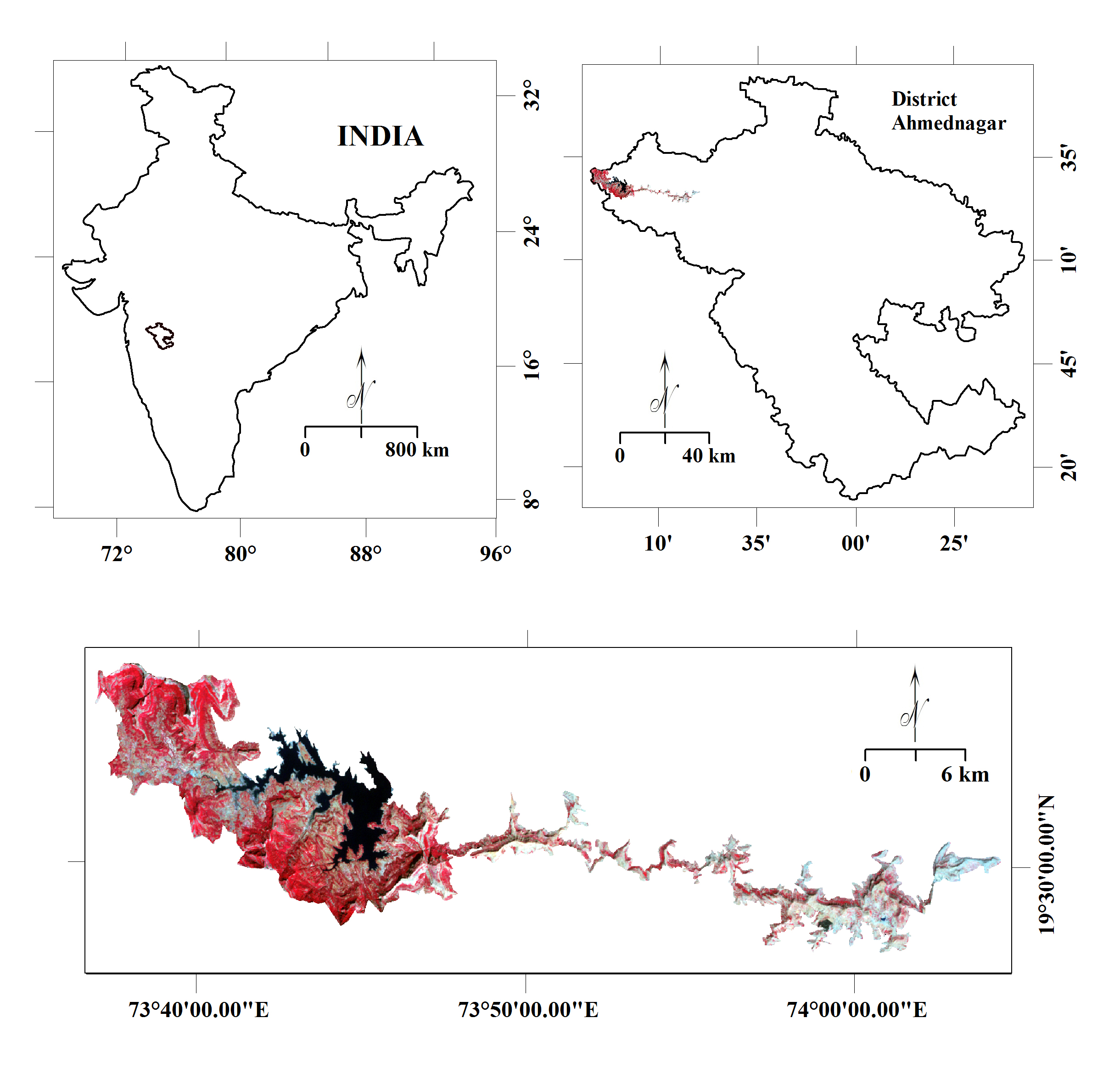
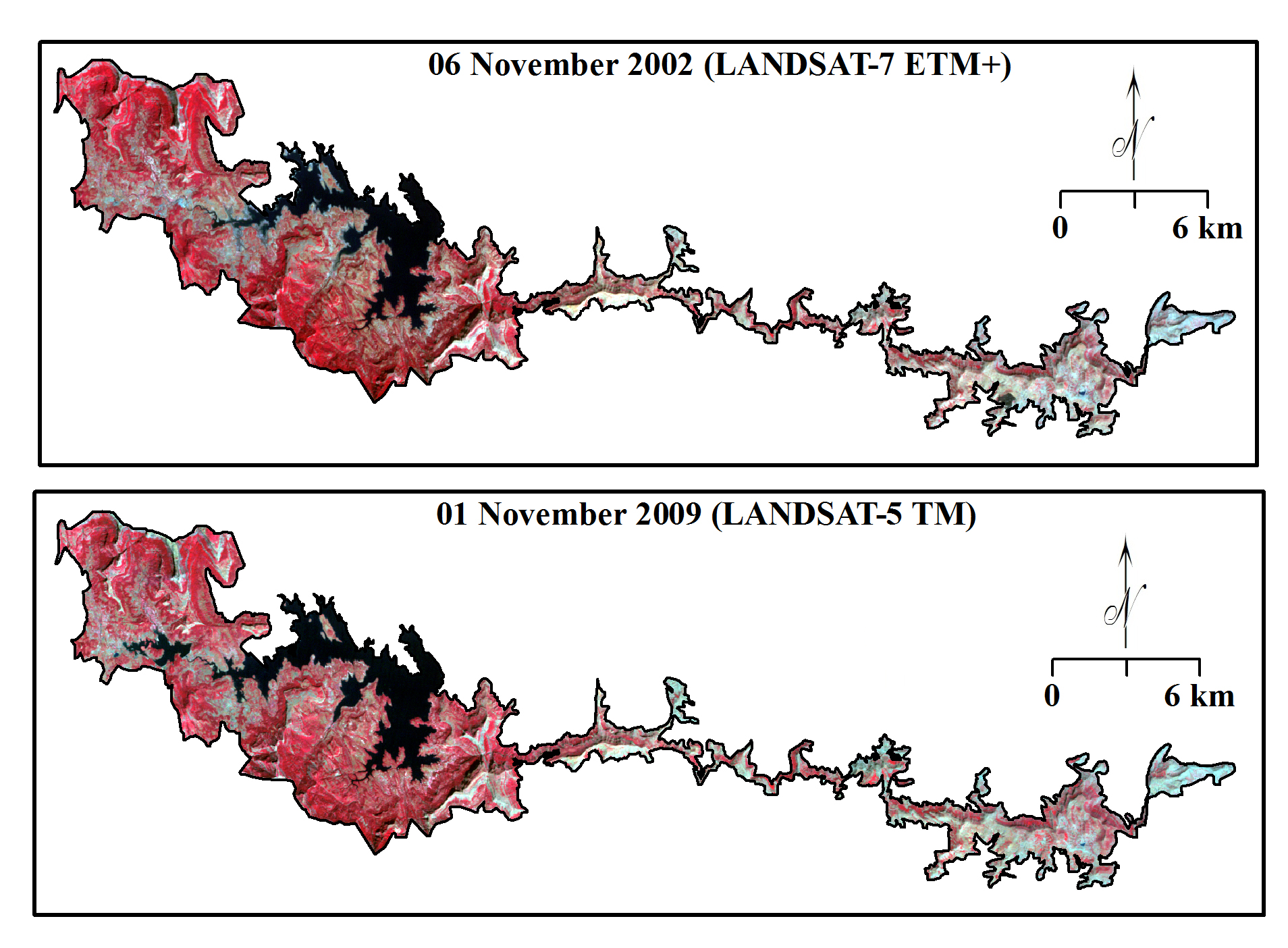
Matching of multiple images captured at different time is critical task for change detection studies. Mis-registration of images drops accuracy in results obtained in change detection analysis (Burnicki et al., 2010; Bhagat, 2012; Pajares et al., 2012). Authors such as Giri Babu et al., (2014) and Tsai and Lin (2007) have suggested automatic tie point registration, pixel to pixel matching, ground control point registration, semi-automotive registration, etc. to obtained reliable results (Clifton 2003; Julien et al., 2011). Therefore, Landsat-7 ETM+ (t1) (2002) and Landsat-5 TM (t2) (2009) scenes were co-registered with the help of: 1) ground truth information (Hara et al., 2012) collected using Garmin GPS device and 2) topo-maps (Survey of India) with pixel to pixel match with 0.00012 Root Mean Square Error (RMSE) in ERDAS Imagine software.
4.2 Image Enhancement
Scientific understanding of behaviour and functioning of vegetation landscape, using remotely sensed data with different spectral, radiometric, temporal and spatial resolutions, have been important task in last some decades (Lippitt et al., 2011; Schwilch et al., 2011). Enhancement of images selected for analysis is highly required before further applications like classifications, estimations, etc. (Chowdhury et al., 2005; Weng et al., 2009; Ehlers et al., 2010). Vegetation indices like NDVI, LAI, TVI, etc. (Silleos et al., 2006) have been calculated using different bands e.g. red, infrared, thermal infrared, middle infrared and widely used for detection of land objects. Furthermore, coefficients like Soil Wetness Index (SWI), Normalized Difference Salinity Index (NDSI), Brightness, etc. have been used to study the distribution of soil moisture, soil salinity, etc. Spectral indices viz. NDVI, LAI and Land Surface Temperature Index (LSTI) and Tasseled Cap Coefficient Transformation have been calculated for enhancement of satellite images in present study.
4.2.1 Spectral Indices
In present study, Difference Vegetation Index (DVI), Ratio Vegetation Index (RVI), NDVI, Soil Adjusted Vegetation Index (SAVI), Leaf Area Index (LAI), Ratio Difference Vegetation Index (RDVI), Modified SAVI (MSAVI), Infrared Percentage Vegetation Index (IPVI) and Modified Simple Ratio (MSR) (Mróz and Sobieraj, 2004) have been used for change detection analysis. However, NDVI has been widely used for detection of changes in forest cover (Bhagat, 2012). Therefore, NDVI (equation 1) has been calculated using Near Infrared (Band 4) and Red (Band 3) bands of Landsat-7 ETM+ and Landsat-5 TM sensors (Bhagat and Sonawane, 2010).
\(NDVI = {NIR-RED \over NIR+RED}\) (1)
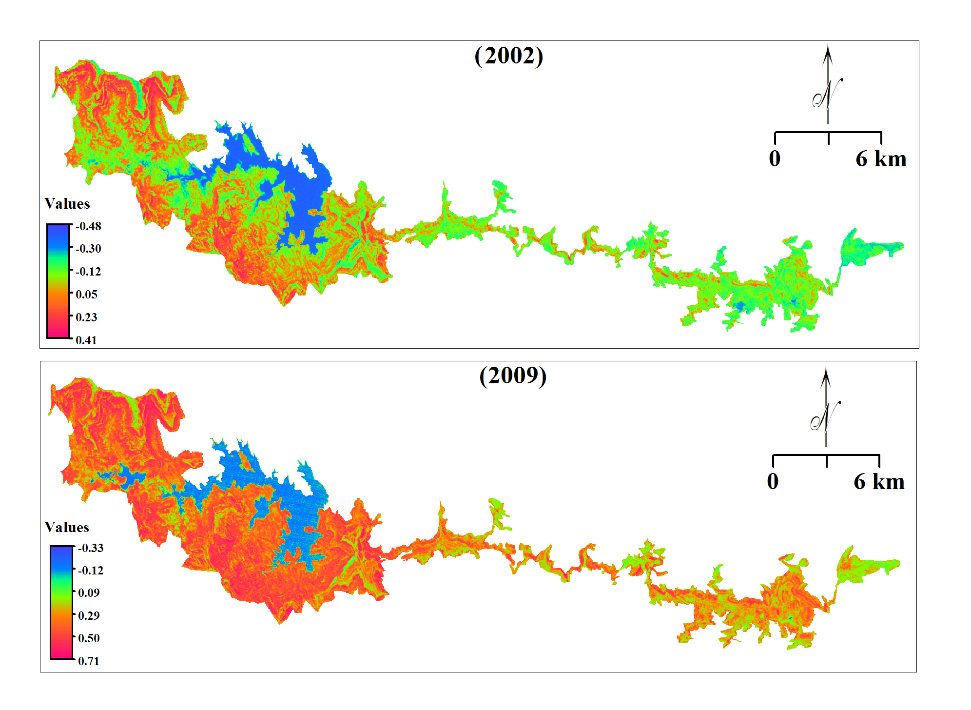
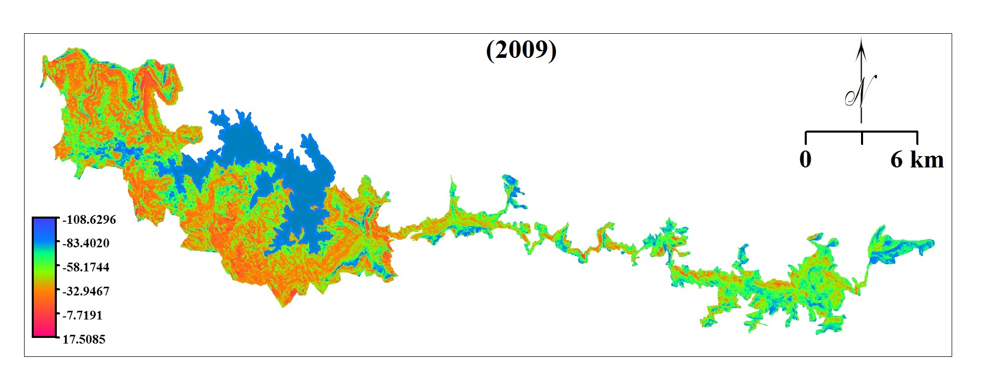
Calculated NDVI values vary between -1 to +1 depending on relative Digital Number (DN) of Near Infrared and Red bands. Maximum NDVI (Figure 2) indicates dense vegetation and minimum values represent less or absence of vegetation.
Leaf Area Index (LAI) [m2/m2] represents the amount of leaf material in an ecosystem and is geometrically defined as the total one-sided area of photosynthetic tissue per unit ground surface area (Breda, 2003; Jonckheere et al., 2004; Morisette et al., 2006). It appears as a key variable in many models describing vegetation-atmosphere interactions, particularly with respect to the carbon and water cycles (GCOS, 2010). LAI was calculated using following equation after Jensen (2002) (equation 2):
\(LAI = -2.42 +12.18 *(NDVI)\) (2)
Where, -2.42 and 12.18 are the constants (Jensen, 2002). LAI is widely used to identify and delineate light interception, gross productivity, soil moisture and transpiration from vegetation (Chen et al., 2012). Therefore, LAI were calculated for statistical analysis to test applicability for Forest Change Detection (FCD) in second approach. Furthermore, many scholars have been used Land Surface Temperature Index (LSTI) for vegetation analysis (Yuan and Bauer, 2007). LSTI is measurements of earth surface temperature including canopy, soils, barren lands, rocks, water bodies, snow, ice, roof of a building using satellite data. The DN recorded for satellite images (Julien et al., 2011) were converted (equation 3) using space reaching radiance i.e. Top of Atmosphere (ToA) Radiance (equation 4) (Chander and Markham, 2003).
\(LST(T) = {{K_2} \over in({k_1\over L_\lambda}+1)}\) (3)
Here, \(T\) is an effective at-satellite temperature in k (kelvin), \(L_\lambda\) is a spectral radiance in W/(m2 in µm), \(K_1\) and \(K_2\) are pre-launch calibration constants for ETM+ and TM sansors.
\(L_\lambda = ({{L_{max}-L_{min}} \over QCAL_{max}-QCAL_{min}})(DN-QCAL_{min})+L_{min}\) (4)
Where, \(L_{max}\) is a maximum spectral radiance (W/m2 in µm) at QCAL equal 0 DN, \(L_{mim}\) is a minimum spectral radiance (W/m2 in µm) at QCAL equal 255 DN and QCAL are the quantized calibrated pixel values in DN.
4.2.2 Tasseled Cap Coefficient Transformations (TCCTs)
TCCTs have potentials to derive forest attributes for different regional applications where, atmospheric noise correction not possible (Silleos et al., 2006; Ghosh et al., 2010). These transformations simply reduce the number of radiance noise density and provide high association in single response. Therefore, brightness, greenness, wetness, fourth, fifth and sixth indices were calculated using coefficients estimated by Crist et al., (1986) for Landsat-5 TM (Table 1) and Huang et al., (2002) (Table 2) for Landsat-7 ETM+.
Table 1. Landsat-5 TM: tasselled cap coefficients at satellite reflectance
|
Index
|
Band1
|
Band2
|
Band3
|
Band4
|
Band5
|
Band7
|
|
Brightness
|
0.2909
|
0.2493
|
0.4806
|
0.5568
|
0.4438
|
0.1706
|
|
Greenness
|
-0.2728
|
-0.2174
|
-0.5508
|
0.7221
|
0.0733
|
-0.1648
|
|
Wetness
|
0.1446
|
0.1761
|
0.3322
|
0.3396
|
-0.6210
|
-0.4186
|
|
Fourth
|
0.8461
|
-0.0731
|
-0.4640
|
-0.0032
|
-0.0492
|
0.0119
|
|
Fifth
|
0.0549
|
-0.0232
|
0.0339
|
-0.1937
|
0.4162
|
-0.7823
|
|
Sixth
|
0.1186
|
-0.8069
|
0.4094
|
0.0571
|
-0.0228
|
0.0220
|
|
Source: Crist et al., 1986
|
Table 2. Landsat-7 ETM+: tasselled cap coefficients at satellite reflectance
|
Index
|
Band1
|
Band2
|
Band3
|
Band4
|
Band5
|
Band7
|
|
Brightness
|
0.3561
|
0.3972
|
0.3904
|
0.6966
|
0.2286
|
0.1596
|
|
Greenness
|
-0.3344
|
-0.3544
|
-0.4556
|
0.6966
|
-0.0242
|
-0.2630
|
|
Wetness
|
0.2626
|
0.2141
|
0.0926
|
0.0656
|
-0.7629
|
-0.5388
|
|
Fourth
|
0.0805
|
-0.0498
|
0.1950
|
-0.1327
|
0.5752
|
-0.7775
|
|
Fifth
|
-7252
|
-0.0202
|
0.6683
|
0.0631
|
-0.1494
|
-0.0274
|
|
Sixth
|
0.4000
|
-0.8172
|
0.3832
|
0.0602
|
-0.1095
|
0.0985
|
|
Source: Huang et al., 2002
|
4.3 Approaches of Forest Change Detection
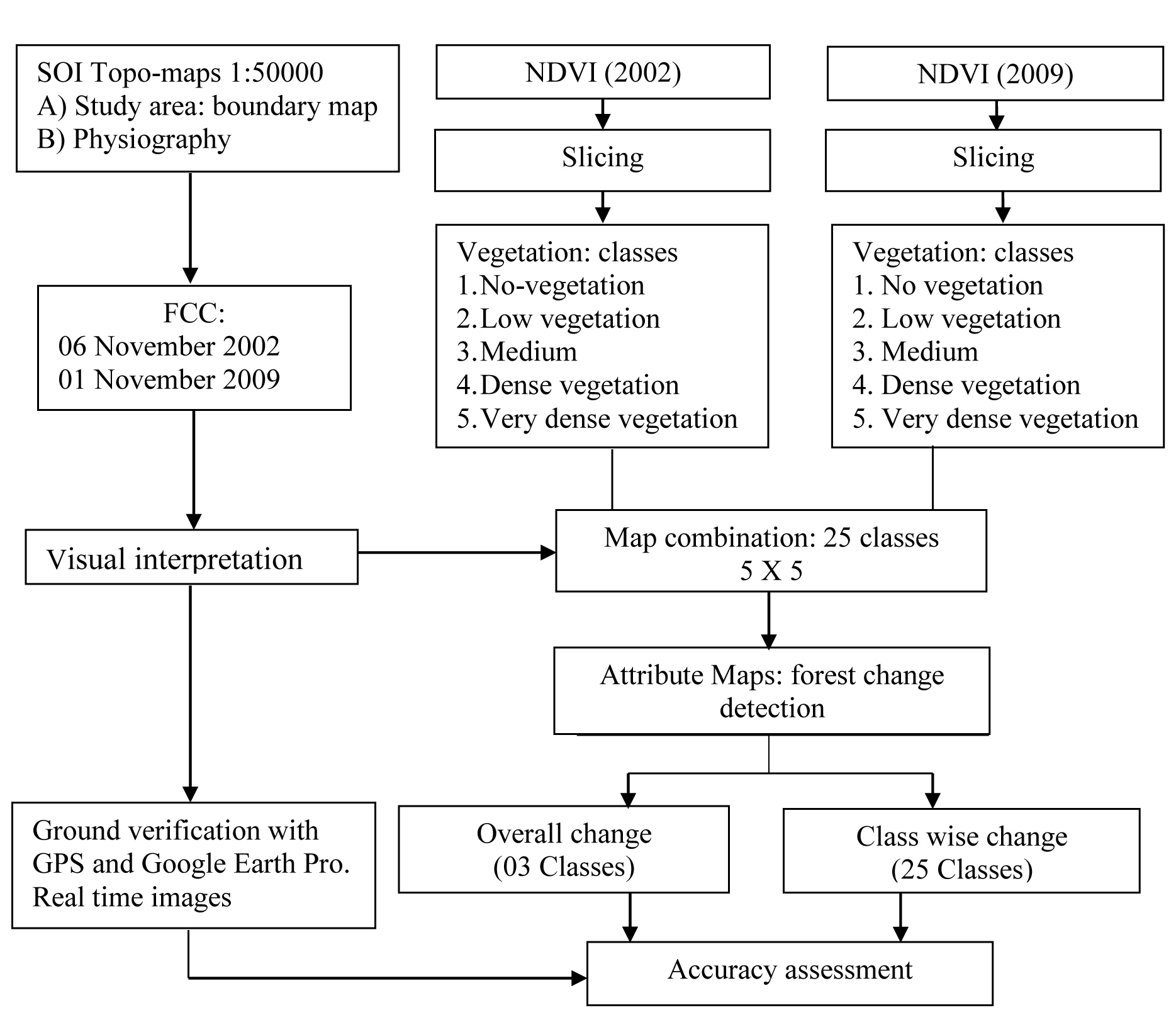
4.3.1 Approach I: Post-classification technique
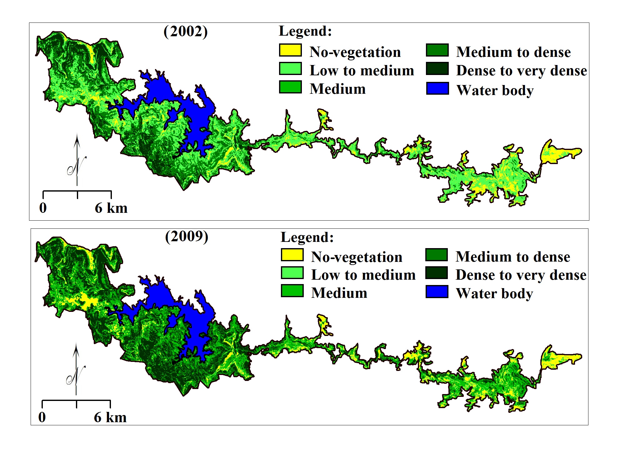
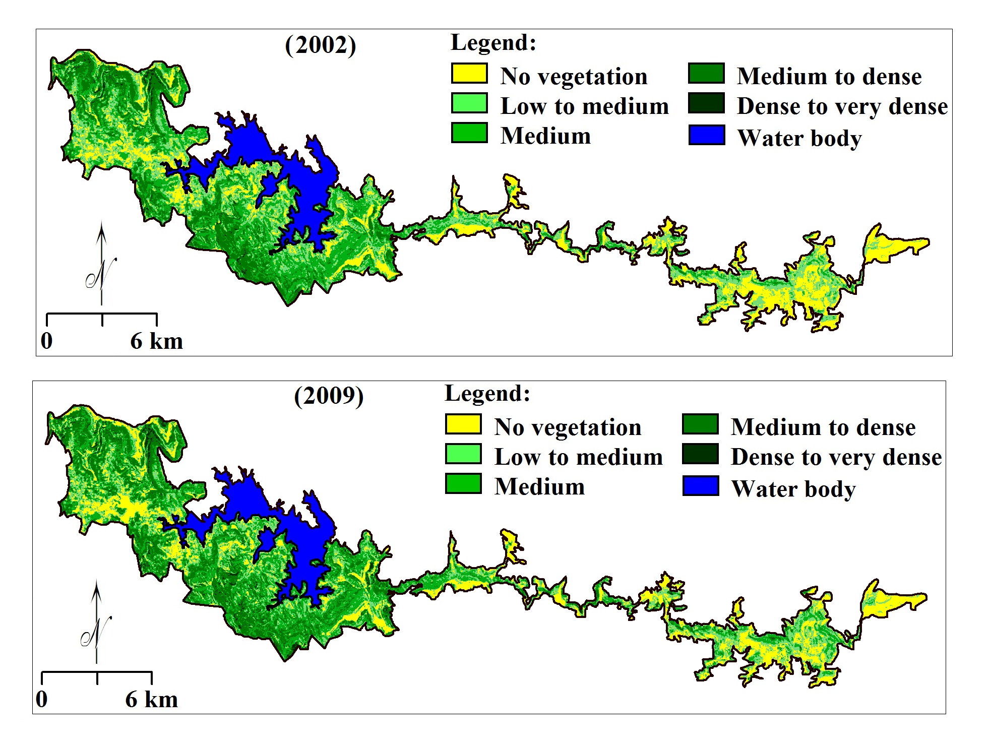
Satellite images selected for present study was processed for co-registration, enhancements, classification and finally, classified images were compared for Change Detection (CD) in forest cover. Calculated pixel values of NDVI have been broadly grouped into five classes (Table 3) i.e. no-vegetation, low to medium, medium, medium to dense and dense to very dense, using threshold observed in NDVI (2002) and NDVI (2009) images using ‘slicing’ operation in Ilwis.
Table 3. Broad classification of forest density based on NDVI
|
Classes
|
Index values
|
|
ETM+ (2002)
|
TM (2009)
|
|
No-vegetation
|
< -0.16
|
< 0.20
|
|
Low to medium
|
-0.16 to -0.02
|
0.20 to 0.23
|
|
Medium
|
-0.02 to 0.01
|
0.23 to 0.36
|
|
Medium to dense
|
0.01 to 0.16
|
0.36 to 0.45
|
|
Dense to very dense
|
0.16 <
|
0.45 <
|
The maximum value (0.41) in reference image (t1) (NDVI 2002) was observed for dense vegetation (Table 3) whereas minimum (-0.48) for barren land including water body, rocky and barren land with 0.05 mean and 0.16 standard deviation. Targeted image (t2) (NDVI 2009) shows the maximum value (0.71) for dense vegetation and minimum (-0.33) for no-vegetation with 0.31 mean and 0.16 standard deviation. Adegoke and Carleton (2002) have been used innovative hybrid image classification technique for change detection analysis of forest. Therefore, limit values of NDVI classes are different for images acquired for 2002 and 2009 (Table 3) and was decided based on repetitive field checks using GPS, comparison with high-resolution images of Google Earth Pro and FCC (Figure 4). Class ‘no-vegetation’ includes rocky and barren lands distributed at higher levels (> 1100 m) of mountain and water bodies at bottom (Figure 3).
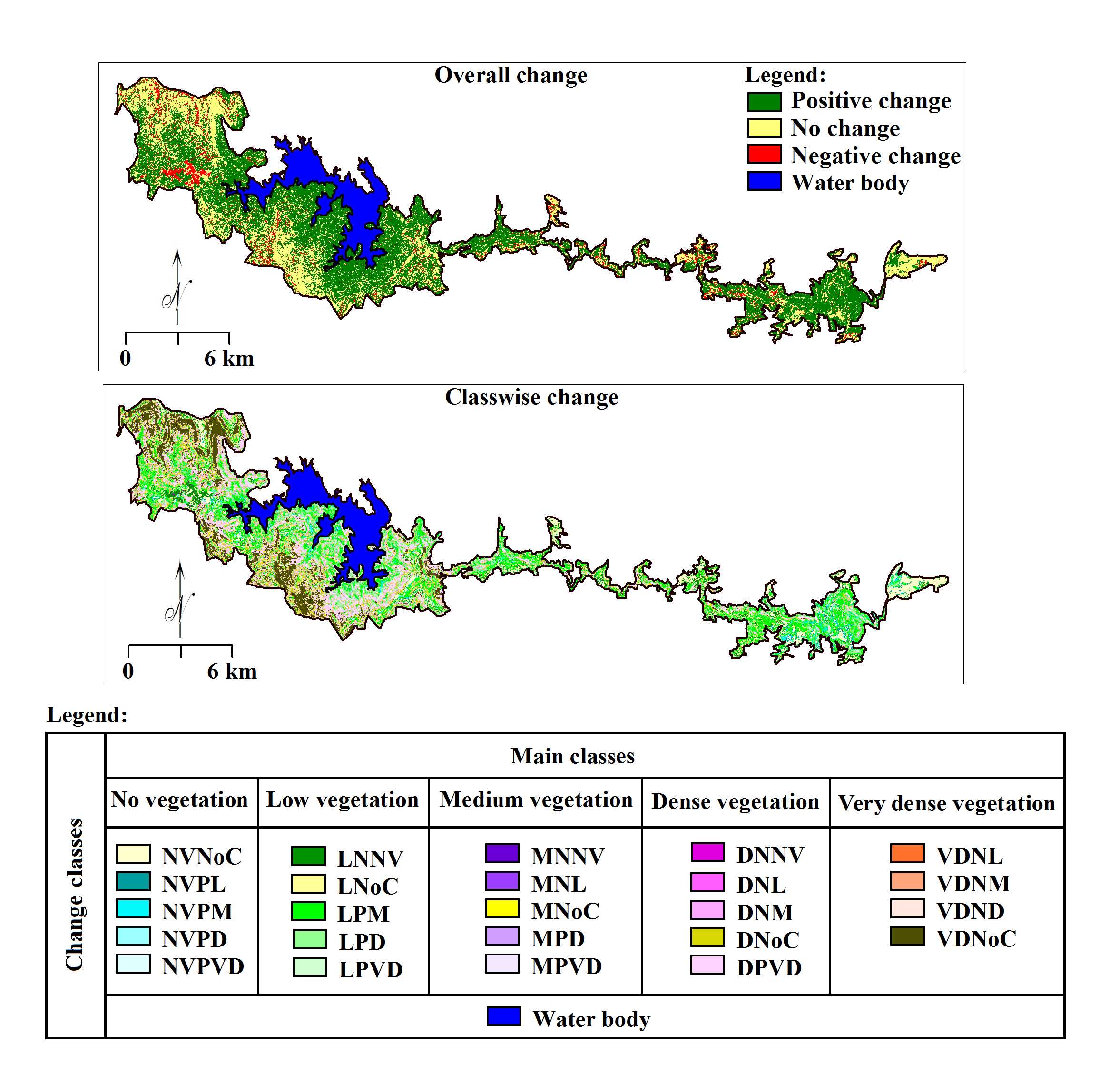
Measurements of differences between detected land classes in base image (t1) and target image (t2) based on radiance difference called change detection (Weng et al., 2009), for instance forest. The radiance difference mainly occurred due to real change in surface features, deviation in atmospheric conditions, deviation in sensor calibration, minimum to maximum error in Route Mean Square (RMS) at the time of georeferencing, deviation in illumination and difference in soil moisture conditions, etc. Here, classified images t1 and t2 combined using ‘cross’ operator (Figure 5) in Ilwis which produce 25 classes (5 classes t1 X 5 classes t2). Similar classes have been merged into three classes viz. no-change, positive change and negative change in forest cover (Table 4) using tool ‘merging the classes’ in Ilwis. Further, class wise changes (Table 11) in forest cover also detected successfully (Figure 14) using same technique (Table 4). However, overall accuracy of the classes detected to show changes in forest cover was estimated about 78%. Users’ accuracy for class ‘positive change’ was about 58% and producer’s accuracy 70%. Rozenstein and Karnieli (2011) have insisted vigorous and creative efforts to establish new algorithms for change detection. Therefore, statistical methods and corrective measures were adopted to achieve improvements in post-classification technique for CD in forest cover.
Table 4. Class merging scheme for overall FCD
|
Vegetation classes: ETM+ (2002)
|
Vegetation classes: TM (2009)
|
|
No-vegetation
|
Low to medium
|
Medium
|
Medium to dense
|
Dense to very dense
|
|
No-vegetation
|
No-change
|
Positive
change
|
Positive
change
|
Positive
change
|
Positive
change
|
|
Low to medium
|
Negative
change
|
No-change
|
Positive
change
|
Positive
change
|
Positive
change
|
|
Medium
|
Negative
change
|
Negative
change
|
No-change
|
Positive
change
|
Positive
change
|
|
Medium to dense
|
Negative
change
|
Negative
change
|
Negative
change
|
No-change
|
Positive
change
|
|
Dense to very dense
|
Negative
change
|
Negative
change
|
Negative
change
|
Negative
change
|
No-change
|
Table 5. Class merging scheme for class wise FCD
|
Vegetation classes:
ETM+ (2002)
|
Vegetation classes: TM (2009)
|
|
No- vegetation
|
Low to medium
|
Medium
|
Medium to dense
|
Dense to very dense
|
|
No-vegetation
|
NVNoC
|
NVPL
|
NVPM
|
NVPD
|
NVPVD
|
|
Low to medium
|
LNNV
|
LNoC
|
LPM
|
LPD
|
LPVD
|
|
Medium
|
MNNV
|
MNL
|
MNoC
|
MPD
|
MPVD
|
|
Medium to dense
|
DNNV
|
DNL
|
DNM
|
DNoC
|
DPVD
|
|
Dense to very dense
|
VDNNV
|
VDNL
|
VDNM
|
VDND
|
VDNoC
|
|
* Refer section- Abbreviations or Table 11 and Table 13 for explanation.
|
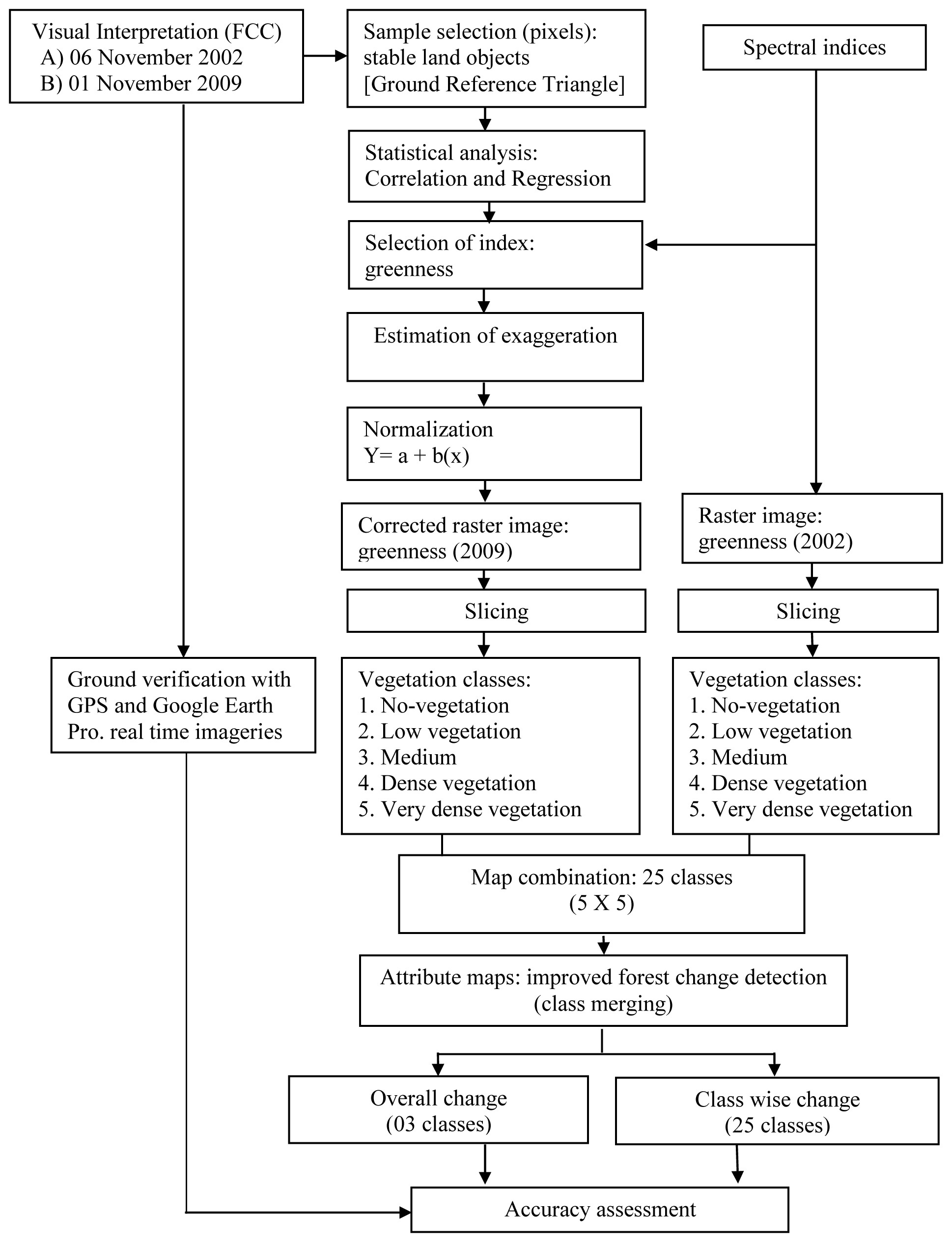
4.3.2 Approach II: Improved post-classification technique
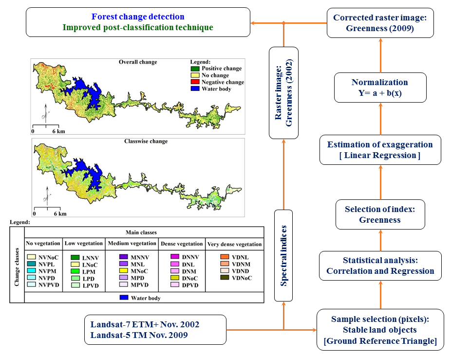
Many scholars have been successfully used combinations of different approaches for CD of land objects (Cano et al., 2006; Pu et al., 2008; Weng et al., 2009). The algorithm of FCD has been modified to improve (Figure 6) the results and processed through five steps: 1) sampling (Chapelle et al., 2002; Lu et al., 2011), 2) statistical analysis (Singh, 1989; Dhakal et al., 2002), 3) normalization of indices, 4) change detection and 5) accuracy assessment. Statistical analysis and information about stable land surface including deep forests, rocky lands, barren lands and water bodies have used for normalization of indices calculated for target image (t2) (Felkar et al., 1981; Singh, 1996; Turker and Derenyi, 2000).
a. Sampling
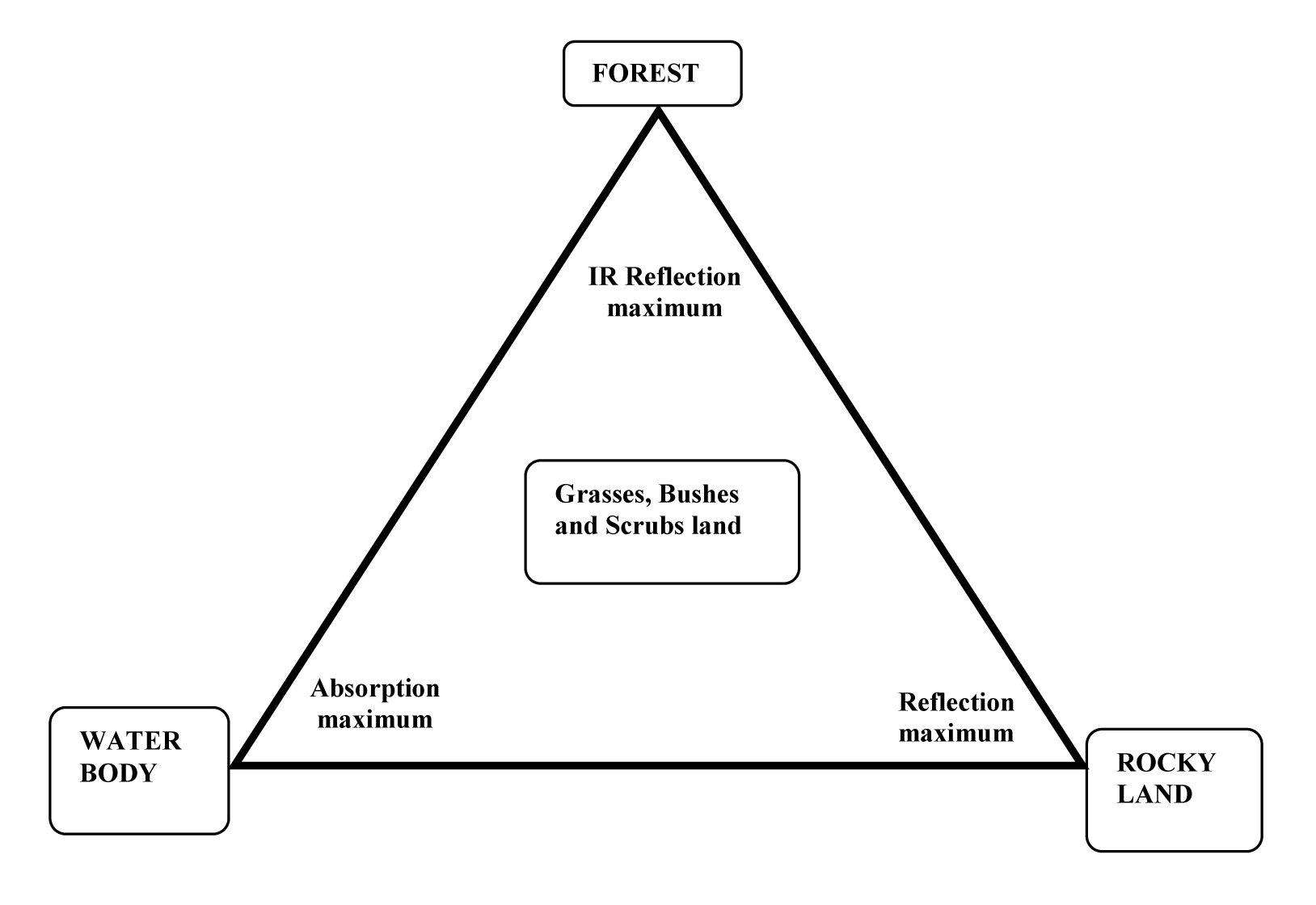
Many researchers have been successfully used single band, ratio indices and coefficients for detection and delineation (Chen et al., 2012) of objects like forests, water bodies, barren lands, rocky lands, snow covers, marsh lands, desert lands, etc. The variations in land phenomenon regulate surface radiance according to their reflectivity (Carlson et al., 1990; Chen et al., 2012). Surface reflectance values are sensitive to variations in vegetation cover, soil, background temperature, thermal inertia, and topography (Bhagat 2012). Goetz (1997) has used inverse relationship between SVI and Ts based on inversion soil-vegetation-atmosphere-transfer (SVAT) model for estimating soil surface moisture using NDVI-Ts triangle space. This approach is defined as the ‘Triangle Method’ includes vegetation indices, soil moisture indices and thermal indices (Weng et al., 2009; Lu et al., 2011). Objects detected using this approach are stood more precise than single bands. Surface temperature can be estimated using thermal band and vegetation can be detected with the help of near infrared band (Nemani and Running, 1989; Carlosan et al., 1990; Nemani et al., 1993; Tanriverdi, 2010). Thus, all surface elements have equal importance in estimations of objects (Owen et al., 1998).
Water body absorbs maximum amount of radiation and emits very little energy (Nemani et al., 1993). Forest cover reflects maximum amount of Green and Near Infrared (NIR) bands and a good absorber of Blue and Red band. Chemical component existing in tree leaves known as ‘chlorophyll’ effectively absorbs radiation from the Blue and Red band (Jiany et al., 2008). The inner structure of these leaves response as good emission of NIR wavelength (Roberts et al., 2011). On the other hand, visible and NIR radiation absorb more in the form of longer wavelength from water body and less from shorter wavelength (Lu et al., 2011). Thus, water appears blue-green or blue due to maximum reflectance of shorter wavelength and viewed dark because reflectance of red and near infrared depending on the suspended sediments amount in water (Fletcher and Everitt, 2007). Rocky lands are purely dry and rarely covered by thin grass and algae in wet seasons. However, rocky lands absorb very low amount of visible as well as NIR waves and reflect maximum as compare to other classes (Majed et al., 2011). Water bodies, deep forests and rocky lands are stable objects and have extreme reflectance (minimum and maximum) in the region.
The variations in reflectance recorded is satellite image have influence on accuracy of forest CD using post-classification (Pu et al., 2008). Therefore, corrective approach was adopted for detection of FCD (discussed in next section). Ground truth information (170 samples) was collected for these stable land objects which were appeared and identified on satellite images e.g. Landsat-7 ETM+ (2002) and Landsat-5 TM (2009). DN values of these land objects were used further statistical analysis and normalisation of indices calculated using satellite data (t2) (Bhagat, 2012). About 31.18% samples were collected from forest cover, 27.65% from rocky land, 29.41% from water body and 11.76% from barren land for further process (Figure 7).
b. Statistical analysis
NDVI has been widely used for vegetation analysis, however, greenness (equation 5 and 6) (Crist et al., 1986; Huang et al., 2002) have more potential of vegetation analysis. Greenness values estimated for both images (t1 and t2) have positively correlated with NDVI. Therefore, greenness estimated for ETM+ (t1) and TM (t2) data was used as dependent variable for estimations corrected greenness values for t2 (Figure 8).
Greenness (ETM+) = ((Band1 * (-0.3344)) + (Band2 * (-0.3544)) + (Band3 * (-0.4556)) + (Band4 * (0.6966)) + (Band5 *(-0.0242)) + (Band7* (-0.2630)) (5)
Greenness (TM) = ((Band1*(-0.2728)) + (Band2*(-0.2174))+ (Band3 * (-0.5508)) + (Band4 * (0.7221)) + (Band5 *(0.0733)) + (Band7 * (-0.1648)) (6)
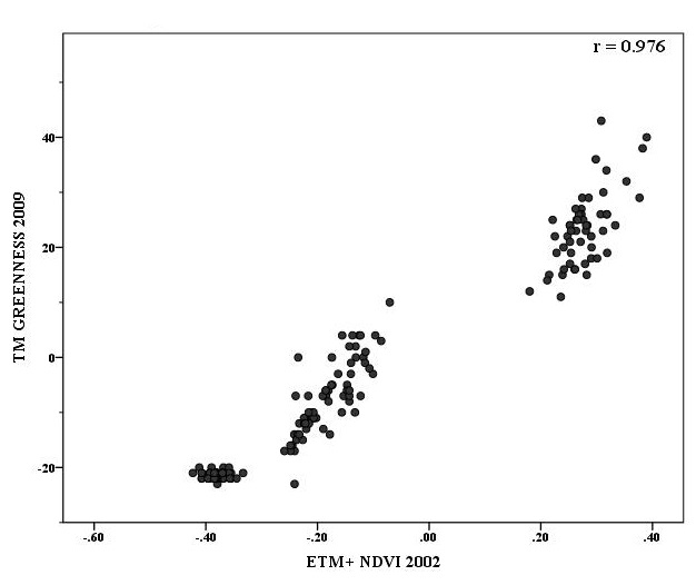
NDVI (2002) values show positive correlation with greenness estimated for t2 (2009) (r = 0.976) and NDVI (2009) with greenness for t2 (2009) (r = 0.975) (Table 6). Scatterplot (Figure 9) for NDVI (2002) and Greenness (2009) show clustered distribution of vegetation. Therefore, calculated greenness values used for estimations of dependent variable in regression analysis. Maximum greenness (-0.07) calculated for t1 (2002) and 65.06 for t2 (2009) whereas minimum (-110.16) for no-vegetation i.e. water, rocky land, shadow, etc. in t1 (2002) and -36.57 in t2 (2009). These are stable land surface in the study area. Theoretically, values estimated for the stable lands might be same which is not possible in certain conditions at the time of image capturing (Munyati, 2004; Yarbrough et al., 2005; Gill et al., 2012). Therefore, accuracy of FCD in the region shows less. Further, these estimated values have been normalized using values estimated for stable pixels in this approach. Differences between estimated greenness values for stable pixels of t1 and t2 have been calculated and correlation with estimated indices SWI (t1), brightness (t1), fifth (t1) and DN values of band 7 (t1), band 7 (t2), band 5 (t1) have been estimated to find independent variables for estimation of normalized dependent variable for t2 e.g. greenness.
Table 6. Correlations between NDVI and Greenness
|
|
Greenness (2002)
|
Greenness (2009)
|
|
NDVI (2002)
|
Pearson correlation
|
0.684**
|
0.976**
|
|
Sig. (2-tailed)
|
.000
|
.000
|
|
N
|
170
|
170
|
|
NDVI (2009)
|
Pearson correlation
|
0.571**
|
0.975**
|
|
Sig. (2-tailed)
|
.000
|
.000
|
|
N
|
170
|
170
|
|
** Significance at the 0.01 level (2-tailed).
|
Significant correlation of calculated difference between greenness estimated for stable pixels of t1 and t2 was estimated with band 7 (t1), SWI (t1), band 5 (t1) band 7 (t2), brightness (t1), difference in SWI, difference in fifth (Table 7). However, the strongest correlation was estimated for band 7 of t1 and therefore this band was used as independent variable for estimations of pixel values of correction in t2 using regression techniques. Samples (170) collected from stable land surface i.e. forest land, rocky land, water, barren land, etc. (Figure 7) was used for this analysis.
Table 7. Correlation of difference greenness with selected criterion
| |
Band7 of t1
|
SWI
of t1
|
Band7
of t2
|
Band5
of t1
|
Brightness of t1
|
Difference
SWI
|
Difference
Fifth
|
|
Difference greenness
|
Pearson Correlation
|
0.983**
|
-0.964**
|
0.960**
|
0.960**
|
0.949**
|
0.934**
|
-0.933**
|
|
Sig.
(2-tailed)
|
0.000
|
0.000
|
0.000
|
0.000
|
0.000
|
0.000
|
0.000
|
|
N
|
170
|
170
|
170
|
170
|
170
|
170
|
170
|
|
** Significance at the 0.01 level (2-tailed).
|
Regression (equation 7) gives mathematical tools (Lawrence and Wrlght, 2001; Cohen et al., 2003) to estimate the fit between two different multi-spectral images acquired at different time for same area. Pixel values close to the regression line indicate the suitability of the model (Table 8).
\(Y=a+b(x)\) (7)
Where, \(Y\) is an estimated variable (dependent), \(a\) and \(b\) are constant ( \(a\) is intercept and \(b\) is rate of change in slope) and \(x\) is independent variable.
Table 8. Regression analysis of difference greenness with selected criterion
|
\(Y\)
|
\(x\)
|
Correlation (r)
|
\(a\)
|
\(b\)
|
R2
|
Trend
|
|
Difference greenness
|
Band7 of t1
|
0.983
|
21.664
|
0.602
|
0.967
|
Positive
|
|
SWI of t1
|
-0.964
|
33.511
|
-0.432
|
0.930
|
Negative
|
|
Band7 of t2
|
0.96
|
24.208
|
0.891
|
0.922
|
Positive
|
|
Band5 of t1
|
0.96
|
20.554
|
0.399
|
0.921
|
Positive
|
|
Brightness of t1
|
0.949
|
-2.307
|
0.370
|
0.901
|
Positive
|
|
Difference SWI
|
0.934
|
30.447
|
0.769
|
0.871
|
Positive
|
|
Difference Fifth
|
-0.933
|
90.231
|
-2.110
|
0.871
|
Negative
|
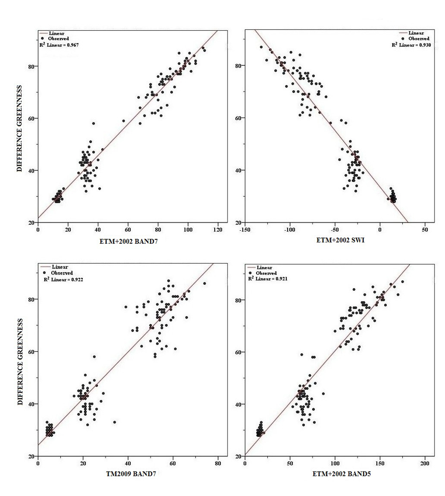
Scholars have been reported the highest change detection accuracy by using regression approach. Jiany et al., (2008) reported three steps of radiometric normalization using pixel values for stable land surface: (1) delineation of stable land based on near-infrared (NIR) bands; (2) DN for stable areas using regression models, and (3) the regression coefficients used for normalizing DN of the target image. Here, linear regression model depicts (Figure 10) the fit (R2= 0.967) of differences in Greenness of t1 and t2 with band 7 of t1 with high correlation (0.983) and clustered distribution. The values closer to zero on x-axis are for water bodies, next cluster for forests and at far from the zero for barren and rocky lands. Band 5 and band 7 of ETM+ and TM images show higher sensitivity to soils and vegetation.
c. Estimation of exaggeration and normalization of images
The maximum value (0.41) in reference image (t1) (NDVI 2002) was observed for dense vegetation (Table 3) whereas minimum (-0.48) for barren land and water body with 0.05 mean and 0.16 standard deviation. Maximum NDVI value (0.71) in target image, (t2) (2009) was observed for dense vegetation and minimum (-0.33) for no-vegetation with 0.31 mean and 0.16 standard deviation. Therefore, it is assumed that the values recorded in target image are exaggerated from ground reality (Figure 8). Regression model (equation 8) was formed to estimate the values of exaggeration in greenness (Ge) estimated for target image (t2) for normalizing (t2).
\(Ge=a+b(B7t_1)\) (8)
Where, \(a\) is an intercept 21.664 and \(b\) is rate of change in slope 0.602 and \(B7 t_1\) is band 7 of reference image (t1). Finally, raster image for greenness estimated for target image (t2) was normalised \(Nt_2\) (equation 9) for final FCD.
\(Nt_2=Greenness2009-Ge\) (9)
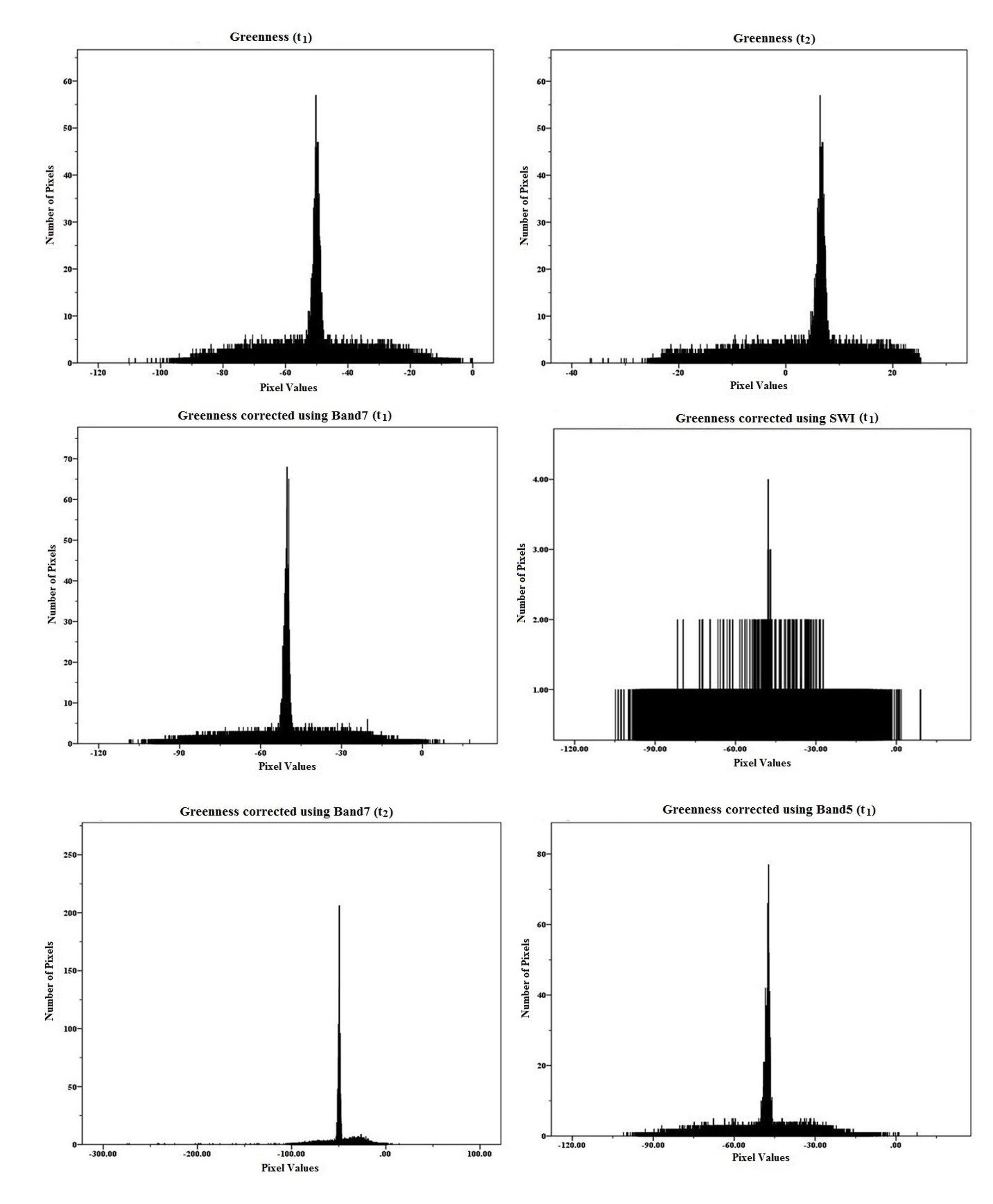
The histograms for estimated images viz. corrected greenness 2009 using band 7 (t1), SWI (t1), band 7 (t2) and band 5 (t1), etc. were prepared in SPSS and compared with histograms prepared for greenness for t1 and t2 (Figure 11). Histogram values distributed from -110.1568 to -0.0782 for greenness of ETM+ (2002) and from -36.5670 to 65.0585 of TM (2009). However, distributed values on histogram prepared for corrected greenness of t2 (2009) vary from -108.6296 to 17.5085. Similar results observed for normalised raster images of band 7 (2002), SWI (2002), band 7 (2009) and band 5 (2002).
4.3.3 Change detection
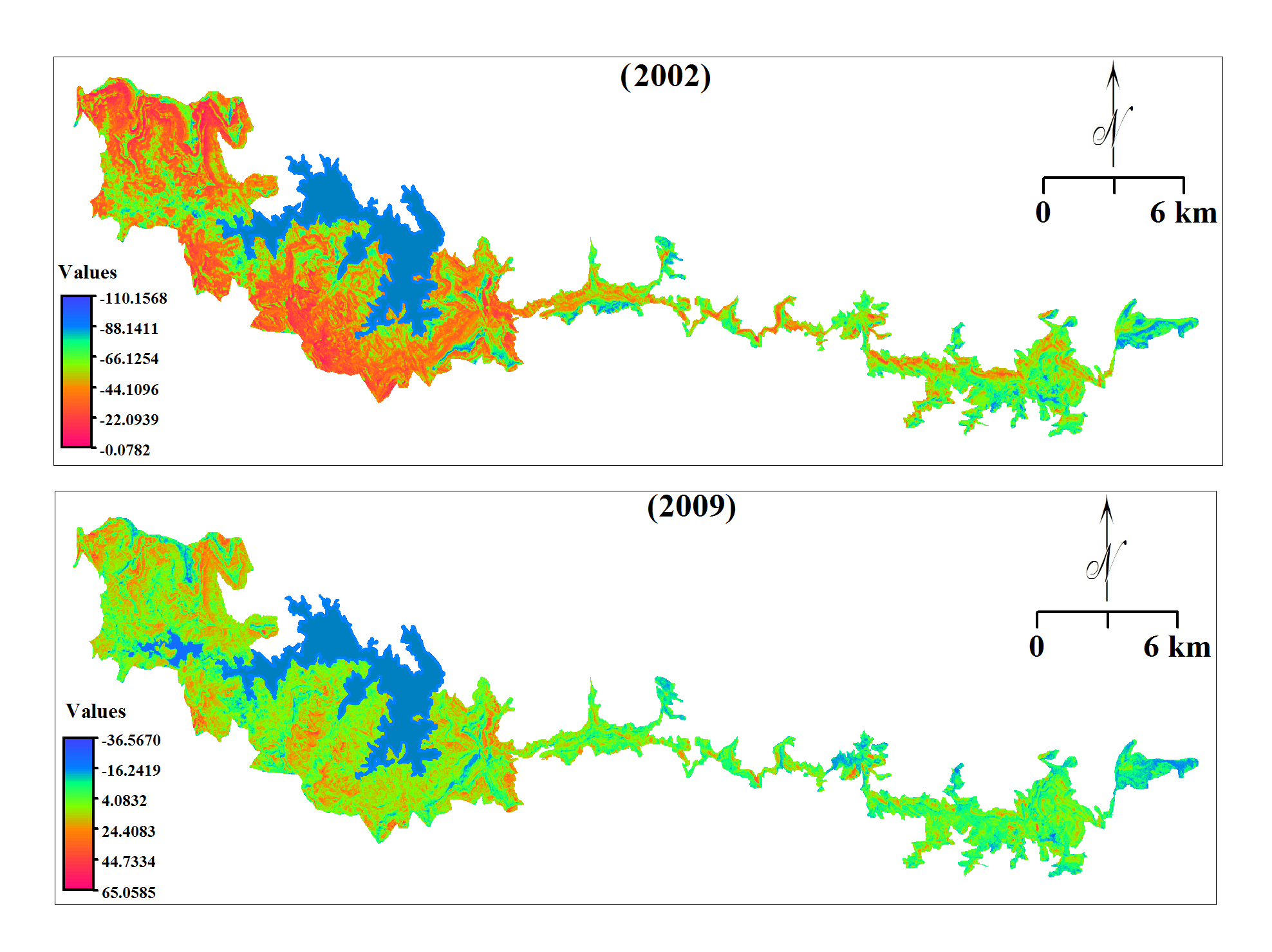
Finally, raster image of greenness estimated for t1 (ETM+ 2002) and normalised raster image of greenness estimated (Figure 12) for t2 (TM 2009) were processed for FCD in this study. The maximum value was -00.08 estimated for greenness of t1 (2002) and 17.51 for normalized greenness (2009) whereas minimum value was -110.16 for t1 (2002) and -108.63 for normalized image t2 for ‘no-vegetation’ i.e. water, rocky land, shadow, etc. (Figure 13). Reference (t1) and normalised (Nt2) images were classified into five classes (Table 9) e.g. no-vegetation, low to medium, medium, medium to dense and dense to very dense, respectively.
Table 9. Broad classification of forest density based greenness index
|
Vegetation classes
|
Index value
|
|
No-vegetation
|
< -64
|
|
Low to medium
|
-64 to -48
|
|
Medium
|
-48 to -32
|
|
Medium to dense
|
-32 to -16
|
|
Dense to very dense
|
-16 <
|
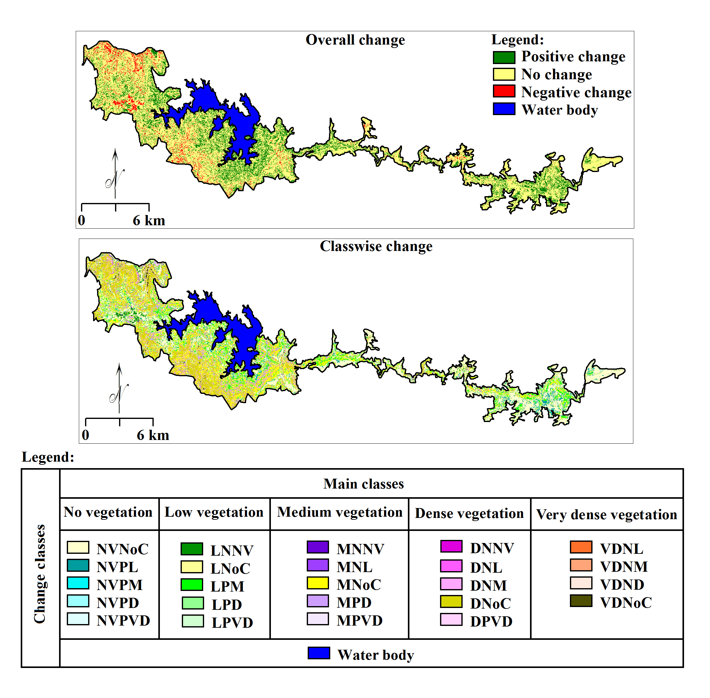
Classified raster images (Figure 13) for 2002 and 2009 were combined using cross operation in Ilwis for forest CD. 25 classes were created in this combination and similar classes merged to get meaningful categories (Table 4). Overall changes were estimated as ‘negative changes’, ‘positive changes’ and ‘no-changes’. Further, class wise changes also estimated to know the transformations from one class to another (Table 5) as ‘positive change, negative change and no-change.


 ,
Vijay Bhagat 1
,
Vijay Bhagat 1