Keywords

Watershed management , RUSLE , Remote Sensing , GIS , Soil

1 . INTRODUCTION

2 . MATERIALS AND METHODS

2.1 Study Area

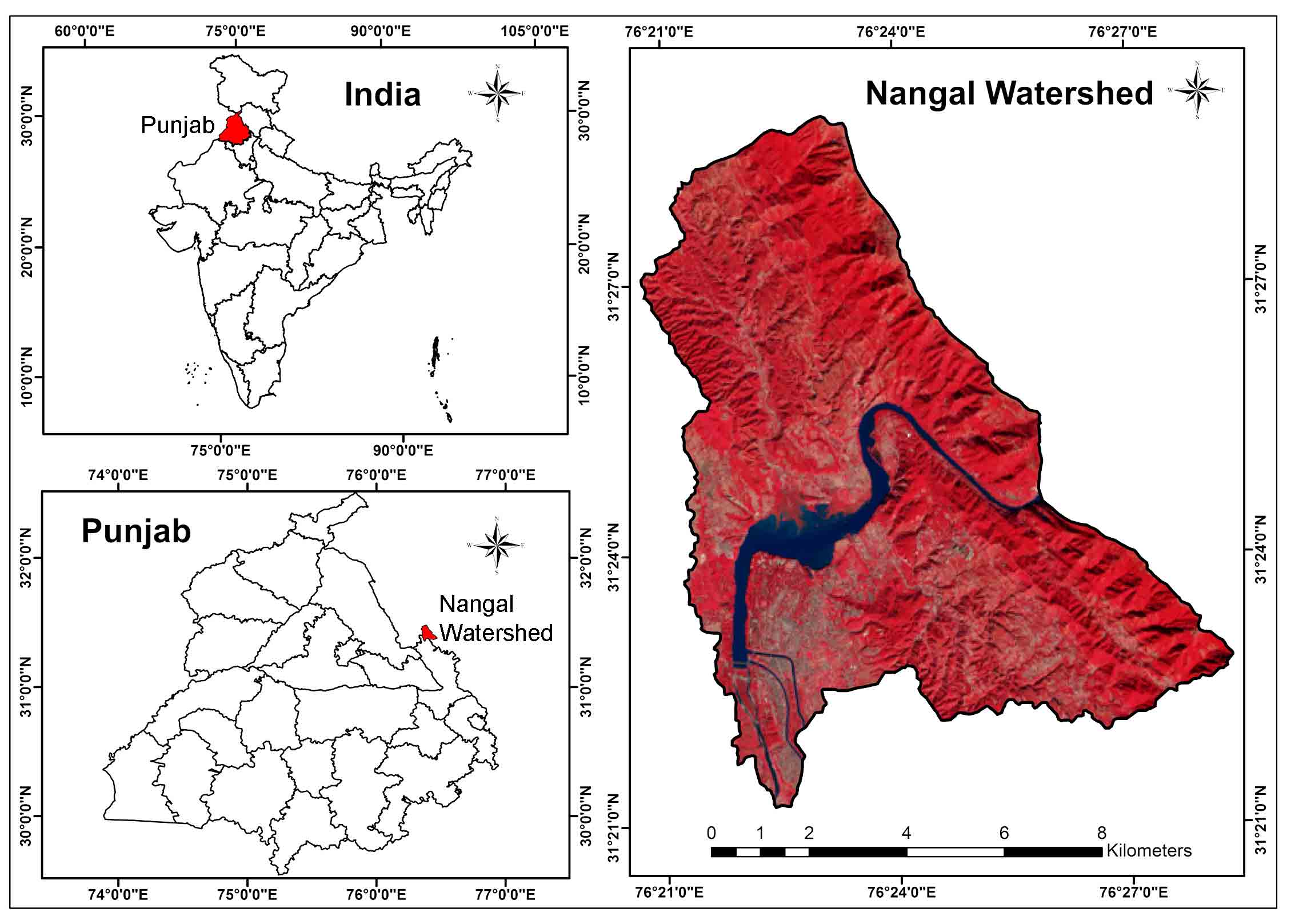
The present study was carried out over a macro- watershed upstream of Nangal reservoir with a total area of 8390 ha, selected mainly because of the spatial diversity of plant cover and the variety of soil classes and slope (Figure 1). The climatic characteristics indicate generally dry hot summer (except in the south-west monsoon season) and a bracing cold winter. The temperature ranges from minimum of 4°C in winter to 45°C in summer. The study area lies in the foothill regions of the Siwaliks where potential soil erosion rate is maximum. The point of interest in the study was to see whether RUSLE integrated in GIS environment was being able to be captured the soil erosion at this spatial scale and variation.

Figure 1. Study area: Nangal watershed of Punjab, India

2.2 Data Used

Three sets of Landsat-8 images (Kharif, Zaid and Rabi) were used in this work for generating thematic layers of land use / land cover (Table 1). ALOS PALSAR digital elevation model was used to derive elevation data. Rainfall data used for deriving R factor used in RUSLE was generated using Tropical Rainfall Mapping Mission (TRMM) datasets of last 18 years. Available soil map on 1:50000-scale was used for soil erodibility (K) extraction. Field survey was also conducted in three different seasons for validation of the final output by collecting GCPs.

2.3 Analysis and Visualization

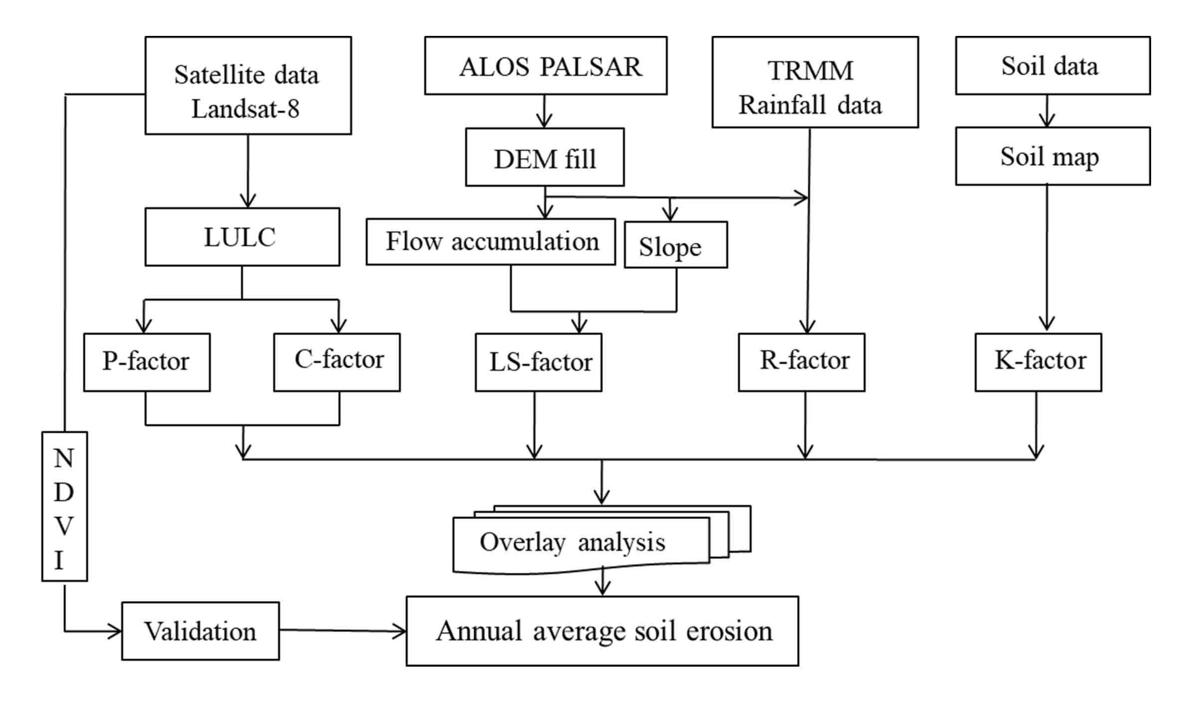
Implementation of the RUSLE model in GIS involves creating a work flow in computer based environment that includes input data processing, model computation, and analysis of results (Figure 2). The GIS provided powerful tools for analysis, visualization of modeling and specialized tools to perform model calibration and validation.

Figure 2. Methodology

2.4 RUSLE Model

RUSLE is often used to monitor soil erosion in agriculture watersheds ranging from macro to mini watersheds across the world (Udayakumara et al., 2010). This model was particularly selected for this study because of its demonstrated effectiveness. The RUSLE (Renard et al., 1997) model can be expressed as equation (1) and the methodology followed to map soil erosion.

\(A=R×K×LS×C×P\)

A = Computed soil loss per unit area per year (t/ha per year); R = Rainfall erosivity factor (MJ mm ha-1h-1year-1); K = Soil erodibility factor (t ha MJ-1mm-1); LS = Slope length and steepness factor (dimension less); C = Cover management factor (dimension less); P = Support practice factor (dimension less).

2.4.1 Rainfall Erosive Factor (R)

The rainfall erosivity factor is measured by rainfall intensity thus R basically explains the effect of raindrop on the ground. The modeling of R factor in GIS environment requires continuous satellite retrieved precipitation data. Therefore, monthly rainfall data product of TRMM satellite was downloaded over the study area for 18 years (1998-2015) and used to calculate the R-factor. Random 50 points were plotted over the study area. The locations and altitude of each point was calculated. Multiple regression models were used to derive a coefficient against each point’s altitude, longitude, latitude and rainfall. Finally rainfall intensity was calculated using the equation given by Van der .

\(R=a.p_j\)

\(p_j\)  is rainfall intensity in mm, a = coefficient derived from the multiple regression model.

Figure 3. Rainfall pattern (1998-2015)

Figure 4. Thematic maps: (a) Rainfall erosivity factor, (b) Soil erodibility factor, (c) Slope length and steepness factor and (d) Land cover management factor

2.4.2 Soil Erodibility Factor (K)

Soil erodibility is a function of soil texture, structure (e.g., macro porosity, aggregate properties), organic matter content, hydraulic properties and wetness of soil due to rain water and runoff (Blanco-Canqui and Lal, 2008). In this study available soil map was used to derive the soil erodibility (K) classes using standard classification scheme (Table 2). Since this watershed has thick forested layer whereas detailed field survey were not possible.

2.4.3 Slope Length and Steepness Factor

The topographical factors slope length (L) and the slope steepness (S) represents a ratio of soil loss below specified condition to any site (), it is a unit less factor.The highest and the lowest slope represent the maximum potentiality of soil erosion as LS factor generate high overland flow velocity and similarly higher runoff (Zhao et al., 2020). To obtain slope length (L) and slope steepness (S), ALOS PALSAR DEM data was used. This resolution was chosen by accurately defining flow direction in the watershed, using the “flow direction” tool of the Arc GIS software. Slope length corresponded to 10.0 m, when water flow was perpendicular to the pixel line and 14.14 m when it was diagonally oriented. The slope length factor was computed using the equation below:

\(L= (µ/22.1) m\)

Where, L  = Slope length factor, µ = horizontal projected slope length (m)

m = slope length exponent, (µ=flow accumulation X  cell size)

In this equation ‘m’ slope length varies based on slope steepness, m equals 0.5 if the slope is 4.5% or more; 0.4 if the slope is 3-4.5%; 0.3 if the slope is 1-3% and 0.2 of uniform gradient of less than 1% (Wischmeier and Smith, 1978).

2.4.4 Cover Management Factor (C)

The C-factor is important because it helps to indicate how soil loss potential will be distributed in time under different land use/land covers and during crop rotations, construction or other management activities (Thomas et al., 2018). To identify the C-factors, GIS techniques were used to extract thematic layer of land use / land cover of the study region from the satellite imagery. Then the literature based C-factor values were assigned for different land use / land cover in the study area according to Table 3.

2.4.5 Support Practice Factor (P)

Support practice factor represents the positive impacts of support practices on the soil it is often described as the ratio of soil loss by a support practice to that of straight-row farming up and down the slope (Figure 4e). The P-factor indicates conservation practices adopted in the watershed including terracing, bunding, strip cropping, check dam etc.The value of P- factor ranges from 0-1, in which 0 values represent high-quality preservation practice and the value resembling one indicates poor protection practices (Morgan et al., 1998). In catchment areas often several mitigation practices like terracing and contour tillage among other practices cannot be reflected in land use maps (Fu et al., 2005). Therefore, P-factor information was calculated through empirical method proposed by (Wener, 1972):

\(P = 0.2+0.03×S \) ,

Where, S  = Slope steepness, P  = P-factor

2.4.6 Annual Soil Loss (A)

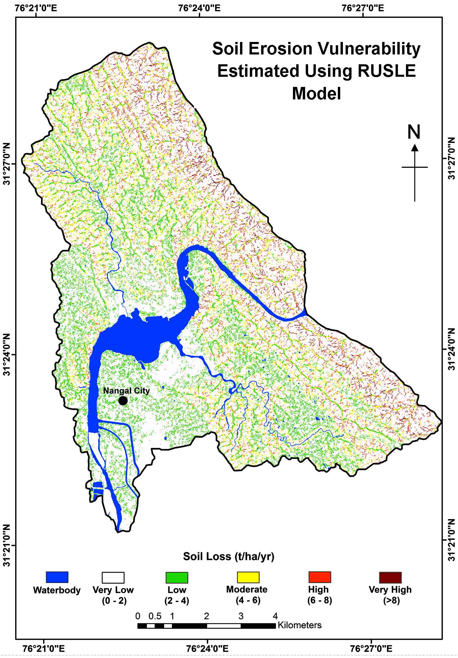
Soil loss determined using the RUSLE model using the Arc GIS software, was classified into five classes of soil loss: 0-2; 2-4; 4-6; 6-8 and >8 t/ha/yr.

Figure 4. Thematic maps: (e) Support practice factor and (f) Soil loss estimations

3 . RESULTS AND DISCUSSIONS

3.1 Rainfall Erosivity Factor (R)

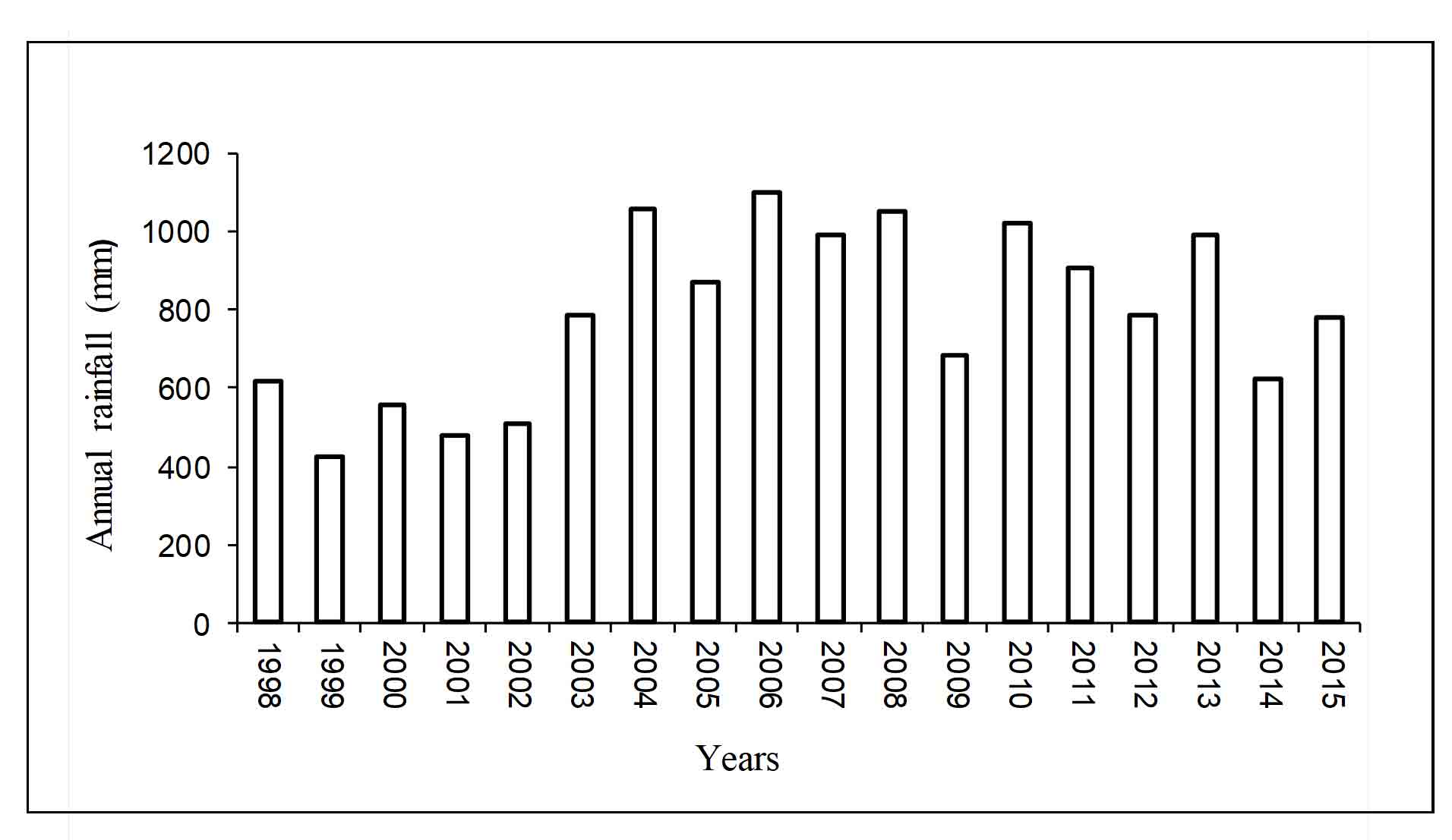
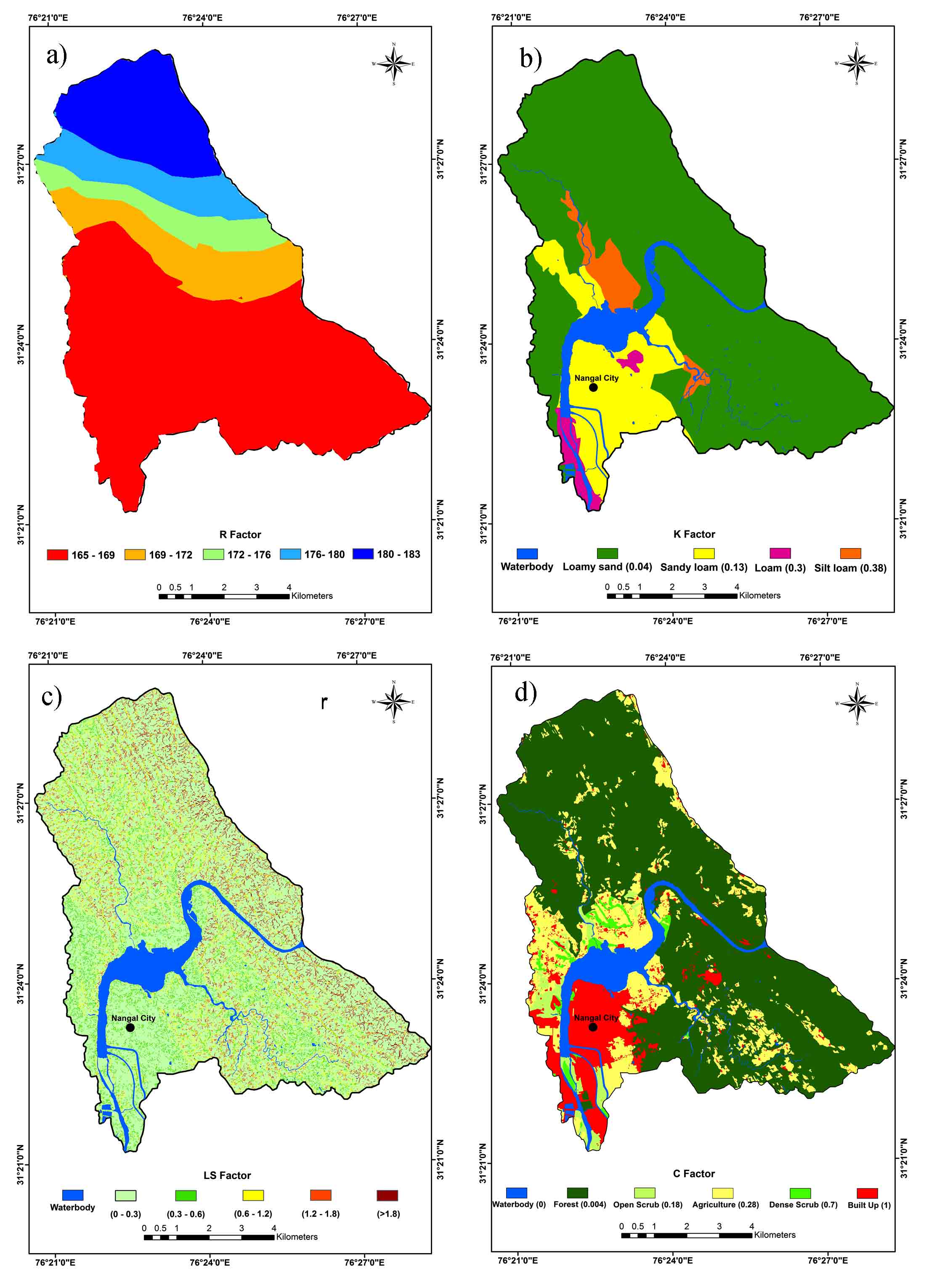
Since many studies often indicate that rainfall is the main indicator of soil erosion in any region therefore the pattern of rainfall in this region needs to be studied carefully. The monthly rainfall datasets were summed up to get the annual rainfall of each year over the study area. More than 400 mm of rainfall is witnessed in all the years and an average of 800 mm has been observed in this region over 18 years (Figure 3). In the present analysis average annual rainfall was used for R-factor calculation (Figure 4a).

The estimated R-factor ranges from 165 to 183 mm.ha^-1 hr^-1/year in the study area. The R-factor calculated has been divided into five major zones as seen in Table 4 and Figure 4(a). 165-169 mm.ha-¹hr^-1/year covers 5307 ha, 169-172 mm.ha^-1hr^-1/year covers 667 ha, 172-176 mm.ha^-1 hr^-1/year covers 563ha, 176-180 mm.ha^-1 hr^-1/year covers 526ha and 180-183 mm.ha^-1 hr^-1/year covers 1327 ha. This region experiences orographic type of rainfall, the foot hill region in the northern part of the study area experiences heavy rainfall and gradually the erosivity rate decreases as the land slopes down towards the plain.

3.2 Soil Erodibility Factor (K)

The study area is classified into four major soil erodibility classes based on soil texture. The study area comprises of four major soil textural classes i.e. loamy sand, sandy loam, silt and loam (Figure 4b). Maximum area is covered by loamy sand with an average soil erodibility factor of 0.3. The sandy loam soils possess an average erodibility factor of 0.13. Silty loam soils found in small patches provides an average of 0.38 soil erodibility factor. Very small patches of loam soils are found in the southern part of the study area. The silt loam soils K value as 0.38 occupies 328 ha of land, whereas sandy loam soils and occupies 1504 ha of land. Table 5 shows the distribution of the soil erodibility factor.

3.3 Slope Length and Steepness Factor (LS)

Topographic factor represents the basic influence of slope length and slope steepness on erosion process. LS- factor was calculated in ARCGIS by considering the flow accumulation and slope in percentage as the input factors. From the analysis, it is observed that the value of topographic factor increases as the flow accumulation and slope increases. The general slope of the region ranges between 0 and 1.8 from east to west. Maximum slope of the area is between 0 and 0.3 which occupies 6895 ha of land in the study area. Only 53 ha of land is under very high steepness factor influence which is in the hilly forested region bounded on the right hand part of the study area. Table 6 shows the distribution of slope length and steepness factor and Figure 4c demonstrates slope steepness factor.

3.4 Cover Management Factor (C)

Land use and land cover helps to understand land utilization pattern of any region and in turn land utilization helps to understand the erosion rate of that particular land cover. Thus, cover management is one of the crucial factors. The study region is mainly covered by dense forest, which is around 5448 ha in the eastern part and 0.004 is the C-factor in this region because the rainforest in this region contains huge tall trees with high density canopy cover which protects the ground below from random erosion factors (Figure 4d). Around 1301 ha land is covered by crop land which is vulnerable because this region goes under three cropping season thus soil particles are open to more erosion this region has a cover factor of around 0.28. Urbanization has contributed towards erosion to a great extent and it is most vulnerable land use because it spoils the top soil totally and covers an artificial concrete floor. Thus, 787 ha of land in the study area gave C-factor of 1. A very small part of the land is bare which are almost a waste lands it covers an area of 183 ha and has a C-factor of around 0.18 this land is affected only by natural geomorphic agents and not by any other external agents. Land without scrub has been given 0.7 C-factor because scrub does not have much of canopy cover to protect the soil. Water body in this region covers around 554 ha which is 0 C-factor because it is the least receptive land cover towards erosion. Table 7 shows crop management factor distribution.

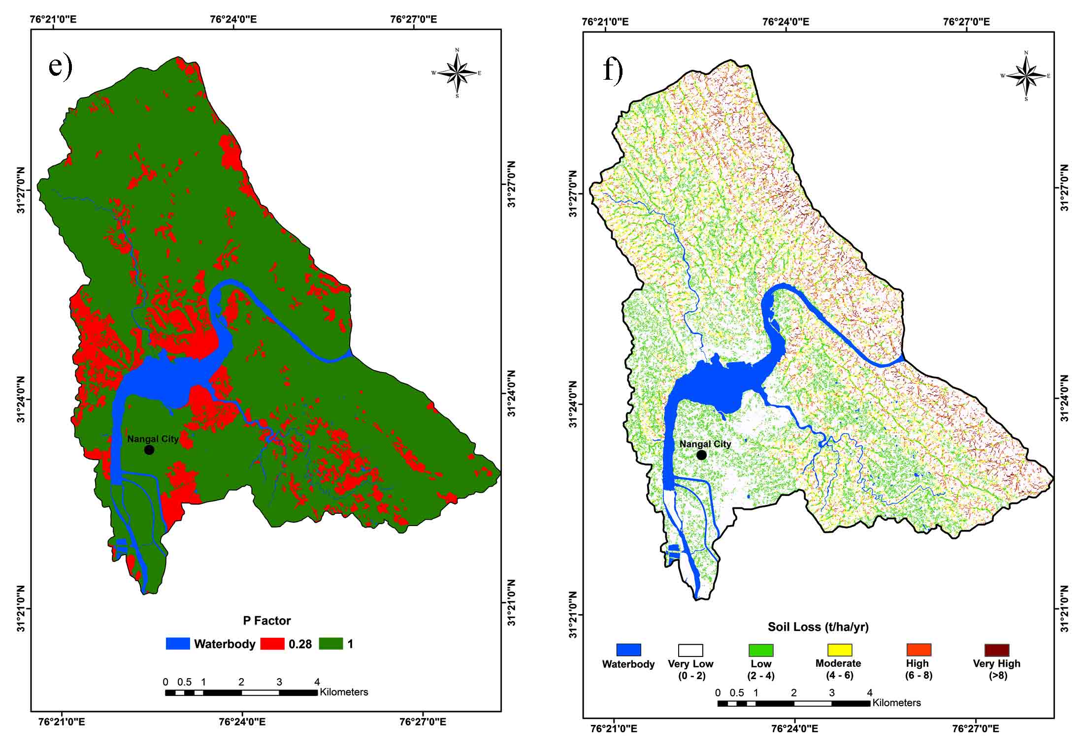
3.5 Support Practice Factor (P)

The analysis clearly shows that the area can be divided into two major classes according to support factor. The crop land in this region although is prone to more erosion due to exhaustive agriculture practices but these regions also go for green manuring at frequently after each crop rotation in three different seasons therefore, P- factor in this region is 0.28 (Figure 4e). However, rest of the land use and land covers like water body, dense forest, land without scrub, land with scrub and settlement does not have any managerial practices over this region therefore, 1 is distributed over these areas (Table 8).

3.6 Annual Soil Loss (A)

Integration of soil erosion parameters in RUSLE model in GIS environment provided annual soil loss at pixel by pixel basis to study the spatial distribution of soil erosion in the study area (Table 9, Figure 4f). The area can be graded into five vulnerability zone like very low, low, moderate, high and very high. 

It is seen that 7116 ha area is under erosion rate of 0-2 t^-1/ha^-1/yr, 663 ha area is under erosion rate of 2-4 t^-1/ha^-1/yr, 370 ha area is under erosion rate of 4-6 t^-1/ha^-1/yr, 370 ha area is under erosion rate of 6-8 t^-1/ha^-1/yr, 186 ha area is under erosion rate of 6-8 t^-1/ha^-1/yr and 55ha area is under erosion rate of 6-8 t^-1/ha^-1/yr. Immediate attention needs to be given to the 55 ha of land which is very highly prone to soil loss. Very high erosion rate is witnessed in the lower foothill parts of the hilly mountains because the river gushes down the slope and erodes the slopes by lateral and vertical movement of water downwards. Since Nangal Dam controls the water management factors in two major agricultural states of Punjab and Haryana, it can be affected adversely any time due to the high erodibilty in the upper reaches of the study area, thus management practices needs to be implemented properly to save the natural resource in the region.

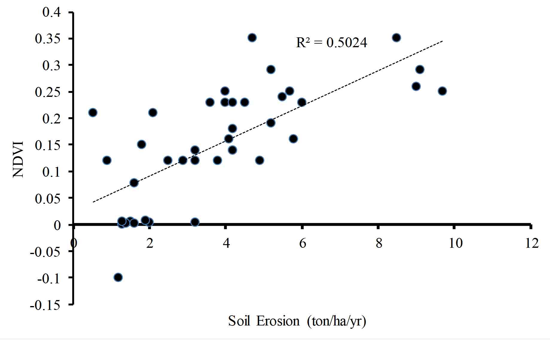
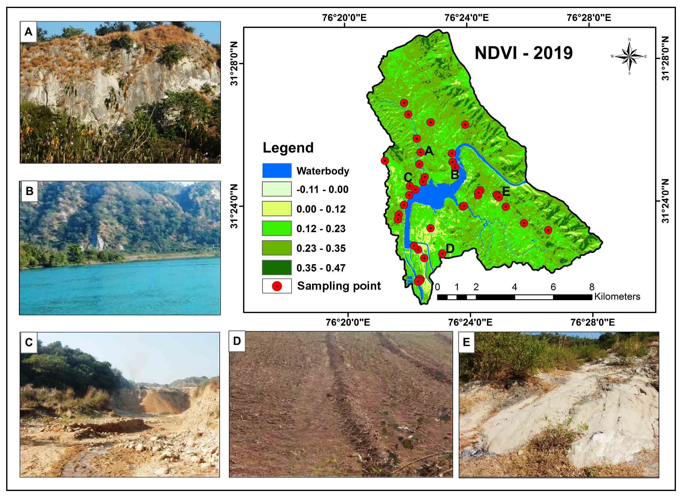
3.7 Validation of Results

Several workers reported integration of RUSLE in the GIS environment sans validation of soil loss estimation, which needs to be carried out to evaluate the authenticity of the results. The study area was very challenging as most of the places were inaccessible due to geographical hindrances and being upstream of the reservoir. Therefore, validation was done by collecting maximum points possible in the lower reaches on both sides of the river and few points in the lower foothills of the forested hilly areas. Random places were chosen and total of 35 points were visited, and ground information was gathered in correspondence to their latitude and longitude values using GPS. Further a Normalized Differential Vegetation Index (NDVI) map was generated in the GIS environment which included three seasons’ datasets to extract the vegetation cover percentage in the study area and a correlation of 0.5 was found between the NDVI and the soil loss erosion map t/ha/yr (Figure 5). This positive strong correlation suggests quite good accuracy level of the soil loss estimation map generated in the GIS environment (Figure 6).

Figure 5. Correlation between vegetation cover and soil losses

Figure 6. Distribution of ground truth points with photographs

4 . CONCLUSIONS

RUSLE can be easily integrated in the GIS platform and the inputs required for this model can be derived from multi-sources like satellite based data, available maps and in-situ observations. The topographic parameters can be readily extracted from DEMs facilitating GIS based erosion modeling. In spite of advances in sensor technologies, uncertainty and coarseness of critical parameters like spatial distribution of soils, and rainfall still remain the weak components of erosion modeling using RUSLE. The model results reasonably match with the observed field survey and majority of the area falls under moderate to low risk of soil erosion. Only, 55 ha of land is under threats of very high erosion rate per year. The results obtained from the study can assist in developing management scenarios and provide options to policy makers for managing soil erosion hazards in the most efficient manner for sustainable management plans.

Tables

Figures

Conflict of Interest

Acknowledgements

Abbreviations

References