The study focused on examination of spatial changes in urban areas using geospatial technology.
Markov Chain and CA-Markov techniques were used to model the LULC changes in the Adama district.
The model was verified by the Kappa statistics and also by the application of other validation techniques.
The growth of built-up areas in the last 37 years has risen from 2% in 1973, 10% in 2000 and 23% in 2010.
The identified changes in urban patterns will be useful for successful land use regulations and planning.
Abstract
In the last decades, Adama city has experienced drastic changes in its shape, not just in its vast geographical expansion, but also by internal transformations. Subsequently, understanding and evaluating the spatiotemporal variability of urban land use and land cover (LULC) shifts, and it is important to bring forth the right strategies and processes to track population development in decision-making. The goal of this analysis was therefore to examine LULC changes that have taken place over 37 years, forecast the long-term urban development in Adama City using geospatial techniques. To attain this, satellite data of Landsat 1973, 2000 and 2010 was downloaded from USGS Earth Explorer and processed using Arc GIS 10.5, Erdas 9.2, and Idrisi 32. A supervised classification technique has been used to prepare the base maps with six land cover classes that are accustomed to generate LULC maps. The maps are cross-tabulated to measure LULC changes, to look at land-use transfers between the land cover classes, to spot increases and declines in built-up areas in comparison to other land cover classes, and to determine the spatial changes in built-up areas. Finally, Markov Chain and CA-Markov techniques were used to model the LULC changes in the Adama district and to forecast possible changes in urban land use. The model was verified by the Kappa statistics and also by the application of other validation techniques. The growth of built-up areas in the last 37 years has risen from 2% in 1973, 10% in 2000 and 23% in 2010 and estimated about 60% over the next 30 years (2040).
The urbanization is playing a vital role in global development. Increased population and land requirement for settlement, economic and industrial growth, as well as its environmental effects, have also posed concerns in many countries. The world has great exceeding in city development in accordance to the United Nations (UN, 2000) and the Population Comparison Bureau (PRB, 2000). In 20th century, population in metropolitan cities was very quickly expanded from 0.22 billion to 2.8 billion. An enormous rate of urban development in the developing world will occur within the next few decades (Mesfin, 2009). In Asia and Africa countries, population becomes double in single century. Through 2030, cities and towns in the developing world will make up 81% of the urban population (Mesfin, 2009). The population growth rate in Africa was the highest in the world and it was 4.4% per year (Antonio, 2000). Ethiopia is still largely under-urbanized, taking into account the norms of Africa (Haregeweynet et al., 2012).
In the middle of 1930s, the urbanization rate will be faster (Antonio, 2000). Urbanization was increased between 1950 and 1965 with an average growth rate between 5.4 and 5.6 % per year indicate a doubling of the population in just 13 years. Urban population increase in the last 15 years has again been more than 5% and a high in the five-year period of 1985 and 1990, when the average rate of change was 5.93% (Mesev, 2008). Mostly, the rapid growth of the urban population is due to the difference between rural and urban development and significant rural-to-urban migration up to 1975, while the land reform program of 1975 created incentives and opportunities for peasants and other potential migrants to live in rural areas (Antonio, 2000).
Urbanization has been a product of industrialization in the countries of Europe and North America and has been linked to economic progress, while urbanization has arisen in the developing countries of Asia, Africa and Latin America as a result of population growth and large rural-to-urban relocations (Mesfin, 2009). According to Haregeweyn et al. (2012), many fields have been transformed from rural to urban. According to the 2007 census, Ethiopia has the second largest population in Africa with a total population of over 80 million. It has an annual growth rate of 2.3% and an overall annual population growth rate of 4.6% (Haregeweyn et al., 2012). According to Zubair (2006), the rapid rise of urbanization, the economic gains and the unplanned growth of cities have been resulted many negative effects. The majority of cities are horizontally spreading along the rail and road networks. Such enthusiasm of urban land cover may be caused by social, economic or industrial influences. There are already significant environmental issues that need to be closely examined and tracked for successful land use regulation and planning. In addition, fast population development and improvements related to urban land have attracted many scholars to study and track developments (Mesfin, 2009).
The unexpected urban development is now a major challenge, especially in developing countries where there is a shortage of consistent and accurate data, including spatial data. According to Mesfin (2009), the study of drastic shifts in LULC at continental, national and local level, and additional exploring the scale of potential changes, the existing geospatial expertise on land use dynamics and innovations already plays an important role. Remote Sensing (RS) and Geographic Information System (GIS) are now providing new tools for sophisticated landscape management. The remote sensing analysis allows patterning, system activity, adjustment at regional and local. This data provide a significant connection between localized ecological studies and intensive and international, state and regional conservation (Zubair, 2006). The urbanization, as a deep and also ongoing worldwide occurrence that has been going on for hundreds of years, has been researched by several scientists, concentrating on city growth, city sprawl, and the complexities and trends of urbanization (Antrop and van Eetvelde, 2000) noted that urbanization involves diverse and complex, changes to the rural environment in the, area of towns and cities, leading to very heterogeneous ecosystems. Gerten et al. (2019) have established the trajectory of urbanization expected to remain steady in the future, and will influence trends of land use in several respects. In addition, Keil (2018) claimed that the Earth is the ‘suburban planet’ and predicted that people will want to ‘make the world urban from the outside in’. The European, Environmental Agency (EEA, 2018) cautioned that urbanization, is unsustainable, contributes to soil waste, divides the landscape, and limits the ability of habitats to offer essential ecological services. Henderson and Turner (2020) shows that Europe, Latin and North America and the Caribbean as well as Western Asia tended to be entirely urbanized. Yang et al. (2018) reported that Chinese scientists have observed and marked uneven urban developments in various locations in the world, particularly in Benjin. In comparison, there is a limited research on urban development and its impacts using geospatial data. In order to evaluate land cover change and growth in Adama Region, a change, detection study was undertaken to evaluate the magnitude and scale of land-use change and estimation over time and space. The findings measure LULC change patterns of change in the city and show available satellite data to provide, reliable, cost-effective means of measuring and assessing the land cover changes through a spatial-temporal context that can, be used as guides to land form management, and policy decisions on various themes relevant to land cover, such as agricultural areas, croplands, forest lands.
2 . METHODOLOGY
2.1 Study Area
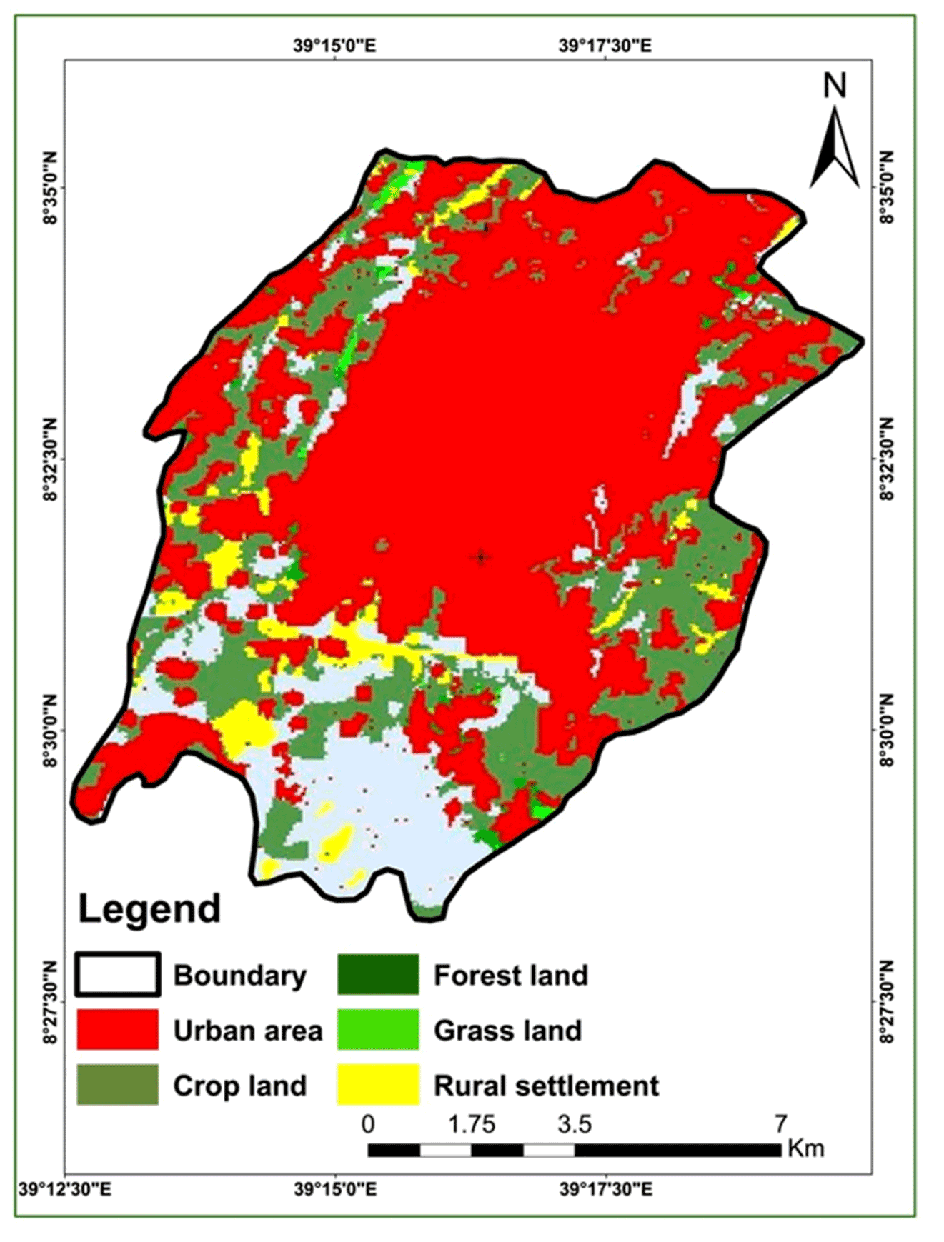
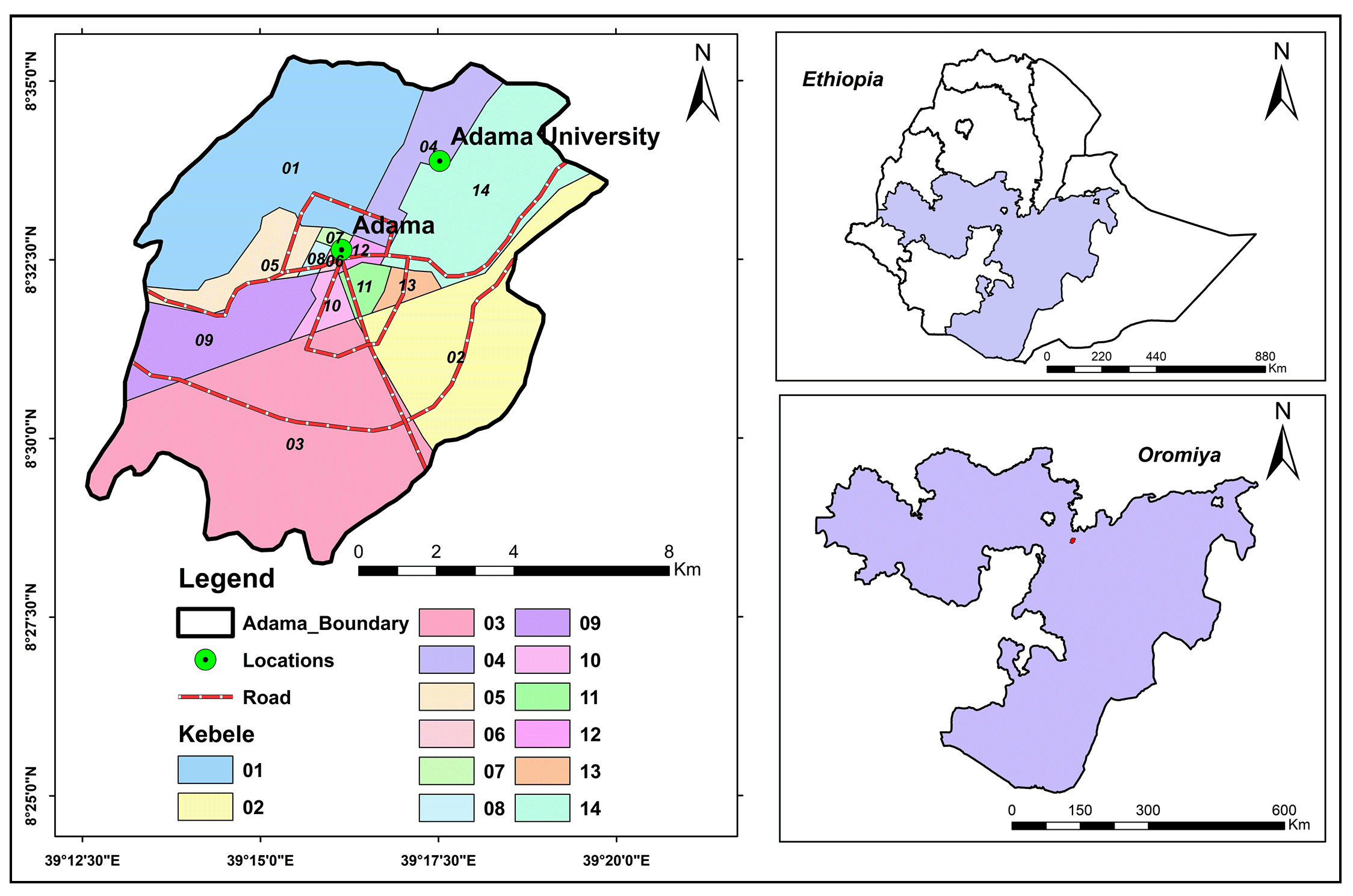
Adama city is located 100 km from southeast of Addis Ababa about 8º 35' 00" and 8º 36' 00" N and 39º 11' 57" to 39º 21' 15" E (Figure 1) at an average altitude of 1620m above the sea level. Adama is situated in the Eastern Shewa region which is part of the central plateau. According to the 2007 census, the total population of Adama city was 222023. Besides, the population growth rate of the city (5.4% per annum) was estimated to be higher than the national average (2.5% per annum) (CSA, 2007). CSA’s 1994 Population and Housing Census and 1999 National Labour Force Survey (NLFS) indicates that there were about 187,000 people living in Adama City in 2004. Nevertheless, the year 2002-2003 estimates of the City Administration reveals that the City population is known to be well over 200000. The proportion of male to female during the period was about 48.5 to 51.5 percent revealing further that the sex ratio was 94.0 percent, which implies little excess of women over the men (about 100 females for each 94 males). Furthermore, according to the CSA’s 1994 census, about 33.6 percent of Adama residents were below the age of 15. Similarly, the data further reveals that populations within the working age group (15-64) and above 64 years of age were 63.5 and 2.9 percent, respectively.
Figure 1. Location map: Study area
As a result, various studies [CSA, 1984, 1994, 1999 and Adama Project Office’s (APO) socio-economic surveys, 2004], Adama has been one of the areas both in the region and the country that receives heavy influx of migrants each year. For instance, the 1984 Census indicates that 53.7% of the City populations were migrants. Similarly, after a decade, in 1994 the second census showed that the extent of migrants were 53.6%. The finding of the 1999 NLFS neither contradicts with the above mentioned two census outcomes. According to the results of the NLFS, hence, 52.1% of the populations of Adama City were contributed from migrants in 1999. The findings of many socio-economic surveys undertaken by APO in 2003-2004 too, confirm that immigration stand out as one of the major issues in Adama City. In the Poverty and Socioeconomic Problem survey undertaken in Adama, about 68.0% of the poor households were migrants. Similarly, in the same study it was found that about 83.0 percent and 87.0 percent of the commercial sex workers and street occupants were migrants, respectively (APO, 2004). The census data further points that Adama households were estimated to have about 4.8 persons on the average. Thus, it could be possible to estimate that about 39.0 thousand households were residing in the city in July 2004.
2.2 Data and Processing
In this research, geospatial technology was, used to detect the urban changes in a particular timeframe and, to examine patterns and trends of transition. Satellite imageries are almost ideal to provide details on the numerous geospatial patterns on the surface of the earth. However, attention must be, given to the degree of, resolution, the degree of accuracy of the image, through processing. However, similar to Mas (1999), it was suggested that it would be impossible to collect multi-date data at the same time of year. According to Gluch (2002), satellite image, MSS, ETM+ and, ETM+ satellite data, are typically used, for their multispectral and environmental, significance (Table 1). The pre-processing and post-image processing analysis was carried out to increase the images accuracy, and the readability of the applications using GIS and ERDASS software. The spheroid and the date are referred to in WGS84. All images were, geometrically, co-registered using ground control, points in the UTM projection. Ground Control Points (GCPs) obtained from identified ground points, the coordinates of which can be precisely placed on digital, imagery.
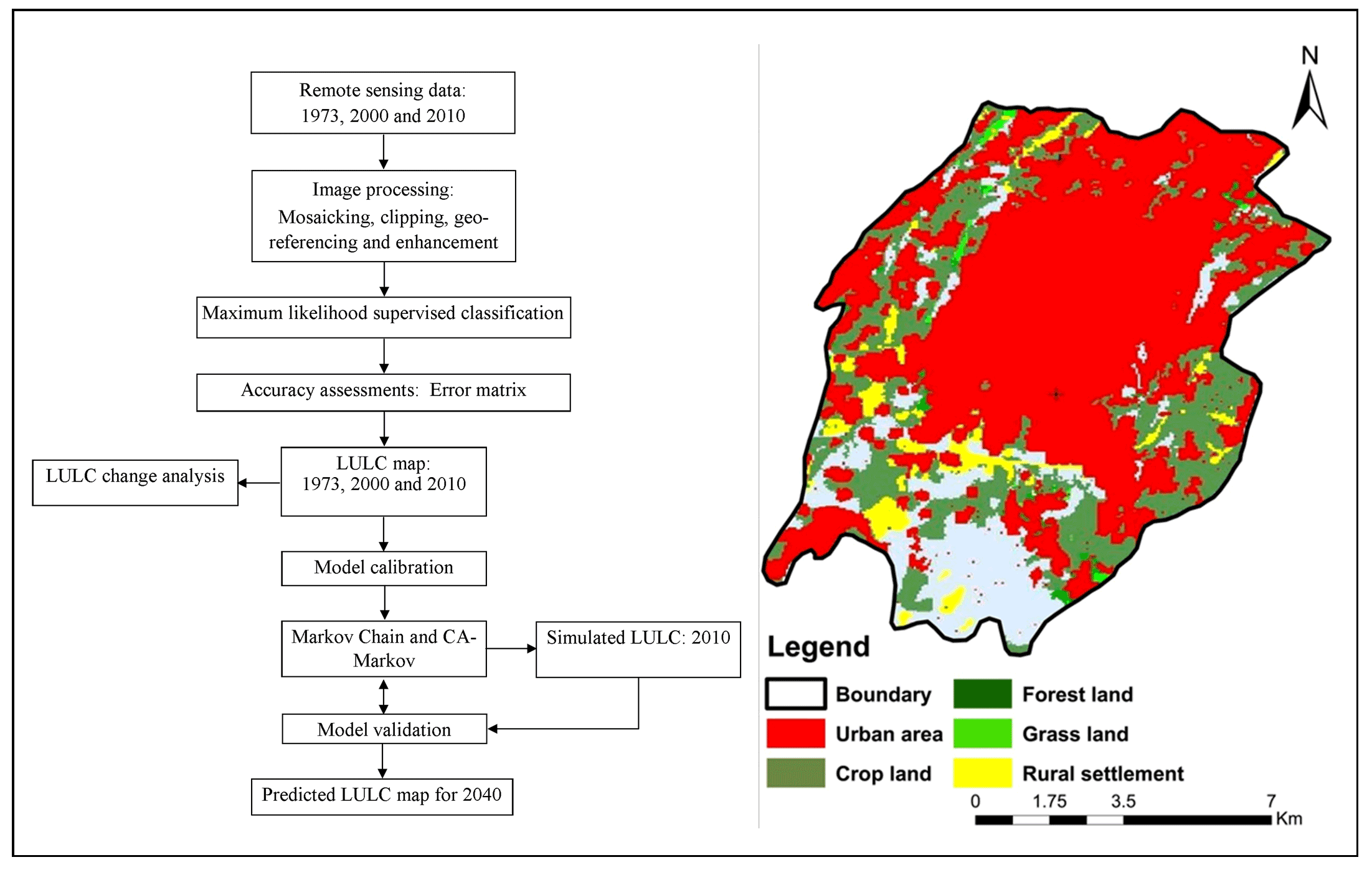
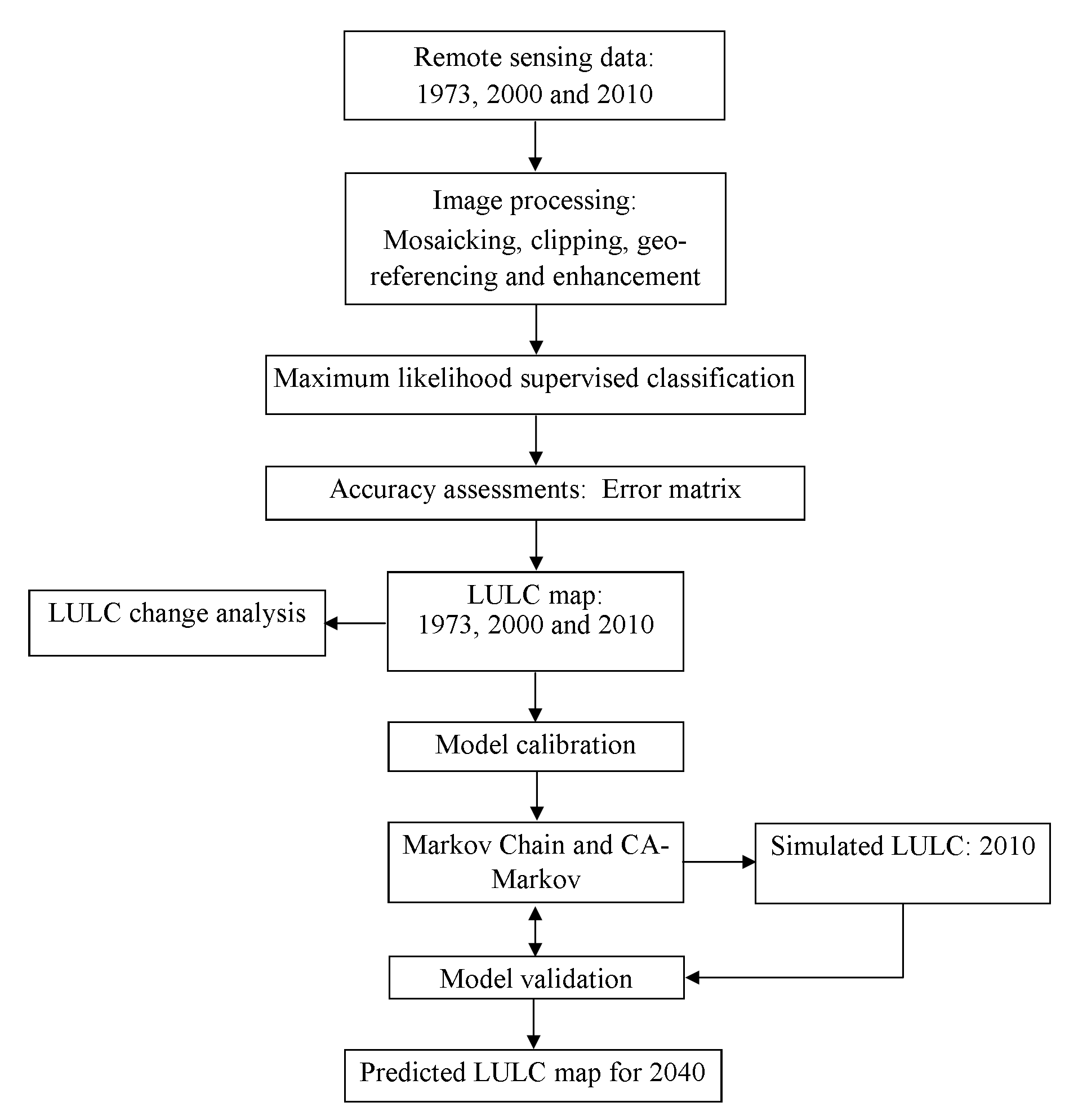
Figure 2. Methodology
Table 1. Sensor, spatial resolution and acquisition
Sensor
Spatial Resolution
Acquisition time
Producer
MSS
57m
January 1973
EMA
ETM
30m
January 2000
EMA
ETM
30m
January 2010
EMA
Ground Controls Points (GCPs) were collected by using Global Positioning System (GPS). Hence, Arc Map 10.5, ERDAS Imagine 2014, and IDRISI 32 software tools were used to make land-use modeling and future prediction. Besides, IBM SPSS statistics 20 and Microsoft Excel for tabulating and graphical representation were used.
2.3 Land Cover Nomenclatures
In order to make sample collection and classification easy, land cover nomenclatures are required to create and define the possible LULC classes first. Although the focus of the paper is on built-up areas, LULC map of the study areas was first generated using land cover classes presented in table 2. The LULC classes applied in this study were adopted from the classification used by European Environment Agency (EEA), Coordination of Information on the Environment (CORINE), which describes LULC (and partly land use) according to a nomenclature of 44 classes organized hierarchically in different levels. Moreover, due to the geographical location of the study area in Tropics, the CORINE land classes adopted was not entirely applied. It is a land cover class which is more applicable for Temperate and cold Polar Regions. In order to solve this challenge,
Table 2. Nomenclature of LULC classes
Land classes
LULC
Description
C1
Forest land
Natural and manmade forests, sparsely planted trees wood land shrubs.
C2
Grass land
Grass, shrubs, bushes.
C3
Bare land
Open fields with, little to without trees, beaches,,dunes, grass, sparsely vegetated areas and bare gravel.
C4
Crop land
Permanent crops.
C5
Rural settlements
Permanent residential discontinuous and constant urban fabric.
C6
Urban and associated areas
Residential, commercial units and industries, road and, other related property.
AFRICOVER land cover classification system which is widely applied at East African Countries (Africover, 2002) was integrated. For the sake of simplicity, the researcher modified the descriptions of some of the land cover classes considering the land cover diversity of the study area. Six major land cover nomenclatures (forest land, grass land, bare land, crop land, rural settlement and urban areas) were used to produce the final LULC map of the study area.
2.4 Image Classification
It is known as the extraction from raw remotely sensed digital satellite data of distinct groups or themes, LULC categories. It is also a technique used to classify various features such as city land cover, plant forms, anthropogenic systems, mineral resources or improvements in all of, these characteristics of the satellite image. In order to increase the accuracy, of classification, it is important to choose the right classification process. This will also allow the analyst to successfully identify the land changes (Elnazir et al., 2004). The supervised classification technique was used in this analysis. Manual detection of the point of interest, the areas as a reference within the photographs is needed to conclude the spectral signature of the identifying features. This is one of the most common types of classification strategies in which all pixels with identical spectral values are automatically classified into ground cover groups. Classification and post-classification overlays and thematic land-cover change maps for the years 1973, 2000 and 2010 were developed by using supervised classifications for the study area. Six major LULC classes: rural settlement, urban and associated areas, bare land, crop land, grass land and forest land areas were performed to detect potential details for mapping the patterns and extents of LULC change as well as to find out the magnitude of changes between the years of interest years 1973, 2000, 2010 and predicted map of 2040.
3 . CLASSIFICATION, RESULTS AND VALIDATION
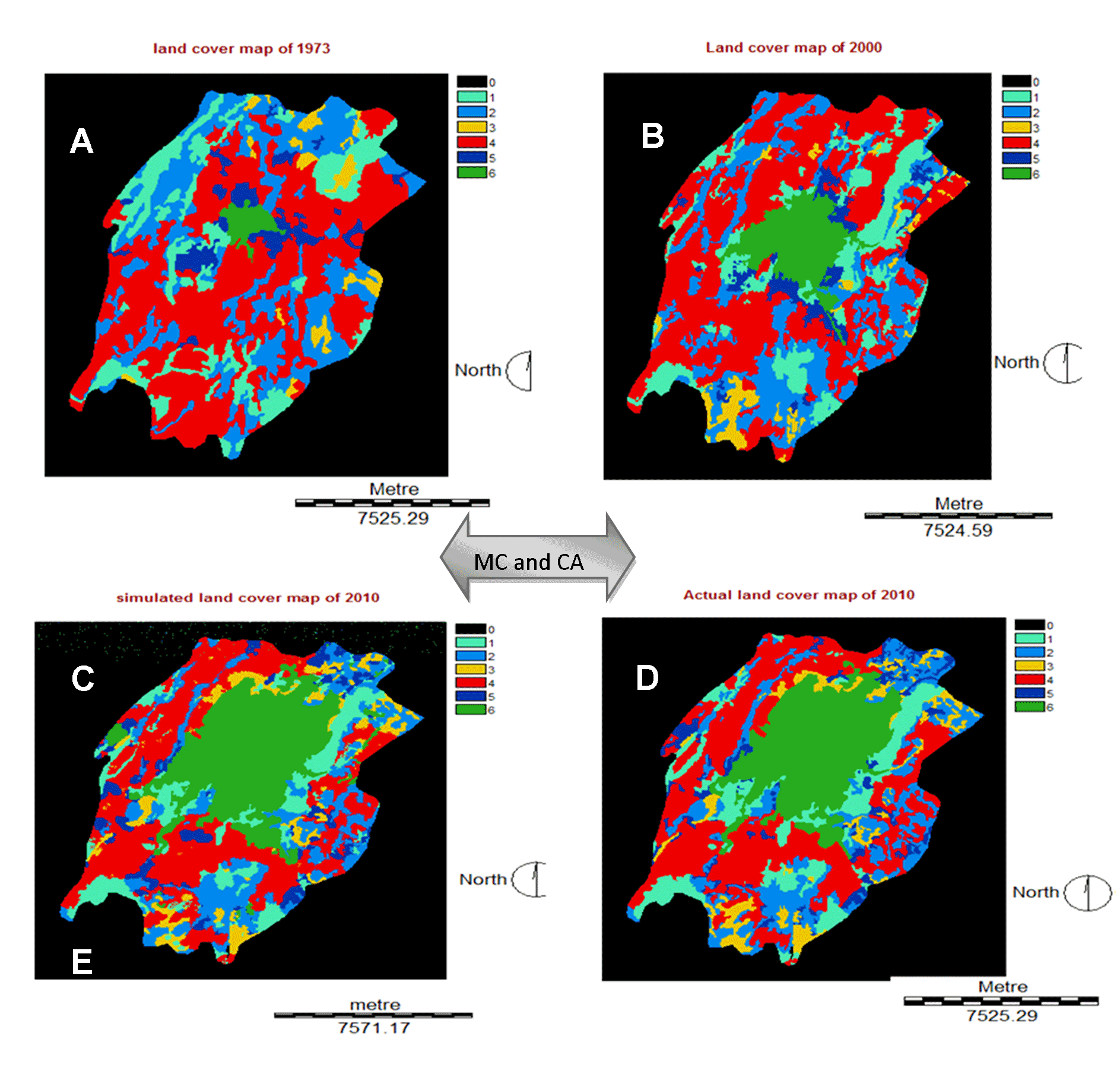
After a supervised classification has been carried out, the land cover maps as well as post-classification algorithms are performed as given in figure 3 to 5 and table 4 to 6. The accuracy of a categorized map must be measured and compared to the referenced data using an error matrix. The accuracy measurement in this analysis was rendered using the original mosaic image for the years 1973, 2000 and 2010.
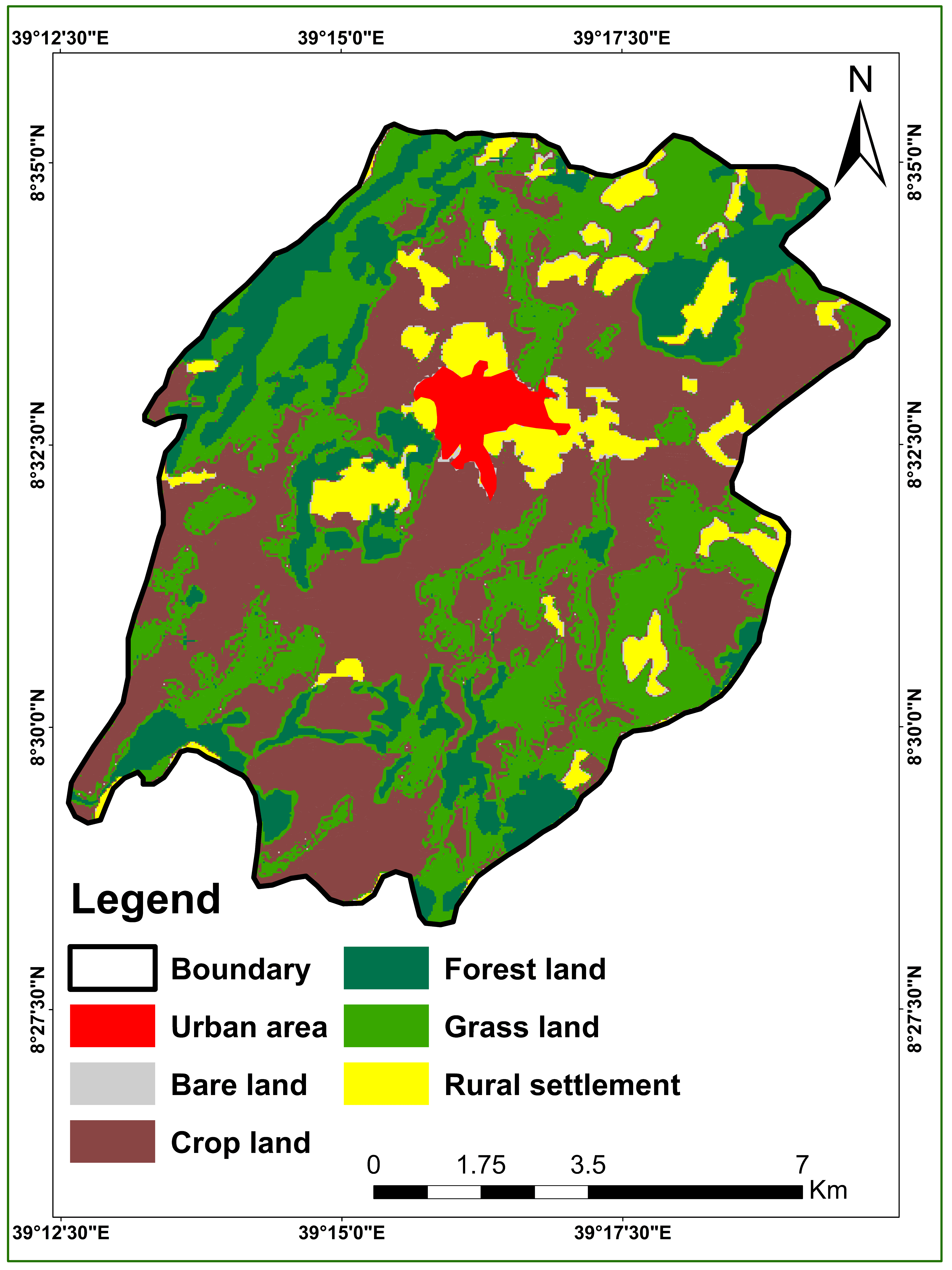
Figure 3. LULC: 1973
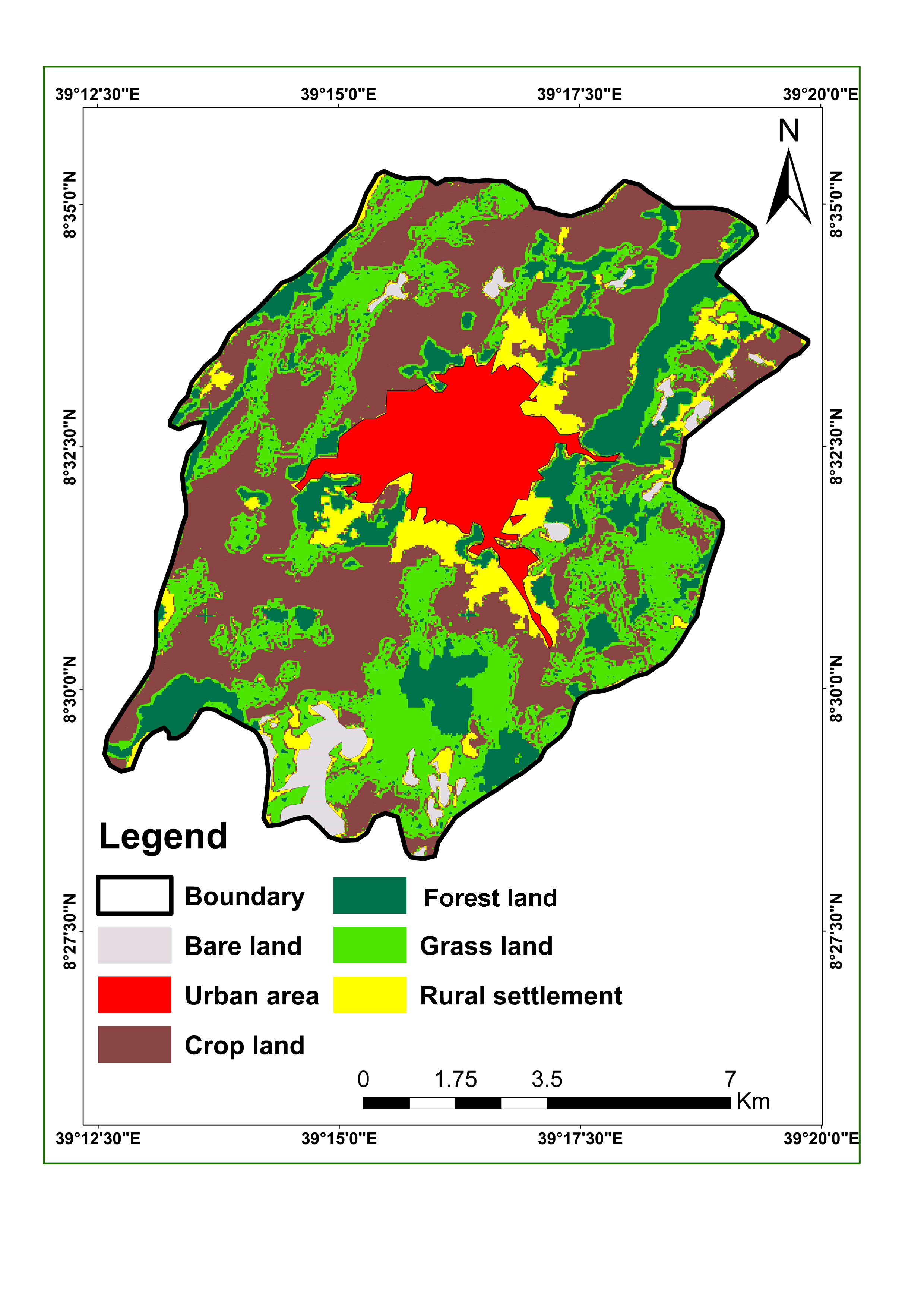
Figure 4. LULC: 2000
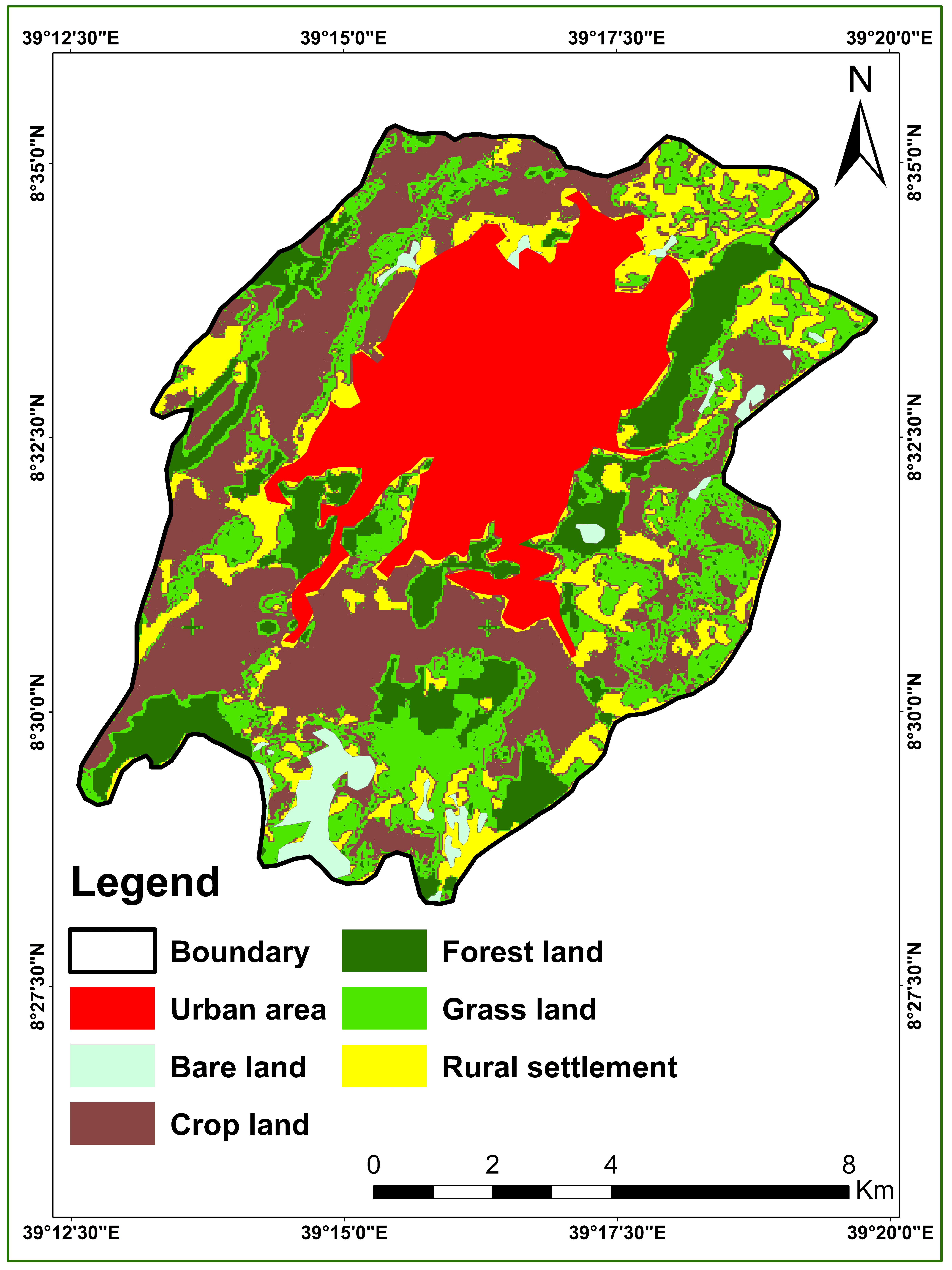
Figure 5. LULC: 2010
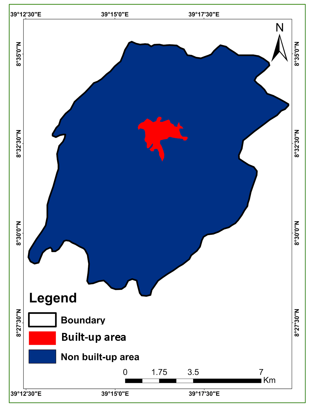
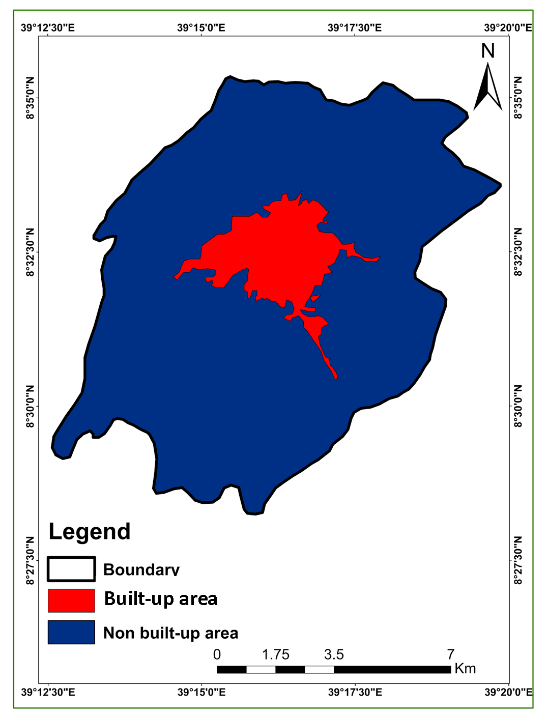
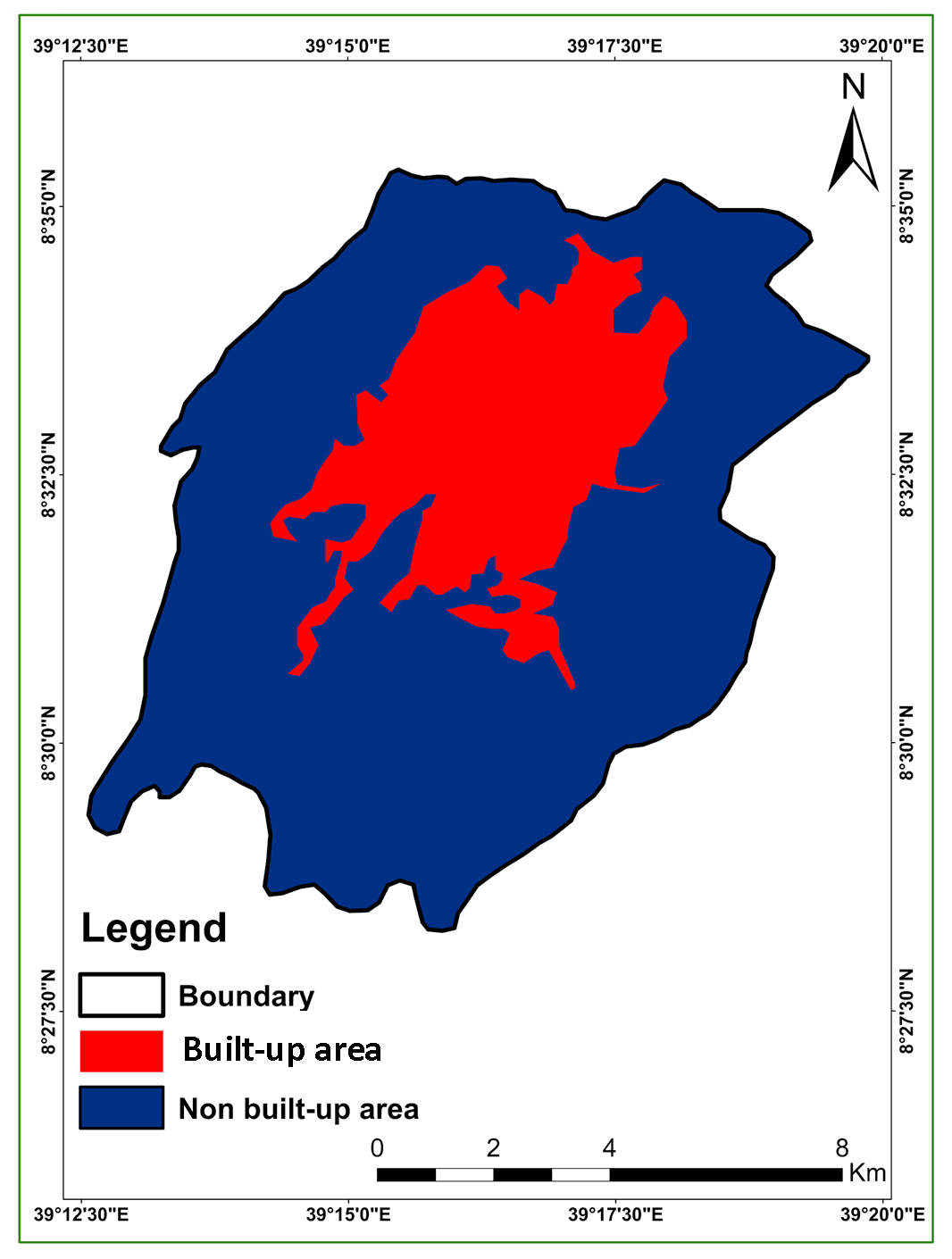
Figure 6. (a) Built-up and non-built-up areas: 1973
Figure 6. (b) Built-up and non-built-up areas: 2000
Figure 6. (c) Built-up and non-built-up areas: 2010
Table 3. Surface characteristics occur in various composite images
Features
True Color
RGB321
False Color
RGB432
SWIR (GeoCover)
RGB742
Trees and bushes
Olive green red
Olive green red
Shades of green
Crops
Medium to light green
Pink to red
Shades of green
Wetland vegetation
Dark green to black
Dark red
Shades of green
Water
Shades of blue and green
Shades of blue
Black to dark blue
Urban areas
White to light blue
Blue to gray
Lavender
Bare soil
White to light gray
Blue to gray
Magenta, lavender or pale pink
Clouds
White
White
White-pink-lavender
Snow/ice
White
Light green-blue
Medium blue
Table, 4. Confusion, matrix for LULC map:1973
Classified map
LULC
Reference map
Forest land
Grass land
Bare land
Crop land
Rural
settlement
Urban area
Total
User’s accuracy
Forest land
24
1
0
0
0
0
25
96%
Grass land
5
13
0
0
1
0
19
68.42%
Bare land
0
0
27
0
1
0
28
96.4%
Crop land
0
0
3
62
1
8
74
83.78%
Rural
Settlements
0
0
0
2
14
0
16
87.5%
Urban areas
0
0
0
3
0
45
48
93.75%
Total
29
14
30
67
17
53
210
Producer’s
accuracy
82.2%
92.8%
90%
93%
82.35%
84.9%
Overall accuracy: 88.09%
Table 5. Confusion, matrix for LULC map: 2000
Classified map
LULC
Reference map
Forest land
Grass land
Bare land
Crop land
Rural settlements
Urban area
Total
User’s accuracy
Forest land
26
3
0
0
0
0
29
89.6%
Grass land
1
13
0
0
0
0
14
92.8%
Bare land
0
0
27
3
0
0
30
90%
Crop land
0
0
0
63
0
4
67
94.2%
Rural settlements
Urban area
Total
Producer’s
accuracy
0
1
2
1
13
0
17
76.47%
0
0
0
7
0
46
53
86.79%
27
17
29
74
13
50
210
96.2%
76.4%
93.1
85.1%
100%
92%
Overall accuracy: 89.52%
Table 6. Confusion, matrix for LULC map:2010
Classified map
LULC
Referenced Map
Forest land
Grassland
Bare land
Cropland
Rural settlement
Urban area
Total
User’s accuracy
Forest land
27
2
0
0
0
0
29
93.1%
Grass land
1
12
1
0
0
0
14
85.7%
Bare land
0
0
26
4
0
0
30
86.67%
Crop land
0
0
0
64
0
3
67
95.5%
Rural settlements
0
1
2
0
14
0
17
82.35%
Urban land
0
0
0
5
0
48
53
90.5%
Total
28
96.45%
15
80%
29
89.6%
73
87.67%
14
100%
51
94.1%
210
Producer’s accuracy
Overall accuracy: 90.95%
3.1 User’s Accuracy
The findings of user’s accuracy show that in 1973, the highest class accuracy (96%) for forest land and bare land and the minimum accuracy was estimated for grass lands (68.42%) (Table 4). Class precision ranged from 76.47% to 94.2% in 2000, although it ranged from 82.35% to 95.5% in 2010. The lowest, values of class accuracy were reported due to spectral similarity with other classes. As seen in table 4, 5 and 6, the lowest value was observed for grass land during the time of 1973 (68%) and the rural settlements for the years 2000 and 2010 with 76.47% and 82.35%, respectively. In addition, the resolution of Landsat data may have an impact on the classification of the image.
3.2 Producer’s Accuracy
The precision relates to the producers is number of pixels properly identified in each class divided by the total number of pixels of the class (total column). The highest values were for crop land, 93% (Table 4) and for rural settlement, 100% (Table 5 and 6).
3.3 Overall Accuracy
As shown in table 4, 5 and 6, the overall accuracies were 88.09% in 1973, 89.52% in 2001, and 90.95 % in 2010, respectively. Anderson et al. (1976) stated that the determined minimum average accuracy should be 85% for a consistent ground cover classification. However, Foody (2002) has demonstrated that it is not appropriate in the sense of a global norm for actual applications. In addition, Lu et al. (2004) claimed that the accuracy of change detection depends on the availability and consistency of ground truth data, the sophistication of the research region, landscape, the detection strategies used as well as classification and change detection schemes.
3.4 LULC Changes and Statistical Analysis
For the three study periods, the images are quantified and the results are presented in Table 7. From this table, urban areas have been increased with values of 2%, 9.6%, and 23% in 1973, 2000 and 2010, respectively.
Bare land has been increased between study periods (Table 7). It increases 3.4% in 1973 to 3.8 % in 2000 to 6.7% in 2010 and rural settlement 5.3% in 1973 to 5.2 % in 2000 (decreased), 5.2% in 2000 to 6% in 2010. The cropland decreases by 3% from 1973 to 2000 and 9.8% from 2000 to 2010. Forest land and grass lands were decreased in the study periods. Forest lands decreased from 16.1% (1973) to 15.3 % (2000) and by 12.8% in 2010; grass land decreased from 26.8% to 22.7%, and to17.9% in the same period.
Table 7. LULC in Adama city
LULC
1973
2000
2010
ha
%
ha
%
ha
%
Forest land
2188.9
16.05
2086.6
15.3
1747.9
12.81
Grass land
3658.1
26.83
3091.44
22.67
2438.9
17.89
Bare land
465.24
3.41
521.2
3.82
916.84
6.72
Crop land
6332.3
46.44
5917.9
43.4
4575.5
33.56
Rural settlements
718.9
5.27
710.2
5.21
816.3
6
Urban area
271.8
2.00
1307.9
9.6
3139.8
23.02
Total
13635.24
100
13635.24
100
13635.24
100
3.5 LULC Changes: Built-up Areas
In table 8, the percentage of built-up areas in 1973 was 2% and 10% in 2000 which was 8% more than last records. It was 23% in 2010. The figure 6 a, b and c illustrated that there had been a rapid shift in land use from unconstructed areas to built-up area. During this study period, crop lands were the most diverse group that led to the rise in built-up areas.
Table 8. Built-up and non-built-up areas: 1973-2010
LULC
1973
2000
2010
ha
%
ha
%
ha
%
Built up area
271.84
2%
1307.88
10%
3139.77
23%
Non built-up area
13363.4
98%
12327.36
90%
10495.47
77%
Total
13635.24
100
13635.24
100
13635.24
100
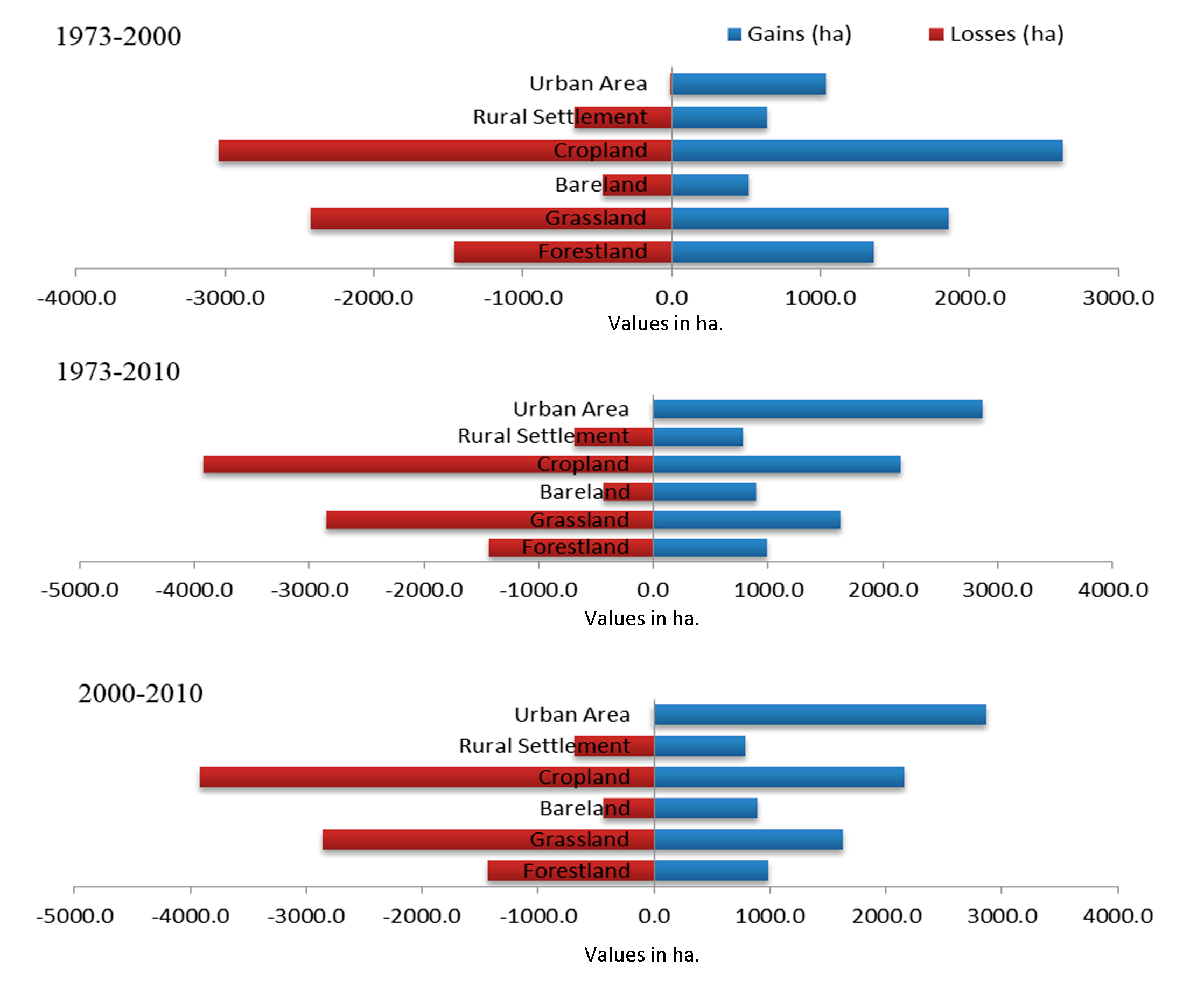
3.6 LULC Change Analysis: Gains and Losses
From 1973 to 2000, the total built-up areas increased by 1040.3ha (7.63 %) and lost by 4.2 ha (0.03 %) and net change was of 1036 ha (7.60%) while rural settlement decreased 654.4 ha (4.79%) and gained 645.8 ha with a net loss of 8.6 ha. Similarly, crop land lost was 3043.4 ha (22.32%) and gained 2629 ha (19.28%). Bare land increased by 521 ha and lost by 465.1 ha (3.411%), and net change of 55.9 ha increasing by 0.4%. Forest land decreases by 1462.7 ha (10.72%) and gained 1360.4 ha (9.977%). Similarly, grass land decreased by 2425.1 ha (Figure 7).
Figure 7.Gains and losses
3.7 Net Changes in LULC: 1973-2010
Net change is the difference between gain and loss area under different classes of LULC identified in the study area. Urban area was increased through the study periods 7.6% (1973-2000) and 13.44% (2000-2010) (Table 9) crop land which is highly converted into urban area and decreased 3.03% (1973-2000) and 12.89% (2000-2010). Bare land increased 0.4% (1973-2000) to 3.3% (2000-2010), grass land decreased from 4.15% (1973-2000) to 8.94% (2000-2010), forest land decreased from 0.75% (1973-2000) to 3.23% (2000-2010) and rural settlements has net loss of 0.06% (1973-2000) and net gain of 0.69% (2000-2010).
Table 9. Net changes of LULC: 1973-2010
LULC
Change (1973-2000)
Change (2000-2010)
ha
%
ha
%
Forest land
-102.3
-0.75
-441.5
-3.23
Grass land
-2322.8
-17.3
-1219
-8.94
Bare land
55.9
0.40
451.5
3.3
Crop land
-414.4
-3.03
-1758.7
-12.898
Rural settlements
-8.7
-0.06
94.3
0.69
Urban area
1036.
7.79
1831.9
13.43
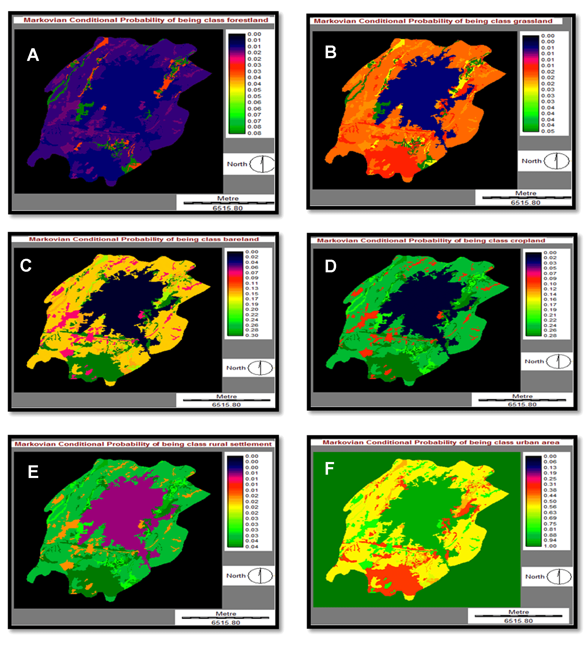
3.8 Markovian Conditional Probability Land Covers Prediction
In Markovian systems, the future state in time, t2 can be modeled on the basis of the immediately preceding state time t1. Therefore, the potential condition can be estimated not on the basis of the past but rather of the current. In the past and the future are different (Eastman, 2009). Firstly, two calibration periods i.e. 1973-2000 and 2000-2010 were correspondent and considered simulation results were pre-analyzed in terms of goodness of fit. Markov chain produces a transition matrix (Table 10), a transition area matrix (Table 11) and a set of conditional probability images by analyzing two qualitative land cover images (Figure 8) for two different periods (1973 and 2000). The transfer probability matrix (Table 10) indicates the possibility that each ground cover category will move to other categories in 2010. (Table 11) represents the number of pixels ( m) that will be converted over time from one level of land cover to another level. Markov Chain Analysis also generates similar conditional probability images (Figure 8) with the aid of transformation probability matrices. This image considered conditional since the likelihood depends on the current state. These images that have been modeled from the two previous land cover change images are useful for estimating possible land cover changes. Each conditional probability picture shows the possibility of going to another type of land cover.
Figure 8. Transition maps of LULC to forestland (a), to grassland (b), bare land (c), to crop land (d), to rural settlement (e) and to urban area (f)
Table 10. The Markov probability of changing among LULC types
Land cover classes
Forest land
Grass land
Bare land
Crop land
Rural settlements
Urban area
Forest land
0.373
0.2981
0.0161
0.2557
0.0170
0.0488
Grass land
0.1449
0.3663
0.0210
0.4197
0.0505
0.1176
Bare land
0.2643
0.1089
0.0200
0.4295
0.1066
0.0107
Crop land
0.0820
0.1746
0.0663
0.5437
0.0753
0.4591
Rural settlements
0.2215
0.0108
0.0159
0.2404
0.1185
0.4038
Urban area
0.0168
0.0064
0.0060
0.0558
0.0100
0.9734
Table 11. Cells expected to transition to different classes
Land cover classes
Forest land
Grass land
Bare land
Cropland
Rural settlements
Urban area
Forest land
19538
15557
840
13346
366
2657
Grass land
11429
28322
1625
32456
3135
1358
Bare land
3418
1431
7
8215
76
12
Crop land
12134
25841
9667
80471
11241
8751
Rural settlements
3816
192
282
4269
1926
7280
Urban area
233
0
2
192
3
33246
It is clear that most regions will be transformed into built-up areas (Table. 11). Markovian conditional probability varies up to 0.97344 and it is the highest among all forms of ground cover. This probabilistic forecast relies on the past pattern of the last 10 years (1973-2000). It can be observed from the shift detection study, most areas are transformed to built-up areas, while Markov’s conditional probability images still display the same.
4 . MODEL, SIMULATIONS AND VALIDATIONS
Findings of Markov Chain Model simulation are based on a transfer probability matrix of land-use shifts from t1 (1973) to t2 (2000). For another time, this has been the basis for projection (2010). Figure 9 (c) and (d) are the real and virtual maps of Adama City for the year 2010. This was predicted as the historical transition cycles of 1973-2000 and 2000-2010 may not be the same in the Markov Chain analysis. As seen in figure 9c, a significant part of the crop land has been turned into a rising field. While there has been a great deal of expansion of built-up areas, the transfer into other land cover groups has been constrained (Table 12).
Figure 9. LULC of 2010 actual (left) and simulated (right)
Table 12. Actual and simulated LULC map: 2010
Category
Actual map (2010)
Simulated map (2010)
Change
%
ha
%
ha
%
Forest land
1747.9
12.81
1648.1
12.11098
-0.7
Grass land
2438.9
17.89
2438
17.04345
0.7
Bare land
916.84
6.72
915
6.789489
-0
Crop land
4575.5
33.56
4580
31.56929
-0.1
Rural settlements
816.3
6
825
6.42249
0.0
Urban area
3139.8
23.02
3151
26.0643
0.0
Total
13635.24
100
13624
100
0
In the most optimal case, the change of area should be 0. The more the deviation, the less sophisticated is the model. In terms of area, it is clear that urban areas, rural settlements, crop land and bare land at almost the same. But forestland has decreased while grass land has increased. It means forest land and grass land show unexpected results in the case of quantitative analysis. The statistics presented in the validation output allow the user to distinguish the error of quantification from the error of position. The quantification error occurs where the number of cells in a category on a map varies from the number of cells in that category on the other map. Place error arises where the location of the division on one map is different from the location of the category on the other map. Thus, in addition to calculating the conventional standard Kappa index of agreement (KIA, also denoted K standard in cross table), validate offers more statistics: Kappa for no information (K no), Kappa for location (K location), Kappa for quantity (K quantity), value of perfect information of location (VPIL) and value of perfect information of quantity (VPIQ). All of these statistics are linear functions of the nine points given in the validation output (Pontius, 2000) (Table 13).
Table 13. Cross tabulation, of actual and simulated LULC map: 2010
Categories
KIA (when actual land cover map was referenced)
KIA (when simulated map was referenced)
Forest land
0.2643
0.3392
Grass land
0.2947
0.506
Bare land
0.8842
0.8925
Crop land
0.8416
0.8891
Rural settlements
0.6409
0.5766
Urban Area
0.994
0.8870
Overall Kappa: 0.884
The result of Kappa Index of Agreement (KIA) was very good for overall kappa for urban areas, crop land, and bare land moderate for rural settlement, fair for forest land and grass land. This variation occurs due to the temporal variations of satellite data. Kappa value <0.2 is poor, 0.21-0.4 is fair, 0.41-0.6 is moderate, 0.61-0.8 is good and 0.81-1 is very good (Landis and Koch, 1977). In comparing, the map of reality to the alternative map: K no indicates the overall agreement. K location indicates the extent to which the two maps agree in terms of the location of each category given the specified quantities. VPIL shows the additional percentage right to be achieved if the alternate map was
to have an ideal position due to no change in its quantity for each category indicated (Table. 14). VPIQ shows the additional percentage right to be obtained if the alternate map was to have the perfect quantity provided that did not adjust the ability to specify the position (Pontius, 2000).
Table 14. Validation of reference and simulated LULC map: 2010
Category
Ref. Prop.
Sim. Prop.
K-location
VPIL
Forest land
0.0222
0.1189
0.3492
0.0322
Grass land
0.0442
0.0100
0.4056
0.0258
Bare land
0.0796
0.6698
0.7942
0.0068
Crop land
0.2597
0.2804
0.8891
0.0282
Rural settlements
0.3318
0.0347
0.3309
0.2113
Urban area
0.3288
0.1541
0.999
0.0003
Correct chance
0.1429
Perfect chance
0.1429
Correct quantity
0.1918
Perfect location
0.6641
Correct location
0.5924
Perfect quantity
0.1830
Error location
0.0545
K number
0.9249
Error quantity
0.0184
K location
0.9337
VPIL
0.0545
K quantity
0.9633
VPIQ
0.0169
K standard
0.884
The Kappa coefficients for each division indicate large values from the above findings. This proves that there is a significant consensus between the two maps. Only forest land and grass land have a lower valuation than the average of the other groups.
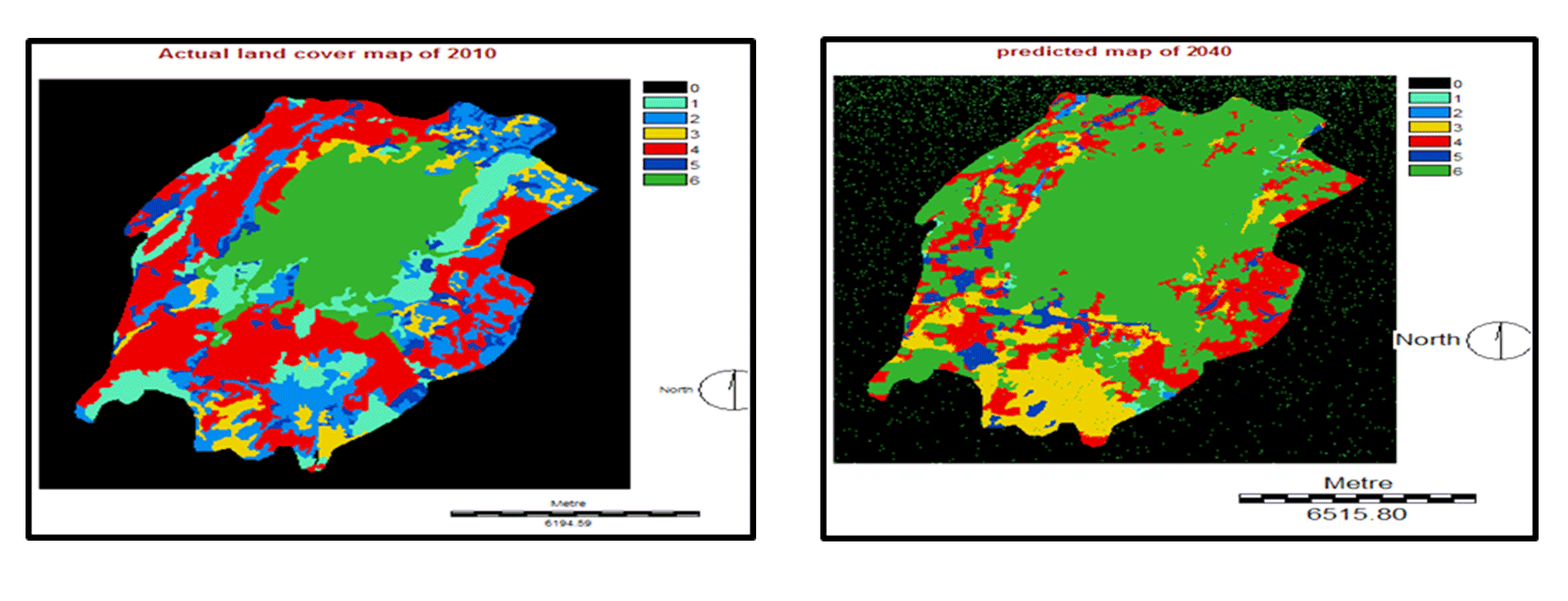
4.1 Future Prediction
In the change allocation panel which used to predict future scenarios, there are two basic models of change are provided. These are a hard prediction model and a soft prediction model. Because the soft prediction yields a map of vulnerability to change for the selected set of transitions, it is preferred to be used in this study. Thus, a map for 2010 of study area has been simulated in order to compare with the ‘actual’ land cover map of 2010. Finally, the validation panel which allows determining the quality of the prediction land use map in relation to a map of reality. It has been evaluated by running a 3-way cross tabulation between the later land cover map (a map of 1973), the prediction map (simulated map of 2010), and a map of reality (actual map for 2010). Pinto et al (2009) showed that the overall quality of land cover maps generated from model simulations should be evaluated using Kappa statistics parameter. Modeling of land use and land cover changes for future time is important to know the possible scenarios. In the case of Adama area, in order to model for future time the following assumptions were set. The modeling process for the year 2040 was depending on the assumption that the nature and developments in Adama city stayed similar to the transitions of LULC changes between 1973 and 2010.
Using Markov Chain analysis, it is possible to evaluate the transformation weights that will be used in the Markov Chain probabilities matrix for the potential projection map (Figure 10). The transition probabilities are shown in table 15, 16 and 17. The input images are LC map of 2000 and 2010 with the time difference of 10 years and 30 years.
Figure 10. Predicted LULC map: 2040
Table 15. Markov probability of changes between the LULC types
Land cover classes
Forest land
Grass land
Bare land
Crop land
Rural settlements
Urban area
Forest land
0.0116
0.0064
0.1406
0.2191
0.0318
0.5904
Grass land
0.0111
0.0071
0.1906
0.2685
0.0376
0.4850
Bare land
0.0107
0.0076
0.2970
0.2766
0.0391
0.3690
Crop land
0.0107
0.0064
0.1511
0.2470
0.0348
0.5501
Rural settlements
0.0102
0.0036
0.0744
0.0990
0.0177
0.7950
Urban area
0.0097
0.0018
0.0121
0.0150
0.0078
0.9536
Table 16. Cells transition to different classes
Land cover classes
Forest land
Grass land
Bare land
Crop land
Rural settlements
Urban area
Forest land
177
98
2142
3338
485
8995
Grass land
110
71
1891
2665
373
4813
Bare land
523
371
14506
13510
1910
18028
Crop land
1646
983
23310
38100
5369
84857
Rural settlements
228
80
1660
2209
395
17731
Urban area
881
163
1096
1356
705
86252
Table 17. LULC Changes: 2010 and 2040
LCC
Actual map of 2010
Predicted map of 2040
Change in area (%)
Area (ha)
%
Area (ha)
%
Forest land
1747.9
12.81
104.44
0.77
-3.7
Grassland
2438.9
17.89
74.30
0.55
-2.36
Bare land
916.84
6.72
1804.30
13.23
-1.08
Cropland
4575.5
33.56
2875.4
21.09
-24.16
Rural settlement
816.3
6
554.8
4.07
-2.47
Urban area
3139.8
23.02
8222.0
60.29
33.77
Total
13635.24
100
13635.24
100
0
As indicated in table 17, the ratio of built-up, areas in 2010 was 23.02% of the entire, study area. In 2040 the rate of expansion areas showed, more than double increase, and it was 60.29% of area coverage. Almost all land cover decreases from 2010 to 2040, especially crop land decreases 33.77% and forest land decreased by 3.7%, grass land and rural settlement decreased by almost the same ratio (2.36% and 2.47%), respectively and lastly bare land rarely decreased by 1.08% of the area coverage (Figure11).
Figure 11. LULC actual in 2010 (left) and predicted map for 2040 (right)
4.2 Gains and Losses in LULC
Over the years, the built-up area has risen though there is a small loss in this group. This means that some portions of the existing built-up areas have been transformed to some other land cover classes, whilst a large new region has been turned into a built-up area from the other classes of the gains, losses and longevity outcomes seen in the Table 18.
Table 10. The Markov probability of changing among LULC types
Land cover classes
Forest land
Grass land
Bare land
Crop land
Rural settlements
Urban area
Forest land
0.373
0.2981
0.0161
0.2557
0.0170
0.0488
Grass land
0.1449
0.3663
0.0210
0.4197
0.0505
0.1176
Bare land
0.2643
0.1089
0.0200
0.4295
0.1066
0.0107
Crop land
0.0820
0.1746
0.0663
0.5437
0.0753
0.4591
Rural settlements
0.2215
0.0108
0.0159
0.2404
0.1185
0.4038
Urban area
0.0168
0.0064
0.0060
0.0558
0.0100
0.9734
5 . CONCLUSIONS
Population development and the concentration of individuals in urban areas are increasing rapidly, especially in developed countries. Urban land-use and land-cover shifts have a broad variety of implications at least on a geographical and temporal scale. During this study, satellite data were used for the 1973, 2000 and 2010 periods for the providing of land-covered maps by supervised classification techniques. Accuracy evaluation and error identification procedures are also carried out. The overall accuracy of the land cover and land use maps produced during this study was of sufficient importance. Overall accuracies were 88.09% in 1973, 89.52% in 2000 and 90.95% in 2010. The accuracy of the image classification, data became, important to the modeling, process. To analyze structural shifts in built-up areas as a result of various driving forces land-use modeling was used in the last segment. The change analysis, results from the cross-tabulation also showed that built-up, areas gained 1040 ha (1973-2000) 1876.4 ha (2000-2010) and 4604.26 ha (2010-2040) and it shows rapidly changing of 2% in 1973 to 10% in 2000; 23% in 2010 to 60.27% in predicted maps 2040. Crop land areas explained the bulk of the overall increase in built-up areas (486.7ha), which represents, about 37.2% of the complete research area in 1973-2000. Rural settlements take the second, contribution to the overall increase in built-up, areas by about 301.8 ha (23.1%). Next to rural settlement, forest land takes the third contribution to the urban area by 129.6 ha (9.9% of the urban area). At the last, grass land contributes 115.2 ha (8.8% of the urban area) and bare land contributes only 7 ha (7% of the urban area). In 2000-2010, crop land areas were also continued to contribute a majority of about 102.4 ha (32.53%). Next rural settlement and forestland contribute 391.72 ha (12.47%) and 321ha (10%) of the whole study area, respectively. Grass land 130 ha (4%) and bare land 11.9 ha (0.39%) were less contributed. The conversion of crop land to build up areas might be associated with the increment of population and faster economic development in Adama city. Urban areas increased through all study periods 7.6% (1973-2000) and 13.44% (2000-2010). Crop land which highly contributes to geographical area decrease in a very net change of loss of 3.03% (1973-2000) and 12.89% (2000-2010) at this era forest land contributes to an urban area. Bare land increase 0.4% (1973-2000) to 3.3%(2000-2010), grass land decrease from 4.15% (1973-2000) to 8.94% (2000-2010) to forest land decreases from 0.75% (1973-2000) to 3.23% (2000-2010) and rural settlement has net change loss 0.06% (1973-2000) to net gain 0.69% (2000-2010). The statistics presented in the validation outputs allow the user to distinguish the error of quantification from the error of position. The kappa coefficients for each group indicate large values from the above results (K standard = 0.884). This proves that the consensus between, the two maps is important. Only forest land and grass land have a lower valuation than the sum of the opposite groups. Based on the Markov Chain Model simulation, it has been predicted that 60.27% of the total, study areas will be transformed to the built-up area cover in 2040.
Tables
Figures
Conflict of Interest
The authors declare no conflict of interest in this article.
Abbreviations
AHP: Analytical Hierarchy Analysis; APO: Adama Project Office’s; CA: Cellular Automata; CORINE: Co-ordination of Information on the Environment; CSA: Central Statistical Agency; EEA: European Environment Agency; ETM: Enhanced Thematic Mapper; GCP: Ground Control Point; GIS: Geographic Information System; GPS: Global Positioning System; KIA: Kappa Index of Agreement; LC: Land Cover; LULC: Land Use Land Cover; MSS: Mobile Satellite Services; NLFS: National Labor Force Survey; PRB: Population Reference Bureau; RS: Remote Sensing; UN: United Nation; UTM: Universal Transverse Mercator; VPIL; Value of Perfect Information of Location; VPIQ: Value of Perfect Information of Quantity; WGS: World Geodetic System.
Africover, 2002. Specifications for geometry and cartography: A summary report of the workshop on Africover.
3.
Al-Shalabi, M. A., Bin Mansor, S., Bin Ahmed, N and Shiriff, R., 2006. GIS-based multi-criteria approaches housing site suitability assessment. In XXIII FIG Congress, shaping the change, Munich, Germany, October, 8-13.
Eastman, J. R., 2009. IDRISI Taiga guide to GIS and Image Processing (Manual Version 16.02) [Software] (Massachusetts, USA: Clark Labs, Clark University).
Herold, M., Menz, G. and Clarke, K. C., 2001. Remote sensing and urban growth models- demands and perspectives. In symposium on remote sensing of urban areas, Regensburg, Germany, Regensburger Geographische Schriften, 35.
29.
IDRISI Taiga Help System, 2009. Clark Labs, Clark University, 950 Main Street, Worcester, MA01610-1477, USA.
30.
Keil, R., 2018. Suburban Planet. Making the World Urban From the Outside, Polity Press, Medforg, MA, USA.
Pinto, P., Cabral, P., Caetano, M and Alves, M. F., 2009. Urban growth on coastal erosion vulnerable stretches. Journal of Coastal Research, 2, 1567-1571.
Tadesse, W., Coleman, T. L, and Tsegaye, T. D., 2003. Improvement of land use and land cover classification of an urban area using image segmentation from Landsat ETM+ data. In Proceedings of the 30th international symposium on remote sensing of the environment, 10-14.


 ,
Mikir Kassaw 2
,
Mikir Kassaw 2
 m) that will be converted over time from one level of land cover to another level. Markov Chain Analysis also generates similar conditional probability images (