3.1 Master Recession Curve using a Reservoir Linear Model

Recession segments were selected in the linear reservoir model calibration of 57 individual recession segments. These were selected recession segments with relatively small RMSE model errors representing each year during the study period. The recapitulation results of recession parameters and recession discharges include duration, recession coefficients and constants, observational recession discharges and model recession discharges and model errors (RMSE). The duration of recession events during the period from 2000 to 2010 ranged from 11-21 days. The recession parameters combination for the initial recession discharge (Q0) ranges from 1.71-4.95 m³/sec with an average of 3.14 m³/sec, the recession coefficient (k) ranges from 0.06-0.15 with an average of 0.10; and the recession constant ranged from 0.861-0.941 with an average value of 0.907. The observational recession discharge calculation goes from 0.75-2.73 m³/sec with an average of 1.79 m³/second, and the model recession discharge calculation ranges from 0.82-2.74 m³/ecs with an average of 1.82 m³/s and the model error (RMSE) ranges from 0.0116-1.1133 with an average of 0.1775 as presented in Table 4.

The linear reservoir model calibration results for the study area can be compared with the results of baseflow recession research in some regions. The study results (Moore, 1997) analyzed simulated a baseflow recession for linear, exponential reservoirs, namely two parallel linear and two serial linear. The results showed that the double-reservoir model was substantially effective compared to a single setting. However, based on the recession segment pattern for the linear and exponential reservoir model, the suitability for the recession model is relatively consistent depending on the number of parameters and the flexibility of the resulting recession function. Calibration of the double reservoir model performs very well than linear reservoirs using the quadratic difference loss function.

3.1.1Visualize MRC Manually using a Linear Reservoir Model

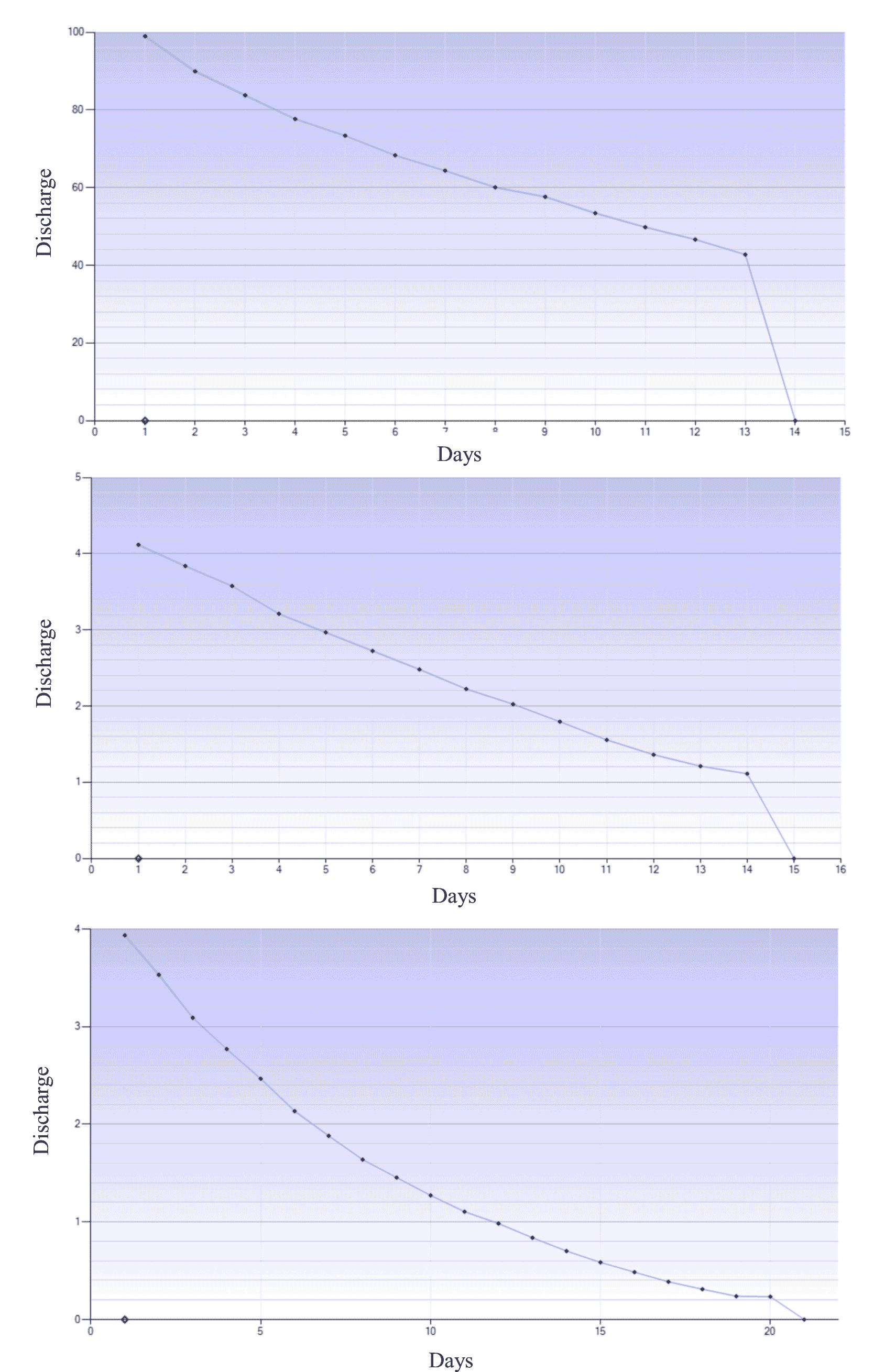
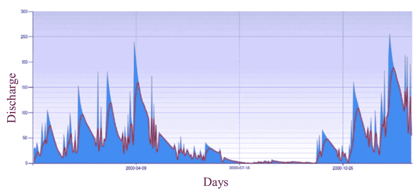
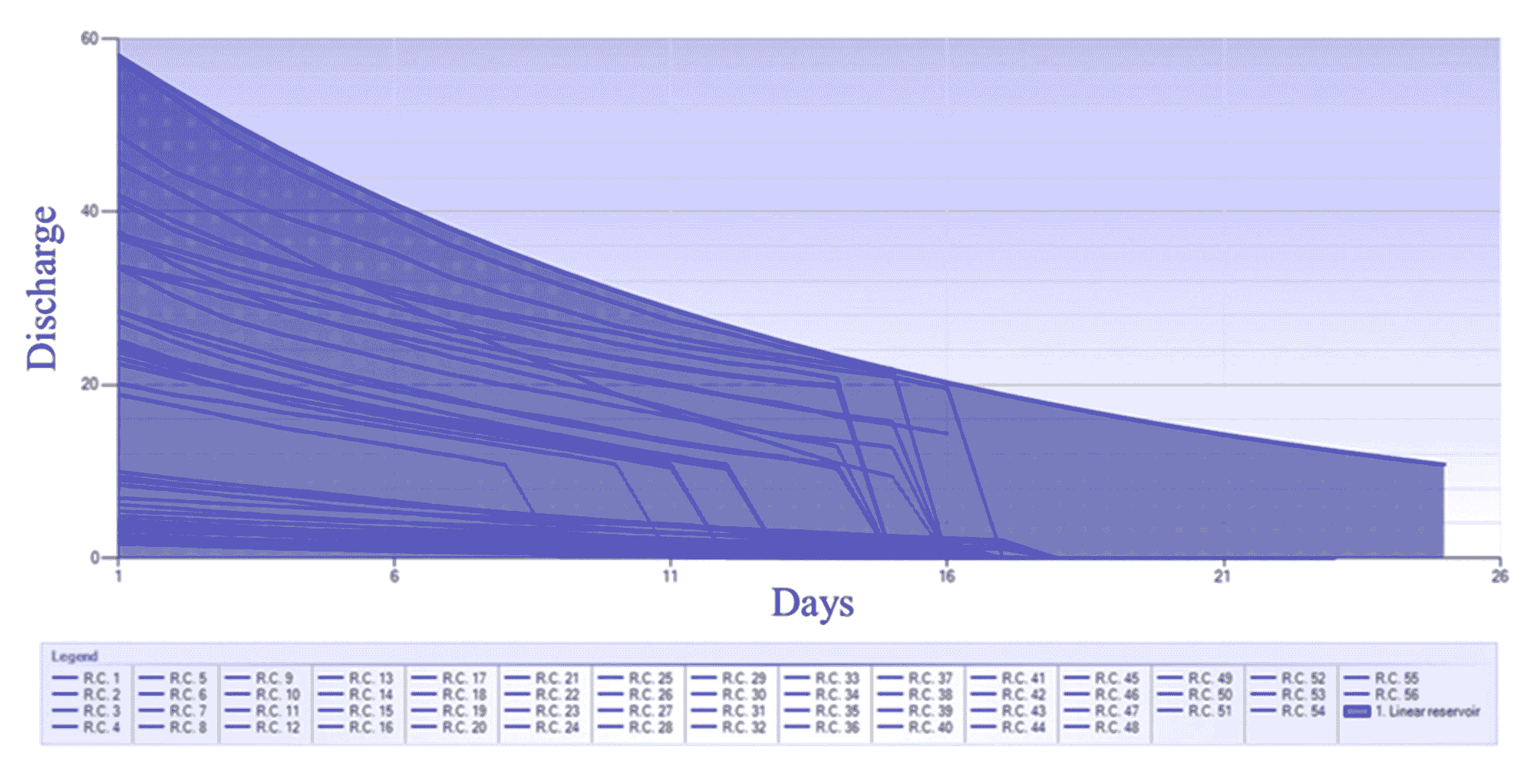
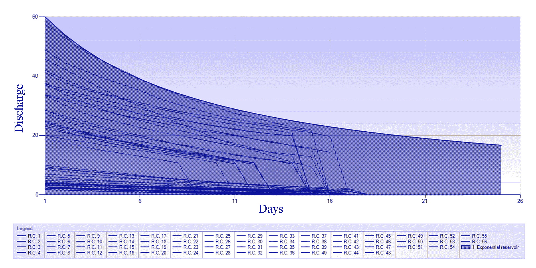
Visualization of recession and recession discharge parameter calculations for the research period was then further analyzed using a linear reservoir model to obtain a master recession curve manually and a process-based genetic algorithm. A visualization of the master recession curve for the research watershed is presented in Figure 5.

Figure 5. Visualization of MRC manually for linear models

The series of recession segments shows a series of recession events in the research area ranging from the duration of the recession event to the shape of the slope of the recession curve, which then reflects the characteristics of the recession in the study area. Analyzing the characteristics of a baseflow recession is indispensable for prolonged recession duration, resulting in an optimal recession curve. The recession curve is short, containing only limited information regarding the recession process and the end of time that often occurs. To solve this problem, the master recession curve method is used to measure the recession characteristics of the research watershed. The recession’s parameters and coefficients represent the baseflow recession analysis’s linearity and non-linear aspects. Variations in individual recession curves in watershed research suggest that the Q0 initial parameters of a single recession event represented by peak discharges appear to influence the shape of the recession curve. Recessionary events with a more significant peak discharge result in a recession curve that tends to shift to the right, compared to a smaller peak discharge, as seen in the visualization of the master recession curve. This is because the recession phase is the stage where the contribution of subsurface flows is dominant. Hence, the recession parameters significantly affect the shape of the baseflow recession curve. The variation in the shape of the recession curve is determined mainly by selecting the type of recession model, the determination of the parameters’ value, and the recession’s coefficient (Latuamury, 2020).

3.1.2 Hybridization of Genetic Algorithms for Visualization of MRC Linear Reservoir Models

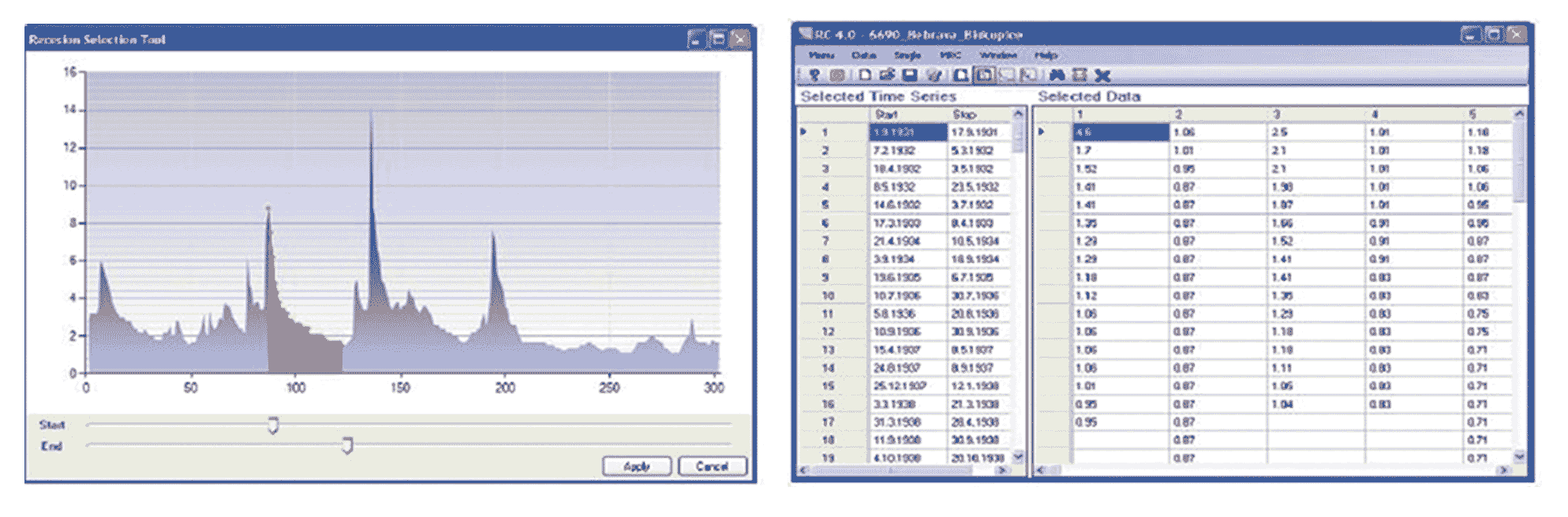
Hybridization of MRC through the process of genetic algorithms (generation) requires several stages to be determined, namely the determination of specific components, including the stability of the number of generations (NG) and individuals (NI), the maximum length of the master recession curve (ML MRC), and the optimal dispersion of mutations. This arrangement includes the optimal use of four evolution cycle parameter values NG 50, NI 10, cross probability 0.90, the maximum length of the recession master curve 50, and mutation 10 for the study area.

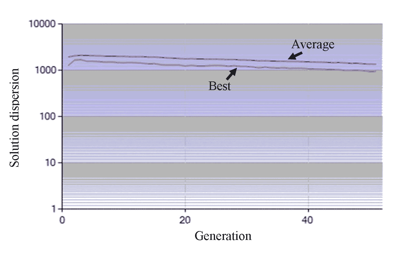
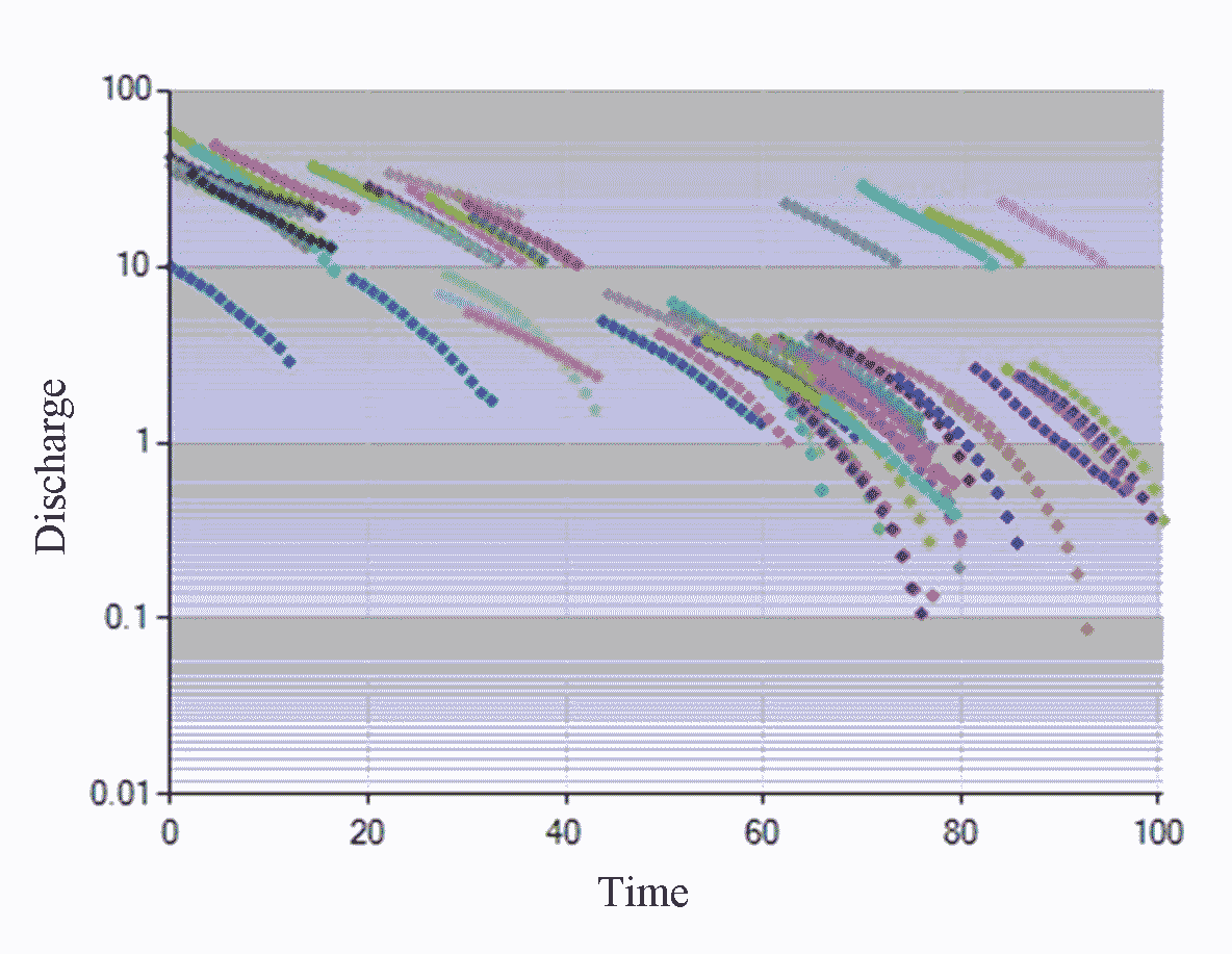
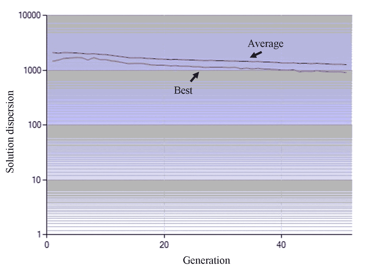
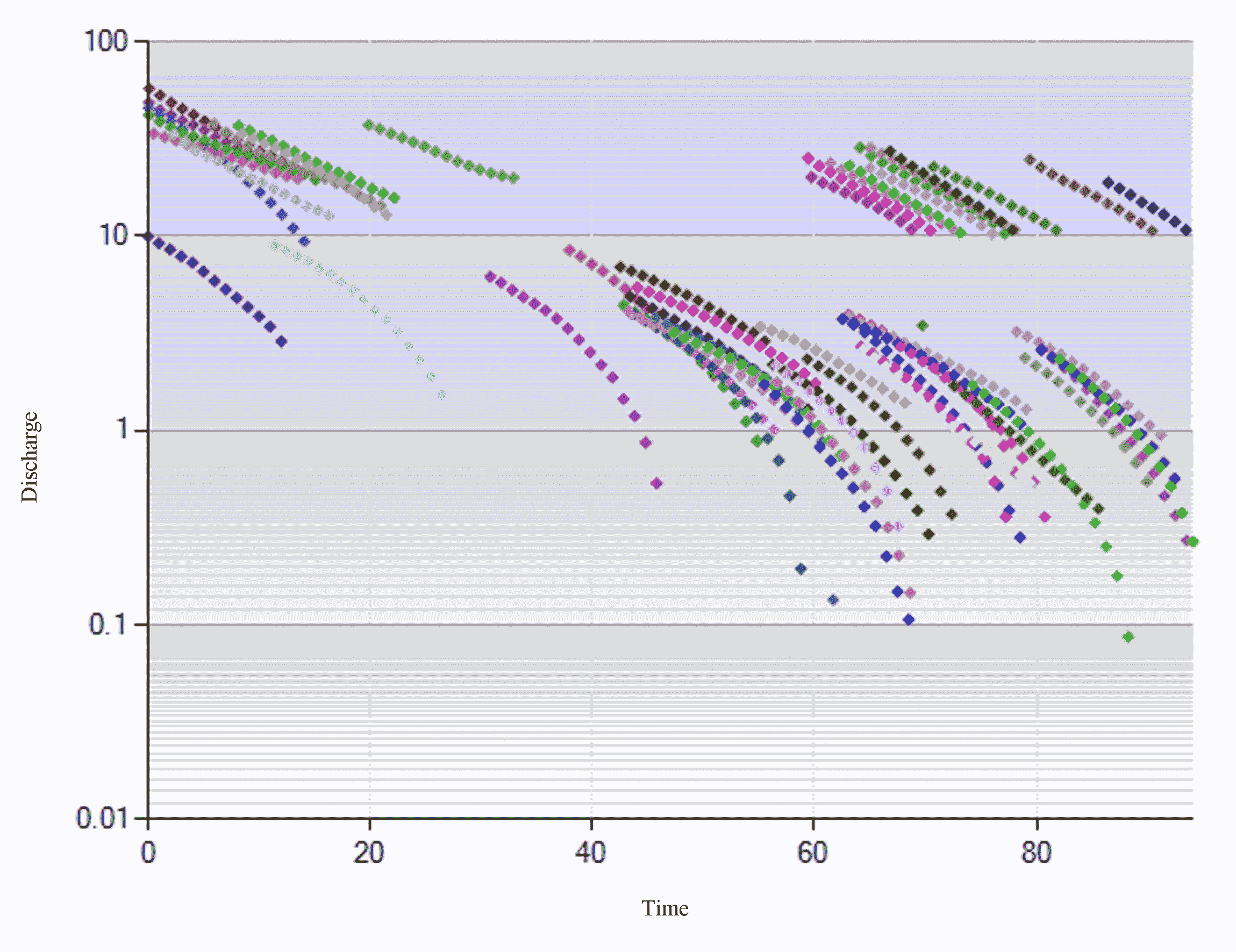
MRC visualization of genetic algorithms begins with the evolutionary process of dispersion, the best solution to produce an optimal MRC, as shown in Figure 6 and 7.

Figure 6. Visualization of logarithmic evolutionary processes for linear

Figure 7. Visualization of the best logarithmic solution process for linear

The process of hybridization of genetic algorithms through the best solutions shows the distribution of recession segments. The optimal performance of the algorithm for the Duang watershed shows a relatively similar and stable trend. However, data distribution tends to shift and accumulate towards the right. This dispersed performance is optimal for the characteristics of the recession segment, which are known to be relatively similar. Therefore, the calibration of linear and exponential reservoir models determines the coefficients and parameters of the master recession curve.

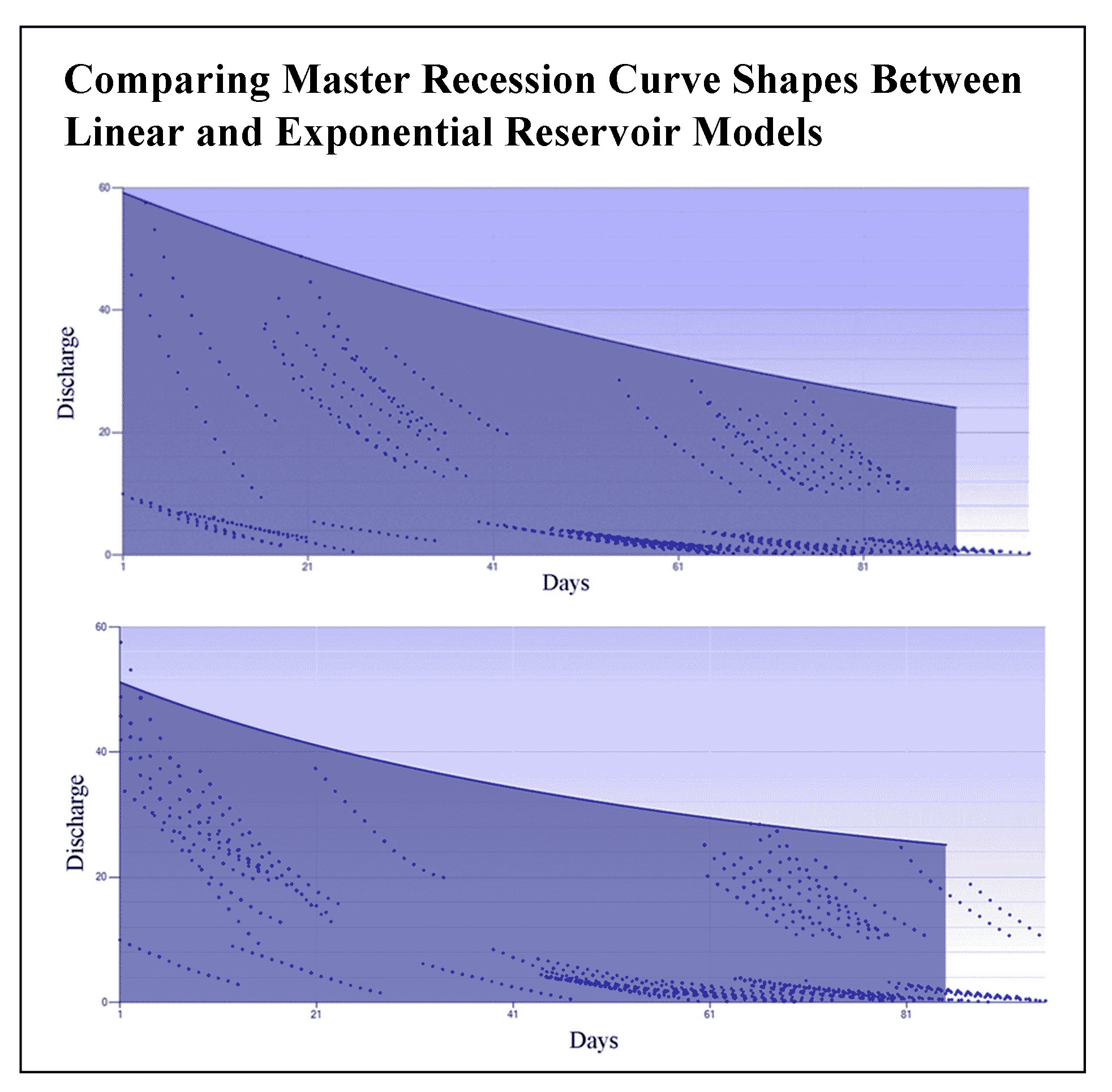
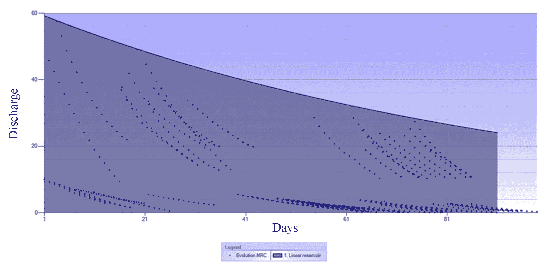
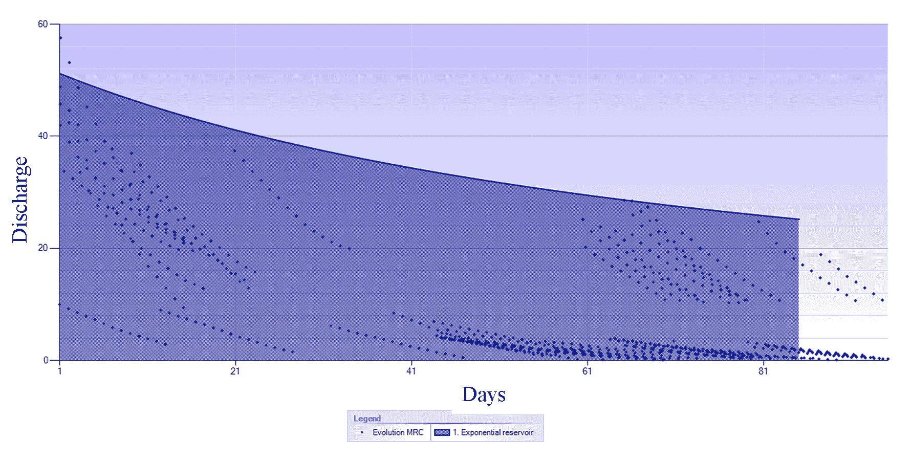
The results of MRC calibration through hybridization of genetic algorithms for linear reservoir models describe the shape and slope of the MRC determined based on a combination of recession parameters for the calibration of linear reservoir models. The variety of linear reservoir model parameters for MRC resulting from the hybridization of genetic algorithms obtained an average recession discharge Q0 of 59.18 m³/s, a recession coefficient (k) of 0.010 and a recession constant of 0.990. The results of the linear reservoir model calibration for the genetic algorithm hybridization process show that the MRC indicates that the slope of the MRC for the linear reservoir model is gentler compared to the exponential reservoir model, as presented in Figure 8.

.

Figure 8. Visualization of MRC processes genetic algorithms for linear reservoir models

3.2 Master Recession Curve Using Exponential Reservoir Model

Calibration of the exponential reservoir model used 57 individual recession segments and then selected 11 individual recession segments representing the study period with the smallest RMSE model error value estimate. The results of the recapitulation of recession parameters and recession discharges obtain variations in the duration of the recession (in days), the coefficients and constants of the recession, the observational recession discharge, and the model recession discharge as the minor model error (RMSE). The duration of recession events during the period from 2000 to 2010 ranged from 11-21 days, with an average duration of 16.5 days. The combination of recession parameters for the initial recession discharge (Q0) ranges from 1.71-4.44 m³/second with an average of 2.96 m³/sec, the recession coefficient ranges from 0.00-0.12 with an average of 0.05; and the recession constant ranges from 0.064-0.212 with an average value of 0.130. The calculation of observational recession discharge ranges from 0.76-2.29 m³/sec with an average of 1.54 m³/sec, and the calculation of model recession discharge ranges from 0.82-2.52 m³/sec with an average of 1.69 m³/second and model error (RMSE) ranging from 0.1215-0.4558 with an average of 0.2730 as presented in Table 5.

3.3 Manually MRC Visualization Exponential Reservoir Models

The results of manual calculations of a combination of recession parameters for exponential models obtained an average initial recession value Q0 of 59.990, a value of φ calibration parameter of 0.002, and a recession constant of 0.120. MRC visualizations for both reservoir models are presented in Figure 9.

Figure 9. Visualization of MRC manually for exponential reservoir models

Manual MRC visualizations for both reservoir models based on recession parameters show variations in MRC slope for both reservoir models. The slope of the MRC for the linear reservoir model is gentler than the exponential reservoir model. The slope of the MRC is very closely assembled with the combination of recession parameters from the calibration results of both models, that the recession parameters for the linear reservoir model are higher than the exponential reservoir model.

3.4 Hibridisasi Algoritma Genetika Untuk Visualisasi MRC Exponential Reservoir Models

The MRC assembly stages through hybridization of the genetic algorithm process follow the same stages as the generated assembly for linear reservoir models, i.e., the number of generations (NG) and individuals (NI), the maximum length of the recession master curve (ML MRC), and the optimal mutation dispersion. The four parameters of the optimization of the evolutionary cycle parameters are NG 50, NI 10, cross probability 0.90, the maximum length of the recession master curve 50, and mutation 10. The calibration results of the MRC exponential reservoir model from the hybridization of the genetic algorithm process through the evolutionary process of dispersion, the best solution, obtaining the optimal MRC, as presented in Figures 10 and 11.

Figure 10. Visualization of logarithmic evolutionary processes for exponential models

Figure 11. Visualization of the best logarithmic solution process for exponential reservoir models

The best solution of hybridization MRC results through a genetic algorithm process shows the distribution of recession segments and optimal algorithm performance for research areas with relatively stable trends. Distributed performance is optimal for somewhat similar recession segments. Further, calibration of the exponential reservoir model establishes the parameterization of the MRC, as presented in Figure 12.

Figure 12. Visualization of MRC processes genetic algorithms for exponential reservoir models

The combination of recession parameters for the calibration of the exponential reservoir model obtained an average initial discharge of recession (Q0) of 51.19 m³/s, a recession coefficient (φ) of 0.00024, and a recession constant of 0.0120. The results of calibration calculations for exponential reservoir models using hybridization of genetic algorithms show that linear reservoir models have a higher recession initial discharge compared to exponential reservoir models. Recession parameters for both reservoir models show that the MRC slope for the linear reservoir model is more gentle compared to the exponential reservoir model as presented in Figure 12.

The results of the master recession curve visualization using the genetic algorithm process of the two reservoir models showed that the linear reservoir model had a gentler slope than the exponential reservoir model. This result gives a difference between the two models due to the recession parameters combination, the recession constant, and the coefficient of each model. Recession parameters for linear reservoir models are higher than for exponential reservoir models. The combination of recession parameters for both reservoir models results in a master recession curve of the genetic algorithm process that is more significant for both models. The recession constant and coefficients combination shows a visualization of a relatively flattened master recession curve for linear reservoir models and relatively steeper exponential reservoir models than linear reservoir models. The slope of the master recession curve for both reservoir models will determine the flow storage capability and also the nature of hydraulic conductivity for both reservoir models. The gentle slope of the master recession curve has a relatively slow storage nature, while the steep slope of the master recession curve determines the somewhat wasteful nature of storage. The storage properties of groundwater are also closely related to hydraulic conductivity and the characteristics of the catchment area in the surface flow. The calibration results of the linear and exponential reservoir models and the parameterization of the initial recession discharge, recession coefficients, and constants, and the observational recession discharge and recession model are closely related to the characteristics of the study area matched with the results of research in the catchment area in several countries among others (Boughton, 2015) developed a master computer program to build the latest MRC from the daily discharge records of 100 river measurement stations in Australia. Substantial variations of the recession segment show significant variations in the baseflow recession of the simple exponential decay model. The differences in theoretical exponential decay models and baseflow recessions are assumed due to various transmission losses. The average value of the recession segment in the recessionary period derives from the MRC of a more straightforward set of recession segments compared to the previous method. The transmission loss estimation method relies on the bottom flow recession segment within the MRC, so this method is not suitable for ephemeral rivers in semi-arid areas but is more suitable for assessing transmission losses in humid zones.

The baseflow in many rivers often come from streams from shallow groundwater aquifers. This assumes that many algorithms show that aquifer outflows are disproportionately linear to flow storage (Wittenberg, 1999). The alternative hypothesis is that nonlinear reservoir functions are relatively more realistic than linear reservoir functions (Moore, 1997; Lin et al., 2007). A relatively rapid response, especially from groundwater flow and precipitation, results from the hydraulic head of the groundwater reservoir, which accelerates exfiltration and outflow to the baseflow (Hannah and Gurnell, 2001; Aksoy and Wittenberg, 2011; Chen et al., 2012). When pore pressure and volume are hydraulically related, a single nonlinear reservoir model makes sense for a particular catchment area or an independent parallel linear reservoir (Bonacci, 1993; Peters et al., 2005). The nonlinear reservoir algorithm uses an analytical derivation model in the automatic separation of the bottom flow from a series of daily discharge times from the river and the practical calculation of groundwater storage and watershed replenishment in the inversion of nonlinear reservoirs.

A comprehensive and objective approach to analyzing base flow recessions with recession innovations uses quantitative regression and efficient and accurate numerical estimation, including groundwater intake curves. Thomas (2012) introduced one of the innovations of quantitative regression models (Stoelzle et al., 2013), drawing the distribution of baseflow recession data within the lower limit of the hydrographic recession curve. The use of quantitative regression presents a rigorous and reproducible method of estimating recession parameters and a traditional subjective approach, resulting in the best model. The second innovation estimates the derivation time of the dQ/dt recession curve by comparing six estimators from more efficient algorithms for estimating baseflow recession parameters. The third innovation considers seasonal variations in baseline flows across various recession parameters that are statistically significant across all seasons. Wang and Cai (2010) introduced the fourth innovation by considering groundwater intake parameters into baseflow recession analysis. Thomas et al. (2015) The nonlinear response of recessionary behavior increases as groundwater intake increases, thus considering the availability of groundwater collection data on a similar regional scale (Mizumura, 2005;  Aksoy and Wittenberg, 2011; Collischonn and Fan, 2013).

The authors declare that there is no conflict of interest.

The authors are grateful to the leaders and staff of the Surakarta River Watershed Research and Technology Center, Ministry of Environment, and Forestry, for the daily data provision needed to complete this research.

MRC: Master Recession Curve; NG: Number of Generations; NI: Individuals; Rb: Bifurcation Ratio; Rc: Circulation Ratio; VBA: Visual Basic for Applications.