3 . METHODOLOGY
3.1 Data Sources
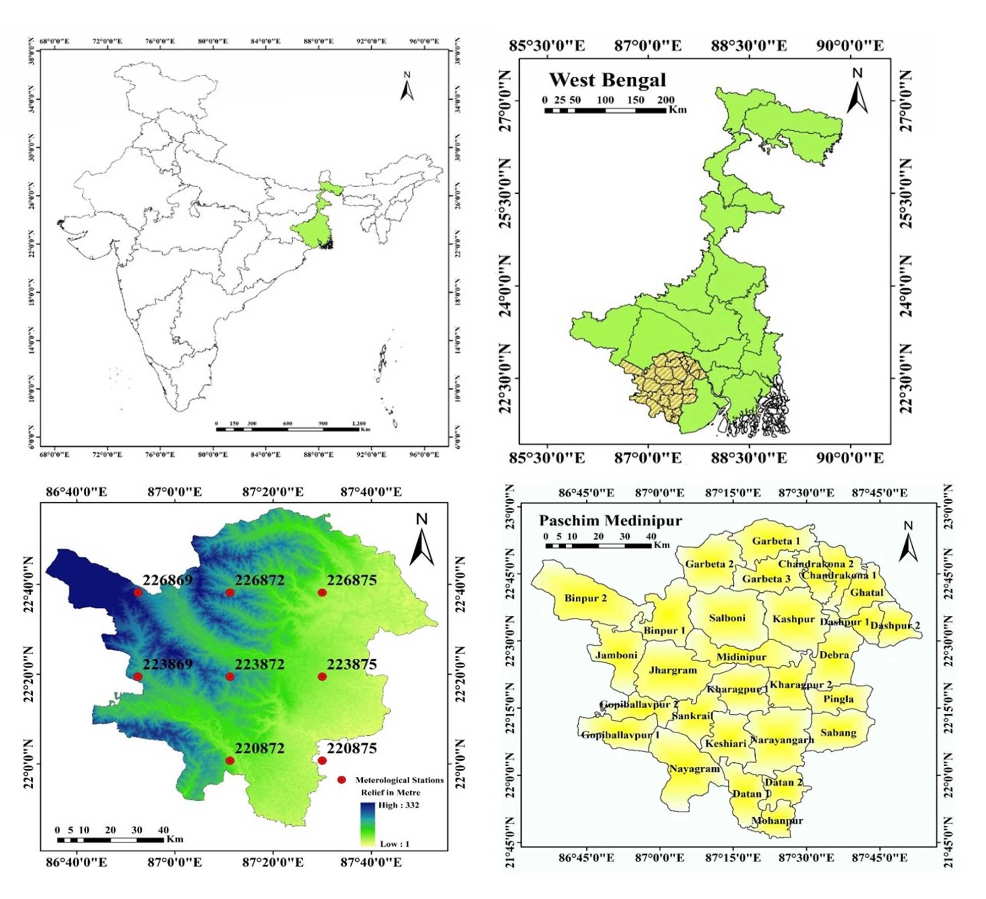
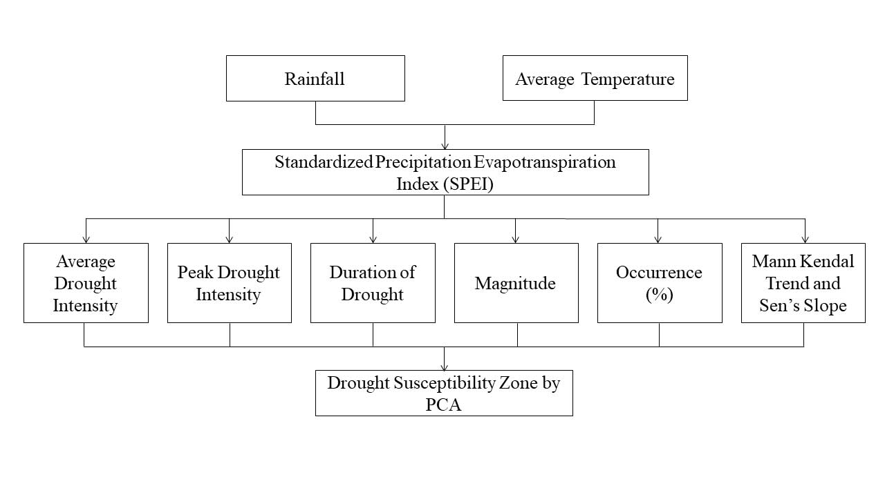
One of the most popular, reliable and adaptable dataset for identifying and monitoring droughts is CFSR (Sommerlot, 2017). CFSR data depends on both historical and operational archives of observations (White et al., 2017). Since 1978, many satellite missions are combined from CFSR assimilation which is from the archive of National Centres for Environmental Prediction (NCEP), European Centers for Environmental Prediction (ECMWF), Japan Meteorological Agency (JMA), United States Air Force (USAF) and African Monsoon Multidisciplinary Analysis (AMMA) (Dile and Srinivasan, 2014). Being the first reanalysis system to use the 6-hour prediction from a linked atmosphere-ocean climate system with an interactive sea ice component as the guess fields gives CFSR its singular advantage (Yu et al., 2011). The station data that is provided in the SWAT format at https://swat.tamu.edu/data/cfsr is created from the reanalysis datasets. These daily station data are extracted for our investigation and transformed to monthly values. The list of meteorological stations is shown in Table 1 together with their latitude, longitude, mean rainfall and standard deviation of rainfall. This study considers continuous rainfall data from 8 meteorological stations. Figure 1 shows where the meteorological stations are located in West Bengal’s Paschim Medinipur District. The overall methodological structure of this study is depicted in Figure 2. From rainfall and mean temperature, SPEI has been estimated. Based on SPEI intensity, magnitude, trend, duration and occurrence rate or frequency (%), are estimated at 3, 6, 12- and 48-months’ time step. The above-mentioned parameters are used to assess PCA at different time steps which is used to drought susceptibility zones of the study region.
Table 1. Meteorological stations
|
Stations
|
Longitude
|
Latitude
|
Elevation(m)
|
|
220872 (1st Station)
|
87.1875
|
22.0121
|
22
|
|
223872 (2nd Station)
|
87.1875
|
22.3244
|
66
|
|
223875 (3rd Station)
|
87.5
|
22.3244
|
12
|
|
226869 (4th station)
|
86.875
|
22.6366
|
86
|
|
223869 (5th Station)
|
86.875
|
22.3244
|
73
|
|
226872 (6th Station)
|
87.1875
|
22.6366
|
63
|
|
226875 (7th Station)
|
87.5
|
22.6366
|
15
|
|
220875 (8th Station)
|
87.5
|
22.0121
|
9
|
3.2 Drought Evaluation Parameters (Dp)
Drought evaluation parameters are necessary to analyze drought in a meticulous way (Caloiero, 2018). Dracup et al. (1980) measured several drought related parameters such as intensity, frequency or occurrence rate, duration and trend of drought at several time steps. The manuscript follows almost same guideline to illustrate spatiotemporal assessment of meteorological drought:
3.2.1 Estimation of drought using Standardized Precipitation Evapotranspiration Index (SPEI)
According to Vicente-Serrano et al. (2010) and Beguera et al. (2013), the SPEI is based on temperature and precipitation data and has the advantage of integrating multi-scalar character with the ability to account for the effects of temperature fluctuation on drought evaluation. A climatic water balance, the accumulation of deficit/surplus at various time scales and adjustment to a log-logistic probability distribution are all steps in the process of calculating the index. The SPEI is mathematically comparable to the Standardized Precipitation Index (SPI), but it also takes temperature into account. The Palmer Drought Severity Index can be compared to the SPEI because it is based on a water balance (PDSI).
The SPEI generally utilizes monthly or weekly differences of rainfall and potential evapotranspiration (Thornthwaite, 1948). This phenomenon indicates a simple climatic water balance that can be calculated in different time steps which indicate SPEI. The first step of calculating SPEI involves the calculation of Potential Evapotranspiration (PET). Here the simple approach of Thornthwaite (1948) has been followed. The method has a great advantage that the method requires only the monthly mean temperature data. The monthly PET for this study is computed as follows:
\(PET= 16K({10T \over I})^m\) (1)
Where, T is the monthly mean temperature (°C), I is the heat index which is calculated as the sum of 12 monthly index values I, now the I is derived as following:
\(I= ({T \over 5})^{1.514}\) (2)
With the value of PET, the difference between the rainfall (P) and potential evapotranspiration (PET) for the month of i is calculated using following formula
\(D_i=P_i-PET_i\) (3)
The equation (3) gives the simple measure to estimate the surplus and deficit of the specific analyzed month.
In the next step of the SPEI formation D value is calculated in different time steps. The procedure of calculation of D is as follows:
\(X_{i,J}^K=∑_{l=13-K+l}^{12}D_{i-1J}+∑_{i=1}^j D_{iJ} \ if \ j<k \ and \ X_{i,J}^K=∑_{l=j-k+1}^j D_{i,l} \ {if} \ j≥k\) (4)
The equation (4) represents the total difference over one month in a certain year i using a 12-month time frame. The P-PET difference in millimeters during the first month of the year is represented here by Di. Depending on the time scale k used.
The series D has negative values so two parameters gamma distribution function cannot be fit for this series. Thus, three parameters gamma distributions have been used. In the three parameters gamma distribution x can take values in the range ( \(\gamma\) >D<\(\infty\)) where, \(\gamma\) is the parameter of origin of the distribution; consequently, x can have negative values which is common in the D series. After examining the 3-parameters gamma distribution function Vicente Serrano (2010) concluded that the log-logistic distribution is the best fit on the x series values. The form of the density function of the 3-parameters log-logistic distribution is expressed as follows:
\(f(x) = {β \over α} ({ x- \gamma \over α}) ^{β-1} [1+ ({ x- \gamma \over α})^β]^{-2}\) (5)
Where, α, β, \(\gamma\) are shape, scale and origin parameters respectively for D values ( \(\gamma\) >D<\(\infty\)). Here, x is the cumulative series of D values in a time window which is specified here as 1979-2014. The parameters of this function are obtained using the L moment method:
\(β = {2w_1-w_0 \over 6w_1-w_0-6w_2}\) (6)
\(α= {(w_0-2w_1)β \over ϊ(1+{1\overβ})ϊ(1-{1 \over β})}\) (7)
\(\gamma = w_0-α ϊ {(1+{1\overβ})ϊ(1-{1 \over β})}\) (8)
Where, \(ϊ \) is gamma function and the probability weighted moments are w0, w1, and w2. The equation (9) calculates the log-logistic cumulative distribution function is converted to the SPEI (10) using the Abramowitz and Stegun (1964) approximation of the standard normal distribution.
\(F'(x)= {1+ ({α \over x- \lambda})}\) (9)
\(SPEI=W- {C_0+C_1 W+C_2 W^2\over 1+d_1 W+W^2 d_2+w^3 d_3}\) (10)
Where, \(C_0,C_1,C_2,d_1,d_2\) and \(d_3\) are the constants in the SPEI equation constants and W is the obtained in the following equation (11):
\(W= \left\{ {\sqrt{-2In(P)} \over \sqrt{-2In(P-1)}} \right\} \) for \(p ≤ 0.5\), p>0.5 (11)
Where, P = 1- F(x). This index is able to monitoring drought with great amusement. Table 2 determines the category of drought and their respective ranges.
Table 2. Drought severity classes based on SPEI
|
Severity Class
|
Nature of Drought
|
|
<-2.0
|
Extremely dry
|
|
-1.5 to -1.99
|
Severely dry
|
|
-1.0 to -1.49
|
Moderately dry
|
|
-.99 to .99
|
Near Normal
|
|
1.0 to 1.49
|
Moderately Wet
|
|
1.5 to 1.99
|
Very Wet
|
|
>2.0+
|
Extremely Wet
|
3.2.2 Parameters Used in Drought Risk Assessment
This study considers peak intensity, magnitude, average drought intensity, duration, occurrence rate and trend for evaluation of meteorological drought. Peak intensity (PID), magnitude (MD), average intensity (AID), duration, occurrence rate and trend are proportionately related with sensitivity of drought. Trend of drought is inversely related to drought sensitivity. The description of parameters is as follows:
3.2.2.1 Drought Intensity (ID)
According to Dupigny-Giroux (2001), drought intensity can be defined as the departure (down) of a SPEI from its typical value. A drought event, as described by Abbasi et al. (2019), is a time period during which the SPEI is consistently negative and the SPI achieves a value of -1.0 or less. Therefore, ID here signifies the SPEI value that is smaller than 1.0. The intensity of the drought will increase as SPI value decreases.
3.2.2.2 Duration of drought (DD) using Run Theory
Spinoni et al. (2014) use run theory to precisely quantify the length of a drought. When the SPEI is constantly negative and reaches to intensity of -1.0 or below, a drought event begins and it ends when the SPEI turns positive. Therefore, the continuous negative dimension of SPEI represents the length of the drought (Abbasi et al., 2019).
3.2.2.3 Magnitude (MD) and average intensity (MID) of drought
According to Thompson (1999), drought magnitude refers to the cumulative water deficit into the drought period. The average of this cumulative water deficit is the MID. Thus, MD is the sum of all SPEI values during the drought event and MID of a drought event refers to the magnitude of drought divided by the duration of the drought.
\(M_D=∑_(i=1)^n SPEI_{ij} \) (12)
\(M_D=∑_(i=1)^n SPEI_{ij} /m\) (13)
Where, SPEIij are the SPEI values of drought and wet event in j-th time and m is the number of months.
3.2.2.4 Occurrence rate (%) or frequency of drought (FD)
The number of droughts per 35 years calculated using following formula (Ghosh, 2019):
\(F_{Dj,35} = {M_j \over J.m} \times 100\) (14)
Where, FDj,35 is the frequency of droughts for timescale j in 35 years; Nj is the number of months with droughts for time scale j in the n-year set; j is time scale (3-, 6-, 12-, 48-months); n is the number of years in the data set.
3.2.2.5 Mann Kendall trend test
There are numerous statistical techniques available for identifying trends and each technique has strengths and weaknesses (Nikzad Tehrani et al., 2019). Finding the trend of meteorological variables can be done using the Mann-Kendall statistical test (Halder et al., 2020). Here, the tendency of a meteorological drought based on SPI is indicated by the Mann-Kendall trend test. One type of non-parametric test, the Mann Kendall test, is unaffected by the extremes of the sample points (Abeysingha and Rajapaksha, 2020). The World Meteorological Organization recommends the Mann-Kendall test (Mann, 1945; Kendall, 1975) and this approach is employed in the following way:
\(S=∑_{i=1}^{n-1}∑_{j=i+1}^n sgn(x_j-x_i)\) (15)
Where, n is the number of data points, xi and xj are the data values of the separate time series i and j (j>i) respectively, and \(sgn(x_j-x_i)\) is the sign function
\(sgn(x_j-x_i ) = \left\{ \begin {matrix} +1 \ if \ x_j-x_i>0 \\ 0 \ if \ x_j-x_i=0 \\ -1 \ if \ x_j-x_i=0 \end{matrix} \right \} \) (16)
The variance is computed as following:
\(Var(S) = {n(n-1)(2n+5)-∑_{i=1}^p t_i (t_i-1)(2t_i+5) \over 18}\) (17)
The summation sign denotes the sum of all tied groups, where n is the number of data points and P is the number of tied groups. The standard normal format of Zs can be computed in cases where the sample size is greater than 30, as shown below:
\(Z = \left\{ \begin {matrix} {s-1 \over \sqrt{var(s)}} \ if \ s>0 \\ 0 if \ s=0 \\ {s-1 \over \sqrt{var(s)}} \ if \ s>0 \end{matrix} \right \} \) (18)
Negative Zs value shows a positive tendency of drought, while positive Z value suggests a negative trend. Trends are tested using a defined degree of significance. When the null hypothesis is rejected, a substantial trend in the data series is present.
In the ARCGIS 10.2.2 environment, the Inverse Distance Weightage Method (IDW) has been used to visualize geographic maps.
3.2.2.6 Sen’s Slope estimator
The magnitude of trend in SPI time series was estimated in the following way (Theil, 1950; Sen, 1968):
\(β=median {X_i-X_j \over i-j}\) V \( j<i\) (19)
In the above equation (15), 1 < j < i < n. The β is the median over all combination of all recorded pairs (Tabari et al., 2011) thus does not affected by the extreme values in the observations.
3.3 Drought Susceptibility zone assessment by Principal Component Analysis (PCA)
One of the best and most widely used methods for calculating drought risk zones is Principal Component Analysis (PCA) (Cai et al., 2015; Dinpashoh et al., 2004). According to Demar et al. (2013), PCA is a multivariate technique that lowers the dataset’s dimensionality by computing a collection of new orthogonal variables in decreasing order. In order to estimate principal components, the research used Jolliffe’s (2002) method. In this work, the estimation of the principal components is done in time steps of 3, 6, 12 and 48 months. X is taken to be a vector made up of p random variables in this instance.
PCA is focused with the association and covariance in this investigation. A vector of p constants, such as α11, α12, . . ., α1p, and α′ is one of the constants in the linear function α′'x of the elements of x with the greatest variance, where ′ stands for transpose, so that
\(α'x= α_{11} x_1+α_{12} x_2+α_{13} x_3+⋯ +α_{1p} x_1=∑_{j=1}^p α_{1j} x_j\) (19)
So, the overall steps of the PCA are followed in the following
First step is to generate new PCA scores:
\(M(k)=(M_1………….M_p)_{(k)}\) (20)
This map a new vector Y(i) of X to a new vector of PCA scores:
\(L_{k(i)}=(L_1……….L_k)_i\) (21)
\(L_{k(i)}=Y_{i.} M_k\) (22)
Where, L is the maximum possible variance for Y which is a loading vector, M contained to be the unit vector. Here according to Jolliffe (2002), M1 has to satisfy the following condition
\(M_1=1^{argmax} \{∑_iY_i M^2 \}\) (23)
After certain modifications the following version are generated
\(M_1=1^{argmax} \{ {M^L Y^L Y_L \over M^T M} \}\) (24)
M1 equivalently satisfies the following condition
\(M_1={argmax} \{ {M^L Y^L Y_L \over M^T M} \}\) (25)
A standardized result of systematic matrix such as yTy is that the quotiont’s maximum possible value is the largest Eigen value of the matrix which occurs when M is the corresponding Eigen vector. When M1 is found the first component of the data vector Y(i) will be given a score.
\(M_{1(i)}=y_i.M_i\) (26)
The k-th component of the data vector will be given a score
\(L_{k(i)}=y_i.M_i\) (27)
Where, Mk is the kth eigen vector of the dataset yTy. So, the PCA decomposition of Y can be given as
\(l=yW \) (28)
The success of PCA is due to following two optional properties (Zou et al., 2006):
- Maximum variability in the given dataset can be captured by the Principal Component Analysis which incorporates minimum information loss.
- Since main components are mutually independent, it is possible to discuss one without mentioning others.
4 . RESULTS
4.1 Station-wise Comparison of Drought at 3 Months and 6 Months’ Time Step
At 3 months’ time step, drought is at its’ peak (PID value -3.39) in 226869 (4th station) and 223869 station (5th Station) at January 2009 (Table 3). Other 5 stations experience highest drought intensity with below -2 PID value (station 220872, 220875, 226875, and 226872 respectively). Drought is observed at its’ highest intensity in post monsoon period. At 3 months’ time step, average drought is intensified in stations 226869 (4th Station) and 223869 (5th Station) with -1.56 AID value. Overall for all station average intensity is outlined with –1.51 value (Table 3). At this time step, 220872 (1st station) and 220875 station (8th Station) experiences highest drought magnitude (MD) with -135.96 SPEI value (Table 7). Drought (SPEI≤-1.0) magnitude at 3 months’ time step ranges between -113.82 to -135.96 value (Table 7). Extreme to severe (ES) drought is noticed with the highest rate of occurrence (9.49%) at 226869 (4th Station) and 223869 station. Overall, all of the meteorological stations are noticed with 8.56% to 9.49% ES drought (SPEI≤-1) occurrence rate. Moderate drought is observed with the highest rate of occurrence (~16%) at station 220875 (8th Station). Overall, moderate drought is noticed with 12% occurrence rate. All stations are observed with negative MK test, and Sen’s Slope value, which indicates that drought is intensified in these meteorological stations. However, the situation slightly alters at the 6 months time step. At a six-month time step, the drought peaked in March 2009 at stations 226869 (4th Station) and 223869 (5th Station), both of which had SPEI values of -3.63 (Table 4). All other stations are identified at this time step with PID values lower than -2. The pre-monsoon and late monsoon phases of the monsoon have the highest levels of drought intensity at this time step for practically all meteorological sites. Combining all station wise assessment, average intensity is noted with -1.49 SPEI value. Average intensity is highest at stations 226869 (4th Station) and 223869 (5th Station) with -1.56 SPEI value (Table 4). At this time step, highest drought magnitude (MD) is noticed with -129.83 value at station 220872 (1st Station) and 220875 (8th Station) (Table 7). At this time step, highest ES drought (10.88% occurrence rate), occurs at station 220872 (1st station). Moderate drought occurrence rate is highest (14.12% occurrence rate) at station 220875 (8th station). ES and moderate drought occurrence rate are lowest at station 226869 (4th Station) and 223869 (5th Station). Average ES and moderate drought occurrence rate are observed with 11.45% and 9.83% occurrence rate respectively.
Table 3. Station-wise assessment of drought at 3 months
|
Stations
|
Peak intensity (PID)
|
Peak intensity observed
|
Moderate drought occurrence rate
|
Extreme to severe (ES) drought occurrence rate
|
Average drought intensity (AID)
|
Mann-Kendall trend
|
Sen’s slope*
|
|
220872 (1st station)
|
-3.08
|
January-2009
|
15.74
|
9.03
|
-1.46
|
-0.04*
|
-0.48*
|
|
223872 (2nd Station)
|
-2.92
|
January-2009
|
12.27
|
8.56
|
-1.51
|
-0.03*
|
0.43
|
|
223875 (3rd Station)
|
-2.92
|
January-2009
|
12.27
|
8.56
|
-1.51
|
-0.03*
|
-0.43*
|
|
226869 (4th Station)
|
-3.39
|
January-2009
|
10.88
|
9.49
|
-1.56
|
-0.02
|
0.26
|
|
223869 (5th Station)
|
-3.39
|
January-2009
|
10.88
|
9.49
|
-1.56
|
-0.02*
|
-0.26*
|
|
226872 (6th Station)
|
-2.92
|
January-2009
|
12.27
|
8.56
|
-1.51
|
-0.03
|
0.43
|
|
226875 (7th Station)
|
-2.92
|
January-2009
|
12.27
|
8.56
|
-1.51
|
-0.03*
|
-0.43*
|
|
220875 (8th Station)
|
-3.08
|
January-2009
|
15.97
|
8.80
|
-1.46
|
-0.04*
|
-0.48*
|
*At 0.05 significance level
Table 4. Station-wise assessment of drought at 6 months
|
Stations
|
Peak intensity (PID)
|
Peak intensity observed
|
Moderate drought occurrence rate
|
Extreme to severe (ES) drought occurrence rate
|
Average drought intensity (AID)
|
Mann-Kendall trend (MK)
|
Sen’s (S) slope
|
|
220872 (1st Station)
|
-2.76
|
March-2009
|
13.66
|
10.88
|
-1.49
|
-0.03*
|
-0.24*
|
|
223872 (2nd Station)
|
-2.51
|
August-2010
|
10.88
|
9.72
|
-1.46
|
-0.02*
|
-0.41
|
|
223875 (3rd Station)
|
-2.51
|
August-2010
|
10.88
|
9.72
|
-1.46
|
-0.02*
|
-0.41
|
|
226869 (4th Station)
|
-3.64
|
March-2009
|
10.19
|
9.26
|
-1.56
|
-0.01
|
-0.07*
|
|
223869 (5th Station)
|
-3.64
|
March-2009
|
10.19
|
9.26
|
-1.56
|
-0.01
|
0.07
|
|
226872 (6th Station)
|
-2.51
|
August-2010
|
10.88
|
9.72
|
-1.46
|
-0.01
|
-0.41*
|
|
226875 (7th Station)
|
-2.51
|
August-2010
|
10.88
|
9.72
|
-1.46
|
-0.01*
|
0.41
|
|
220875 (8th Station)
|
-2.76
|
March-2009
|
14.12
|
10.42
|
-1.49
|
-0.01*
|
-0.24*
|
*At 0.05 significance level
4.2 Station-wise Comparison of Drought at 12- and 48-Months’ Time Step
At 12 months’ time step, drought reaches at the peak with -2.549 SPEI value (at station 223869 (5th Station) and 236869 which is observed at November 2010 (Table 5). All stations experience extreme drought with SPEI less than or equal to -2. At 12 months’ time step, drought is prevalent in post monsoon and monsoon season. Average intensity at 12 months’ time step is highest at station 223869 (5th Station) and lowest at station 226869 (4th Station) (Table 5) with -1.55 AID value. 220872 (1st Station) and 220875 stations (8th Station) are noticed with -138 MD value. Station 226869 (4th Station) and 236869 are noticed with the lowest MD value. At this time step, stations 220872 (1st Station) and 220875 (8th Station) are observed with highest (13.22%) ES drought occurrence rate. Stations 223872 (2nd Station), 223875 (3rd Station), 226872 (6th Station) and 226875 (7th Station) are characterized with lowest ES drought occurrence rate (6.48%). Moderate drought occurs at the highest rate (14.35% and 14.12%) in the 220872 (1st Station) and 220875 stations. Overall moderate drought is noticed with 11.35% occurrence rate. In this time step, significant negative trend is noticed at stations 220872 (1st Station), 223875 (3rd Station), 226875 (7th Station) and 220875. Other stations are noticed with non-significant positive or negative trends of drought (Table 5).
Table 5. Station-wise assessment of drought at 12 months
|
Stations
|
Peak Intensity (PID)
|
Month of peak intensity
|
Moderate drought occurrence rate
|
Extreme to severe (ES) drought occurrence rate
|
Average drought intensity (AID)
|
Mann-Kendall trend (MK)*
|
Sen’s slope (S)
|
|
220872 (1st Station)
|
-2.52
|
October-2012
|
14.12
|
13.66
|
-1.46
|
-0.01*
|
-0.01*
|
|
223872 (2nd Station)
|
-2.37
|
November-2010
|
11.57
|
6.48
|
-1.49
|
-0.01
|
0.25
|
|
223875 (3rd Station)
|
-2.37
|
November-2010
|
11.57
|
6.48
|
-1.49
|
-0.01*
|
0.24*
|
|
226869 (4th Station)
|
-2.54
|
November-2010
|
10.65
|
7.41
|
-1.55
|
0.03*
|
-0.33*
|
|
223869 (5th Station)
|
-2.54
|
November-2010
|
10.65
|
7.41
|
-1.55
|
0.03*
|
-0.33*
|
|
226872 (6th Station)
|
-2.37
|
November-2010
|
11.57
|
6.48
|
-1.49
|
-0.01
|
0.25
|
|
226875 (7th Station)
|
-2.37
|
November-2010
|
11.57
|
6.48
|
-1.49
|
-0.01*
|
0.25
|
|
220875 (8th Station)
|
-2.52
|
October-2012
|
14.35
|
13.43
|
-1.47
|
-0.01*
|
-0.02*
|
*At 0.05 significance level
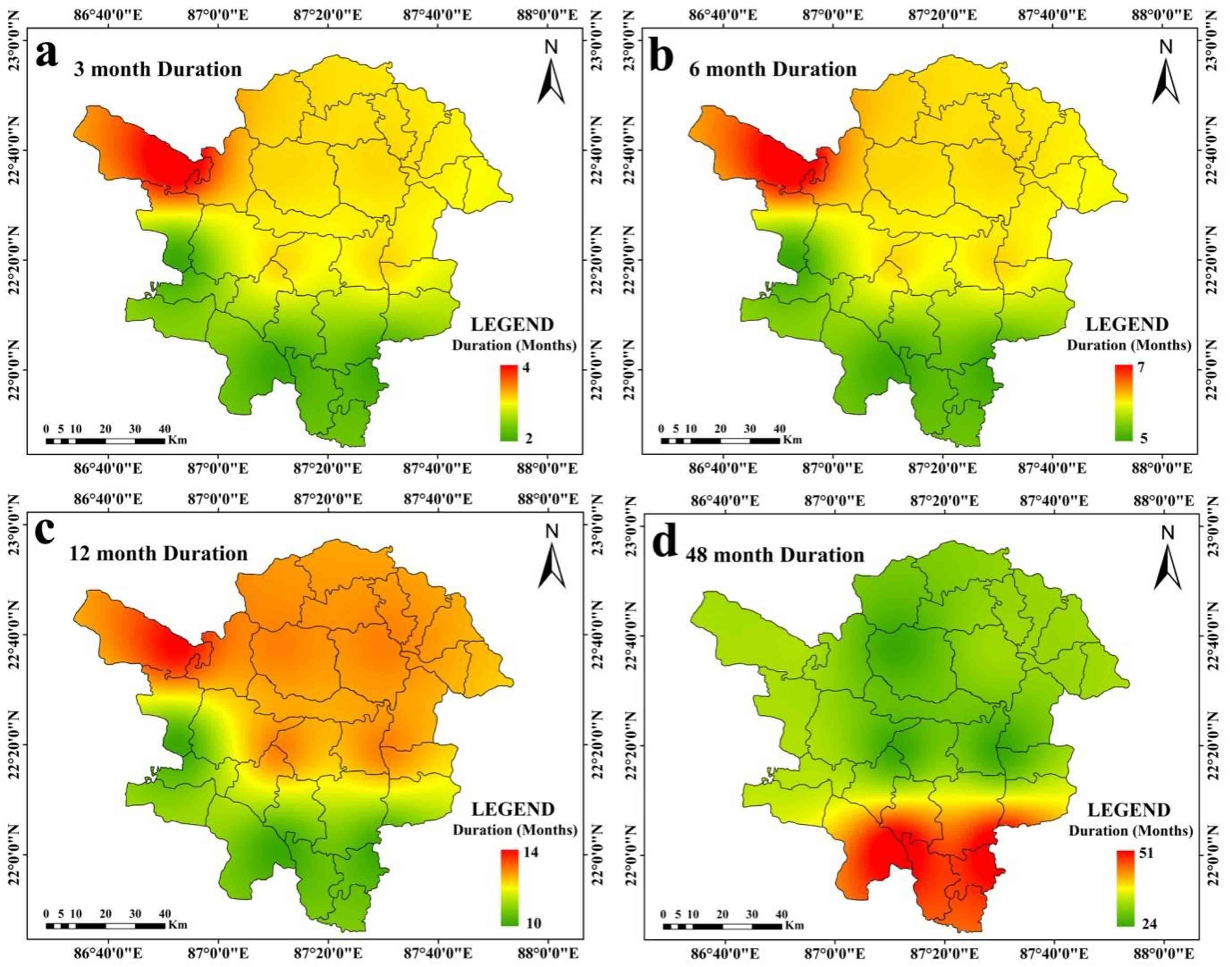
At 48 months’ time step, drought is at the peak, at 220872 (1st Station) and 220875 station (8th Station) with -2.35 SPEI value, which is observed on October 2012 (Table 6). Average drought is also intensified at 220872 (1st Station) and 220875 (8th Station) with -1.49 SPEI value. Drought magnitude is highest at 220872 (1st Station) and 220875 station (8th Station) (-125.63) (Table 7). Average drought duration is also high at 220872 (1st Station) and 220875 station with 14 to 18 months (Figure 6a and Figure 6b). Average drought duration is within 10 to 18 months (Figure 6a-6g). The highest rates of incidence of ES and moderate drought are also seen at stations 220872 (1st Station) and 220875. In the 48 months’ time step, significant negative trend is noticed in 220872 (1st Station), 223872 (2nd Station), 223875 (3rd Station), 226875 (7th Station) and 220875 (8th Station) stations. Other stations are noticed with positive and negative trends of drought which are non-significant in character (Table 6).
Table 6. Station-wise assessment of drought at 48 months
|
Stations
|
Peak intensity (PID)
|
Peak intensity observed
|
Moderate drought occurrence rate
|
Extreme to severe (ES) drought occurrence rate
|
Average intensity
|
Mann-Kendall trend
|
Sen's slope
|
|
220872 (1st Station)
|
-2.35639
|
October-2012
|
18.06
|
14.58
|
-1.49564
|
-0.09*
|
-0.99*
|
|
223872 (2nd Station)
|
-2.21511
|
August-2012
|
6.71
|
2.78
|
-1.44081
|
-0.09*
|
-1.18*
|
|
223875 (3rd Station)
|
-2.21511
|
August-2012
|
6.71
|
2.79
|
-1.44081
|
-0.09*
|
-1.18*
|
|
226869 (4th Station)
|
-1.99327
|
August-2012
|
6.48
|
2.78
|
-1.3773
|
0.03
|
0.07
|
|
223869 (5th Station)
|
-1.99327
|
August-2012
|
6.48
|
2.78
|
-1.3773
|
0.03
|
-0.07
|
|
226872 (6th Station)
|
-2.21511
|
August-2012
|
6.71
|
2.78
|
-1.44081
|
-0.09
|
1.18
|
|
226875 (7th Station)
|
-2.21511
|
August-2012
|
6.71
|
2.79
|
-1.44081
|
-0.09*
|
-1.18*
|
|
220875(8th Station)
|
-2.35639
|
October-2012
|
18.06
|
14.58
|
-1.49564
|
-0.09*
|
-0.99*
|
*At 0.05 significance level.
Table 7. Drought magnitudes
|
Station Code
|
At 3 Months
|
At 6 Months
|
At 12 Months
|
At 48 Months
|
|
220872 (1st Station)
|
-135.96
|
-129.83
|
-138.13
|
-125.63
|
|
223872 (2nd Station)
|
-118.12
|
-119.87
|
-103.37
|
-57.63
|
|
223875 (3rd Station)
|
-118.12
|
-119.87
|
-103.37
|
-57.63
|
|
226869 (4th Station)
|
-113.82
|
-110.84
|
-96.35
|
-48.21
|
|
223869 (5th Station)
|
-113.82
|
-110.84
|
-96.35
|
-48.21
|
|
226872 (6th Station)
|
-118.12
|
-119.87
|
-103.36
|
-57.63
|
|
226875 (7th Station)
|
-118.12
|
-119.87
|
-103.37
|
-57.63
|
|
220875 (8th Station)
|
-135.96
|
-129.84
|
-138.13
|
-125.63
|
*At 0.05 significance level
4.3 Spatial Assessments of Drought
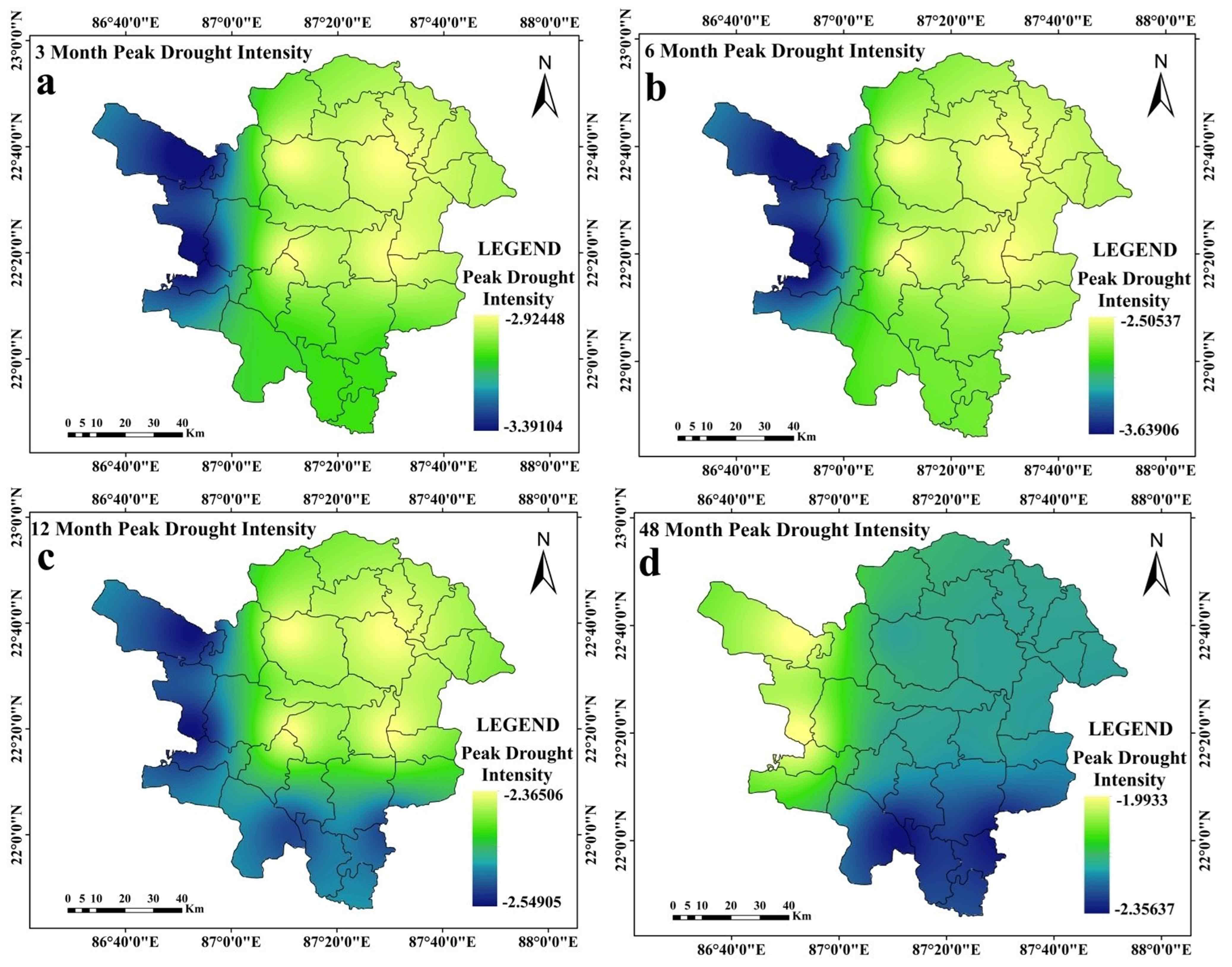
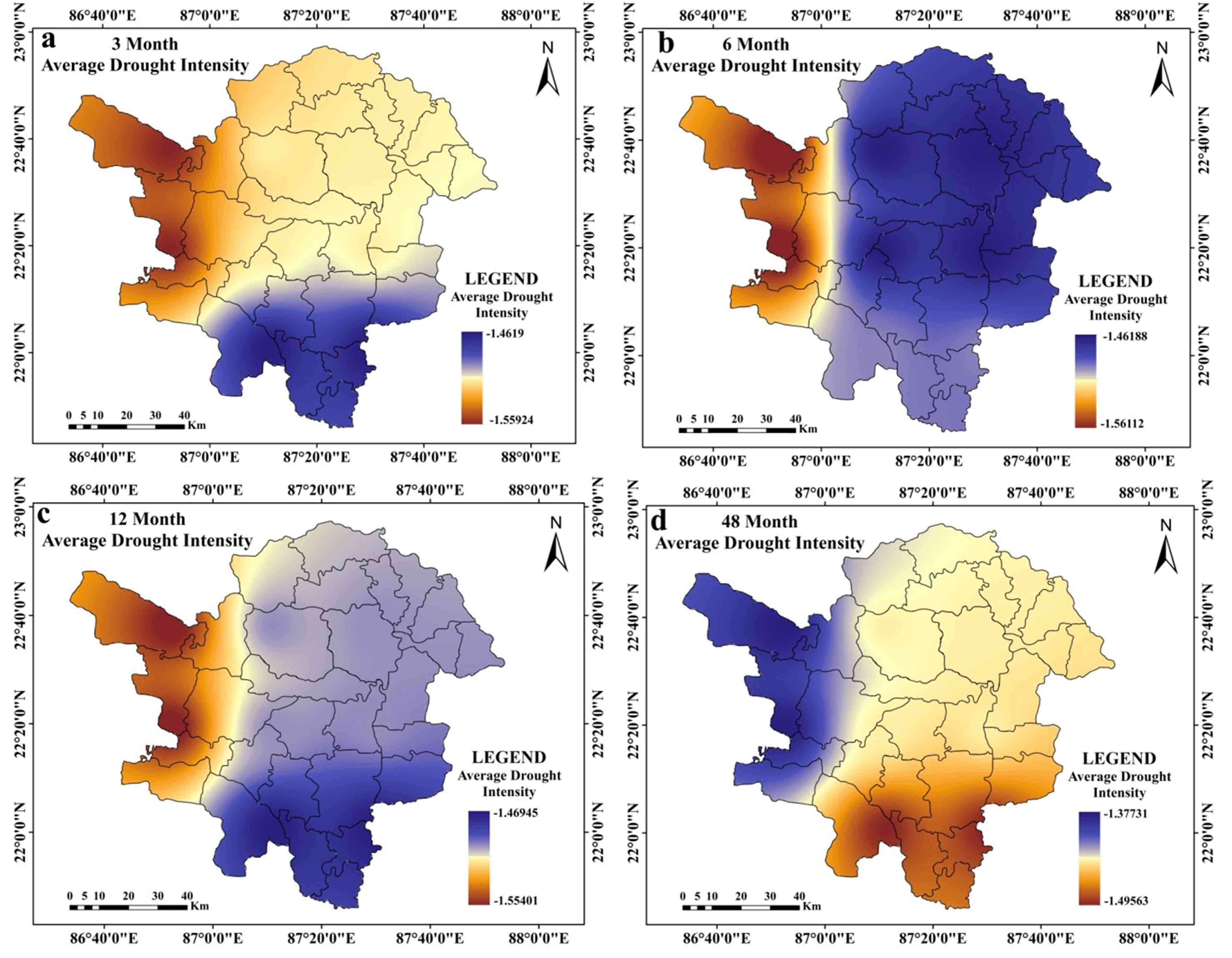
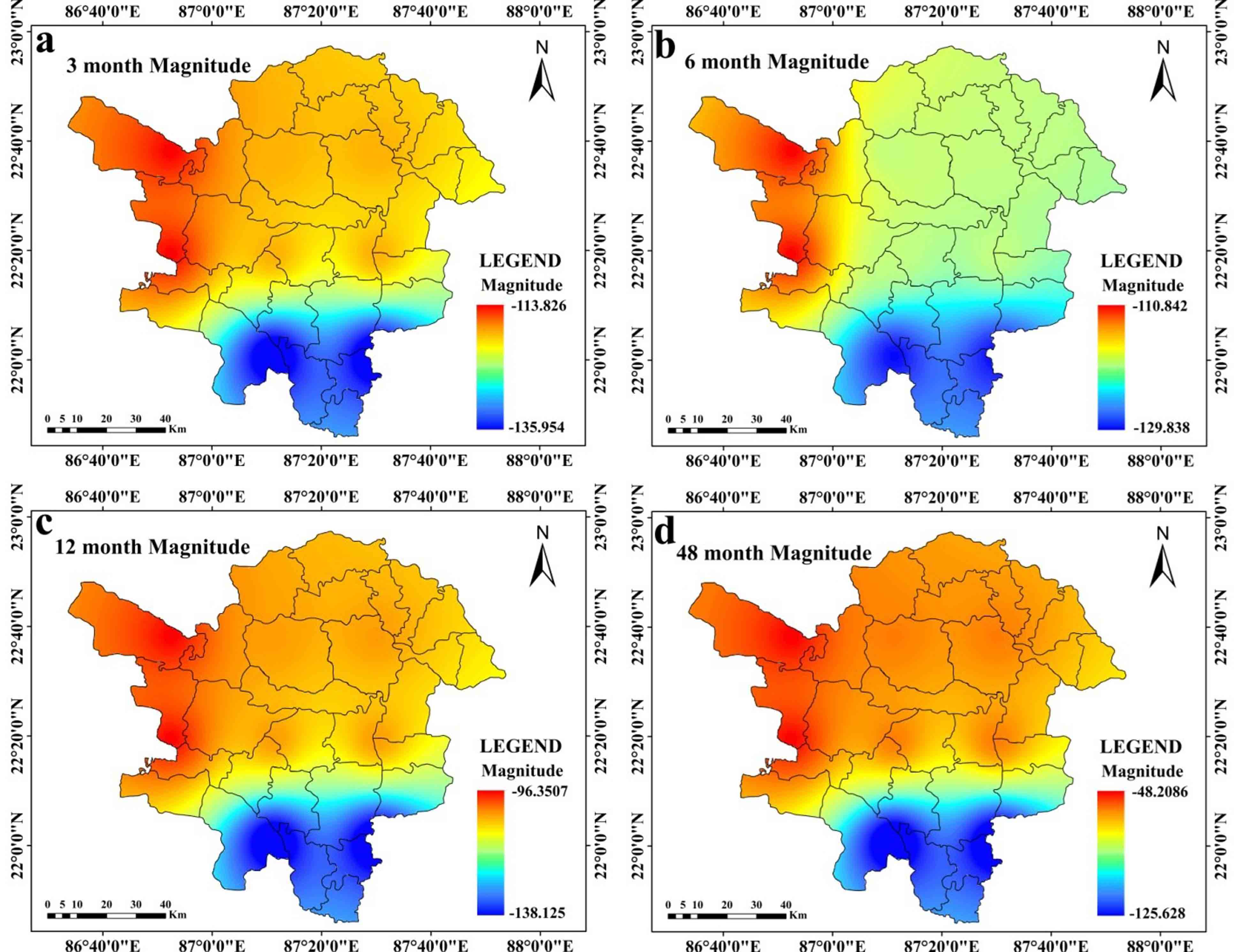
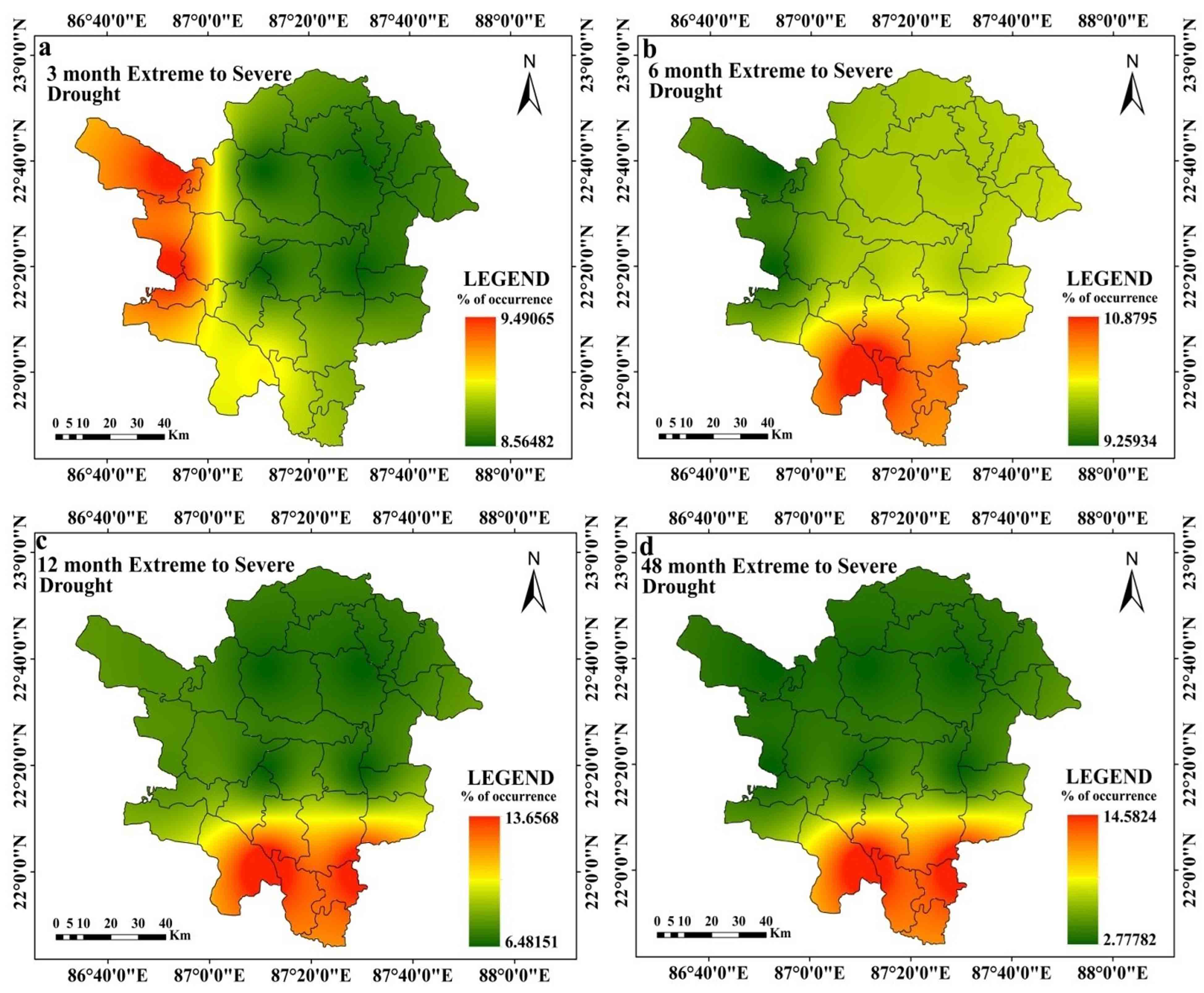
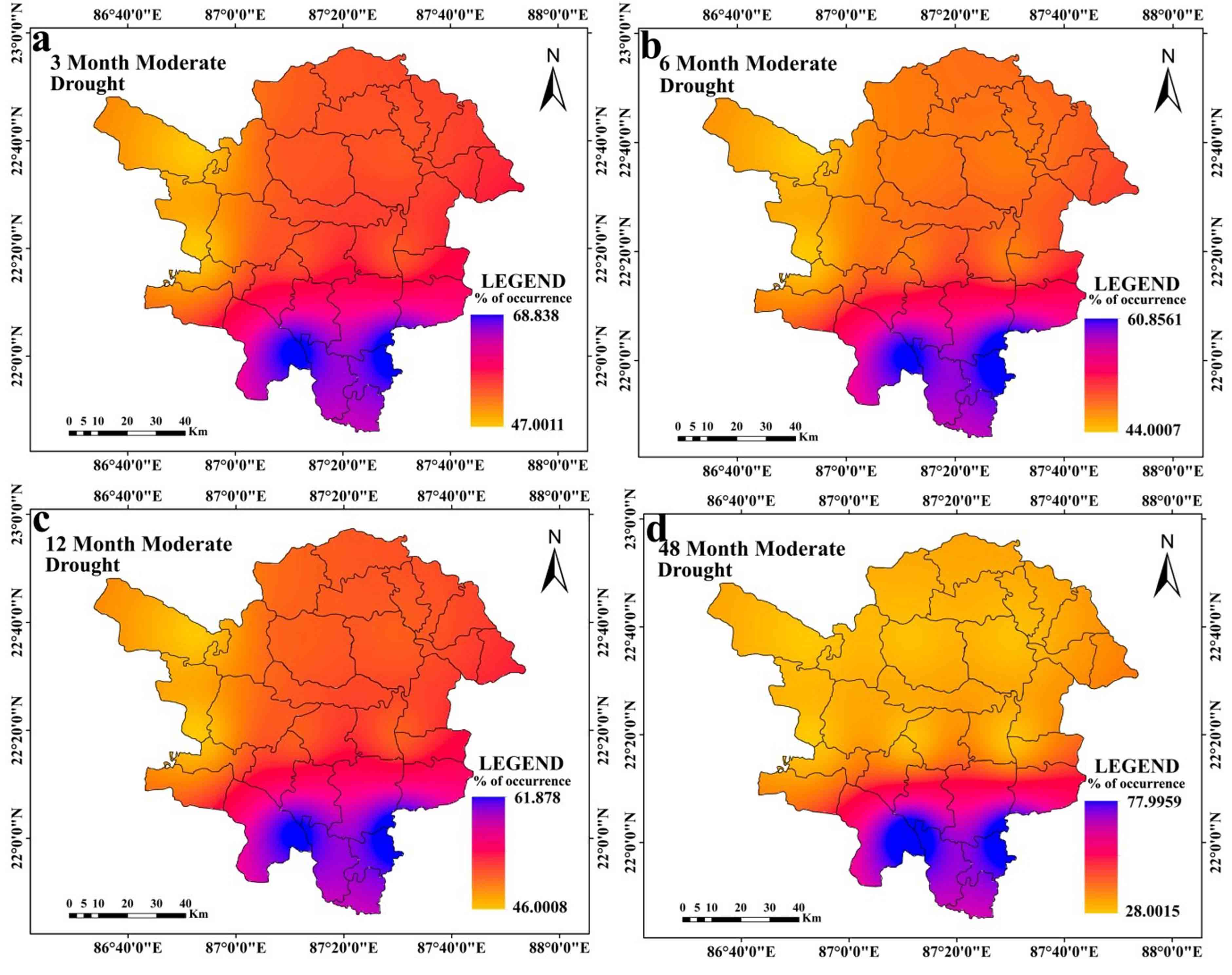
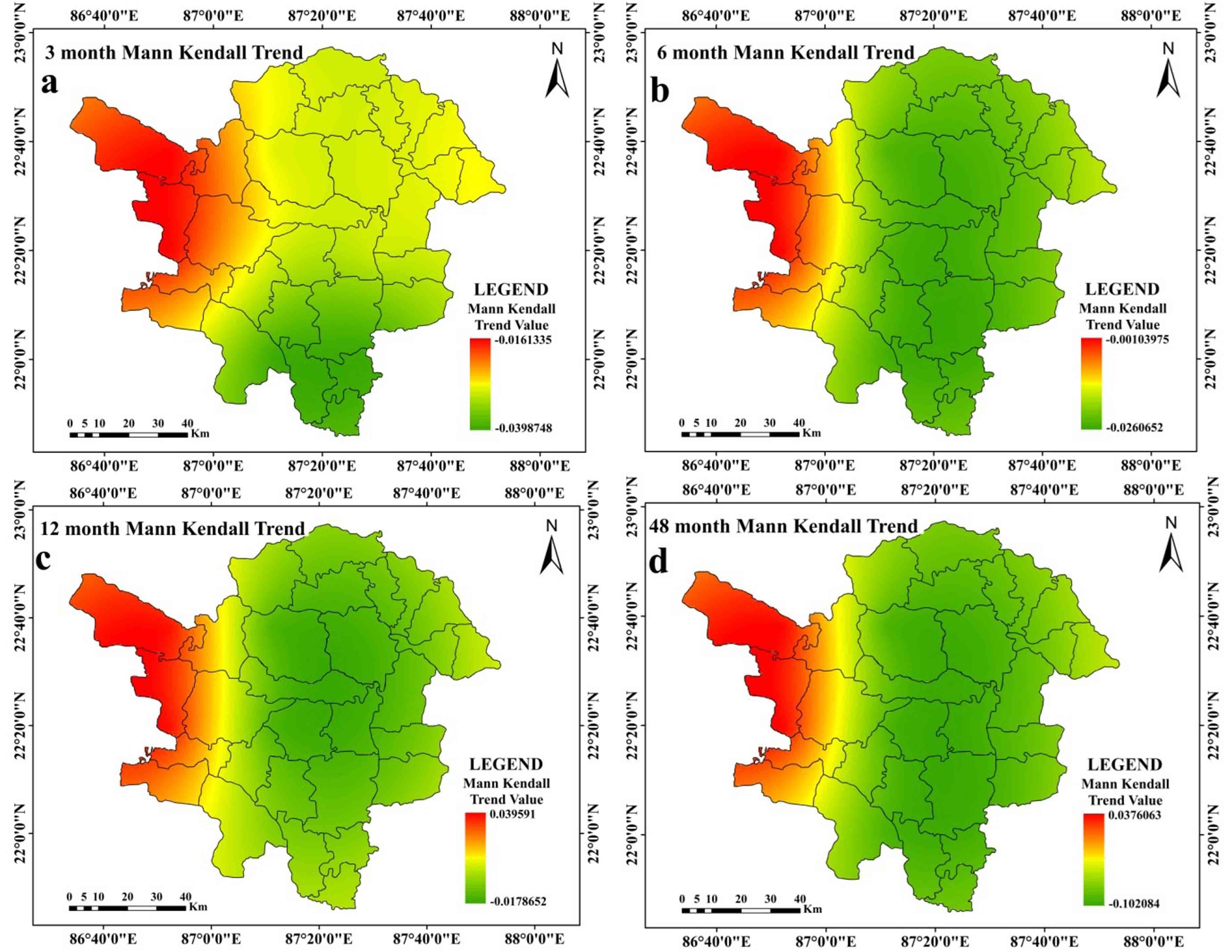
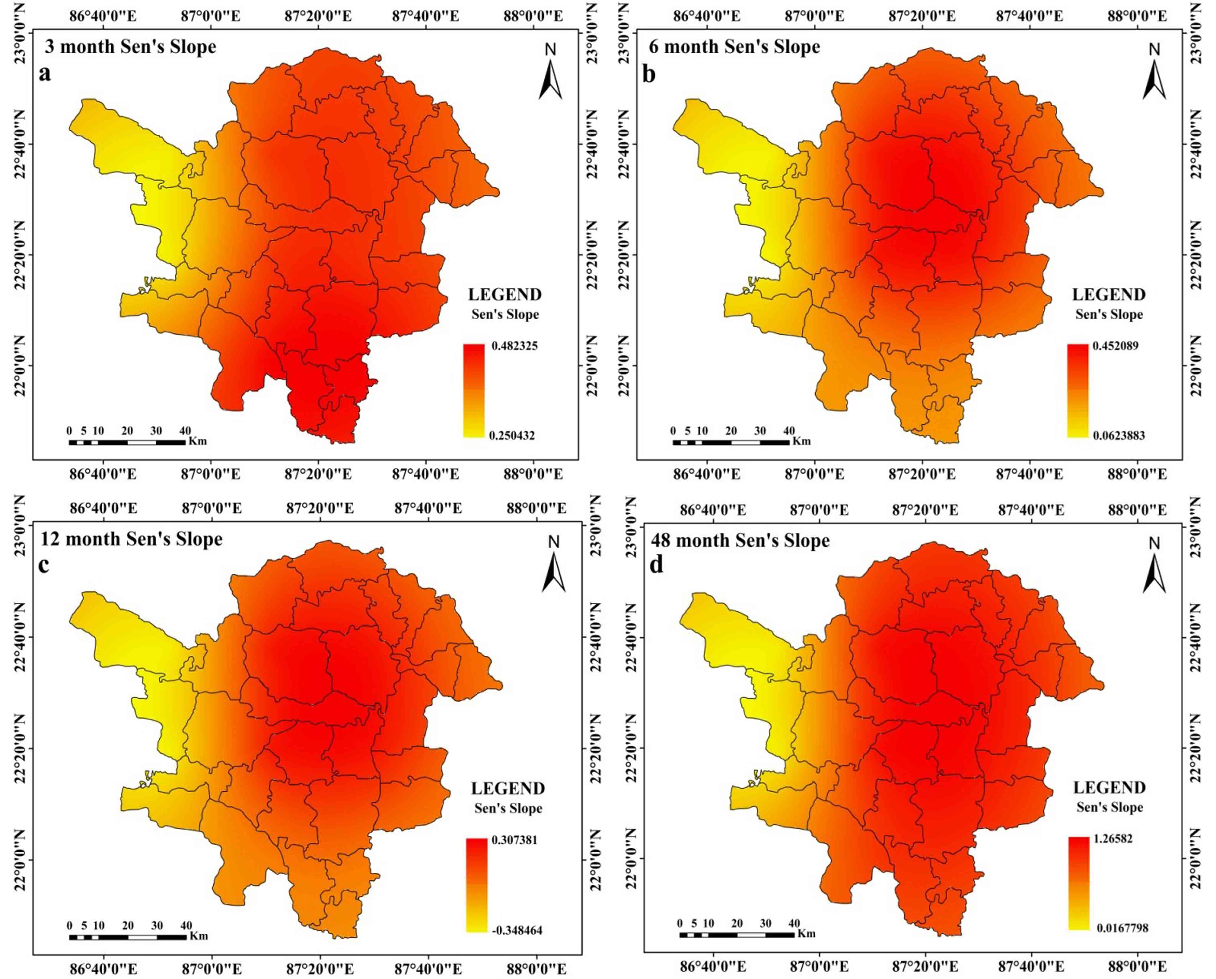
While peak drought is observed in the southern and western portions of the research region at the 12 months time step (Figure 3c), it is at its highest at the 3 months and 6 months time steps in the western portions of the study region. Peak drought moves in the southern parts of the region over a time period of 48 months (Ffigure 3d). At time steps of 3 months, 6 months, and 12 months (Figure 4a, 4b, and 4c, respectively), the average drought in the western parts of the study region gets worse. Southern regions are seen to have greater average drought intensity at a 48-month time step (Figure 4d). Drought is at its’ highest magnitude in southern portions of the study region and this feature is almost similar at all-time steps (Figure 5a-5d). Average drought duration is long in the western parts of the study region for time steps of 3 months, 6 months and 12 months (Figure 6a-6c). Southern regions are seen to have longer average drought durations at 48 months time step (Figure 6d). At 3 months’ time step, western portions of the study area are noticed with highest occurrence rate of ES drought (Figure 7a). At other time steps (6 months, 12 months and 48 months time step) southern portions of the region are noticed with high rate of occurrence of ES drought (Figure 7b, 7c, 7d). At all-time steps, the southern portions are noticed with higher occurrence rate of moderate drought (Figure 8a-8d). At every time steps, negative MK and Sen’s slope value is observed in the western and southwestern portions of the study area (Figure 9a-9d and Figure 10a-10d). Eastern and south-eastern portions are characterized with positive MK and Sen’s slope value (Figure 9a-9d and Figure 10a-10d). The general nature of the region is that as the time step increases, duration of drought starts to increase but intensity, occurrence rate starts to decrease in a significant proportion. Another interesting feature is that drought starts to shift from western portions to southern portions of the study region.
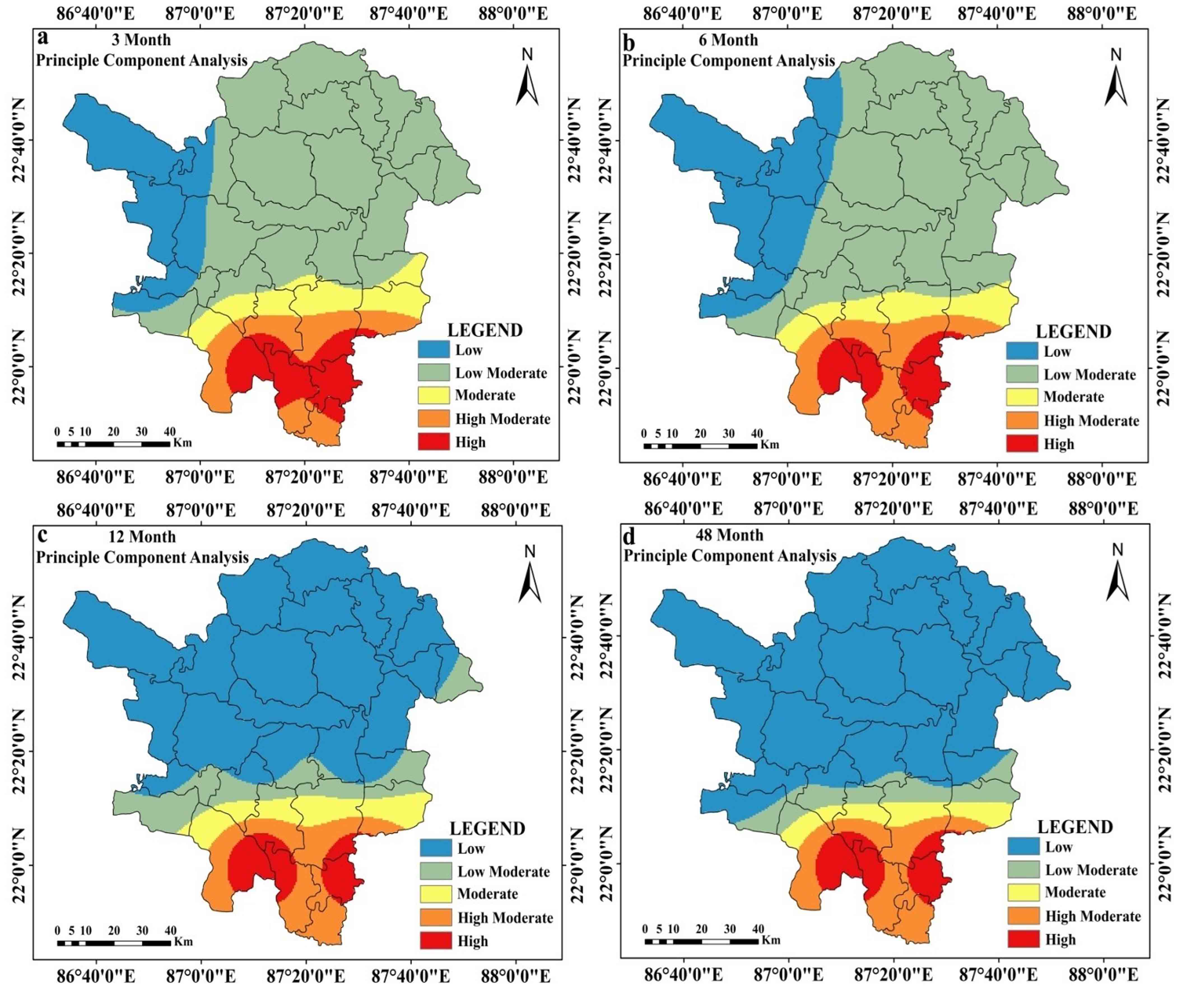
4.4 Assessments of Drought Susceptibility
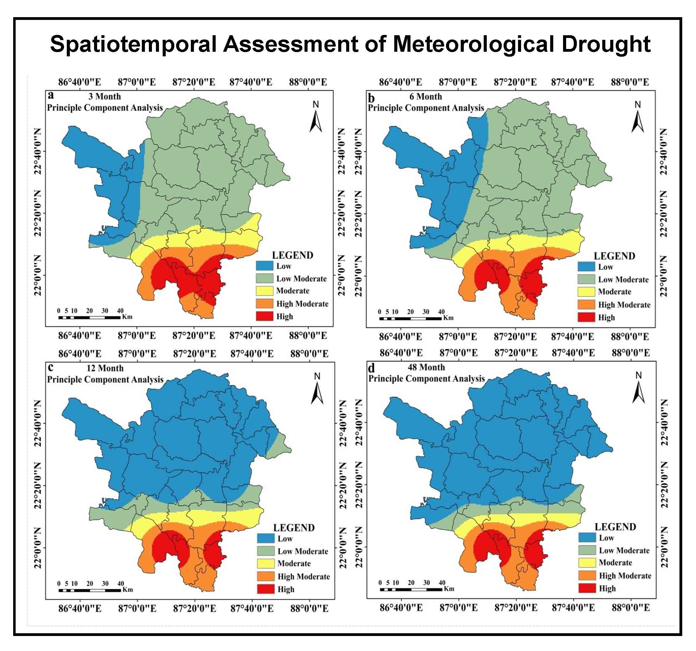
Zones that are susceptible to drought are evaluated using composite PCA scores (PCA). Here, the first four components are utilized because they account for 80% of the total data. Drought is noted as high, high moderate and moderate at the southern regions of at the 3- and 6-months’ time steps. In the eastern and western halves, respectively; the low, moderate and low categories are present (Figure 11a and 11b). High, high moderate, moderate and low moderate categories predominate in the southern regions at the 12- and 48-months time steps. Remaining portions are noticed with the low drought category (Figure 11c and 11d). In aggregate, low and low moderate categories account for 77.32% of the research area. However, 16.03% of the region is classified as high and high moderate. The remaining regions (6.64%) are classified as being in the moderate drought category (Table 8).
Table 8. Estimated area under drought
|
Categories
|
Area (%)
|
|
3 Months
|
6 Months
|
12 Months
|
48 Months
|
Average
|
|
Low
|
16.81
|
22.99
|
66.53
|
72.69
|
44.75
|
|
Low moderate
|
57.36
|
54.02
|
11.42
|
7.50
|
32.57
|
|
Moderate
|
8.41
|
6.71
|
6.65
|
4.79
|
6.64
|
|
High moderate
|
9.17
|
10.13
|
9.80
|
9.27
|
9.59
|
|
High
|
8.26
|
6.16
|
5.60
|
5.75
|
6.44
|


 ,
Sayan Deb 1
,
Sayan Deb 1