Keywords

School Education Quality Index , Panel of experts , India , Education , Composite Education Index

1 . INTRODUCTION

2 . STUDY AREA

Overall, the Madhya Pradesh, Chattisgarh, and Odisha, are considered as the Central Indian states and the Goa, Telangana, Andhra-Pradesh, Karnataka, Maharashtra, Kerala, and Tamil Nadu are considered as the South Indian states in this research (Figure 1).  Climatologically, these sections belong to the hot semi-arid category. Average rainfall and temperature of these portions fluctuate from 400 to 800 millimeter and 20ºC to 24ºC temperature. The post monsoon and early seasons of pre-monsoon is generally drought prone. Madhya Pradesh is located on the border between the Indo-Gangetic Plain to the north and the Deccan plateau to the south. Low hills, broad plateaus, and river valleys define its physiography. Madhya Pradesh’s elevation ranges from 300 to 3900 feets (90 to 1200m). The population growth rate of Madhya Pradesh is 20.35%; and the sex ratio is 931. The child sex ratio of Madhya Pradesh is 918; according to the Census of India, 2011. The state of Chattisgarh experienced 22.61% population growth rate and it had a sex ratio of 991 according to the Census of India, 2011. Average population density of the state was 189 persons/km². Average literacy rate of the state was 70.28%. The state of Odissa had its’ total population of 4.2 crores according to the Census of India, 2011. According to the latest Census data, 14.05% population growth rate was recorded for the Andhra-Pradesh. The average sex ratio of the state was 979 with average literacy rate of 72.87%. According to the Census (2011), approximately 5 crore of population was recorded. The sex ratio of the state was recorded as 993. The population density of the state was recorded as 308. Overall, 67.02% literacy was found for the Andhra Pradesh according to the Census of India, 2011. The Kerala state was marked with 3.34 crores of population, 4.91% population growth rate, the sex ratio of 1084, and about 94.00% sex ratio, according to the District Census Factbook of Kerala (2011). The Tamil Nadu was marked with 7.21 crores of population, 15.61% population growth rate, 996 sex ratio, and 80.09% literacy rate. The Maharastra state was noticed with 11.24 crore population, 15.99% population growth rate, 929 sex ratio, and 82.34% literacy rate according to the Census of India (2011). The Telangana state was found with approximately, 38 crores of population with population density of 800 persons per square km. Overall, literacy rate of the state was 74.83%. 

According to the Budget allocation of 2022; approximately 10,345 crores were allocated by the Madhya Pradesh government for the primary schools, and near about Rs. 6212 crores were allocated for the development of the secondary schools. Near about 32, 843 crores rupees were allocated for the development of this sector (Finance Department Madhya Pradesh, 2022-23). Similarly, the Odissa allocated approximately 3581 crore rupees (Odisha Budget Analysis 2022-23). Near about 1380 crores were allocated for the states of Chattisgarh at the education sector according to the budget plan of 2022-23(Chhattisgarh Budget Analysis 2022-23). During 2022-23, Goa had focused to encourage the higher education and near about, 500 crore rupees were allocated for this purpose. Telangana granted 24% of their budget for their education sector during the financial year of 2022-23(Telangana State Portal Budget Finance, 2022-23). 11.75% of total budget was allocated for the educational sector by the Government of Andhra-Pradesh (Andhra Pradesh Budget Analysis 2021-22). 12% of the total budget was granted by the Karnataka during 2022-23 budget in the higher education (Andhra Pradesh Budget Analysis 2021-22). Near about 28% of the total budget was fixed for the educational sectors of Maharashtra state (Performance Budget, Maharastra, 2022-23). Near about Rs. 2000 crore was fixed by the states of Kerala and Tamil Nadu.

Figure 1. Study area

3 . METHODOLOGY

3.1      Data

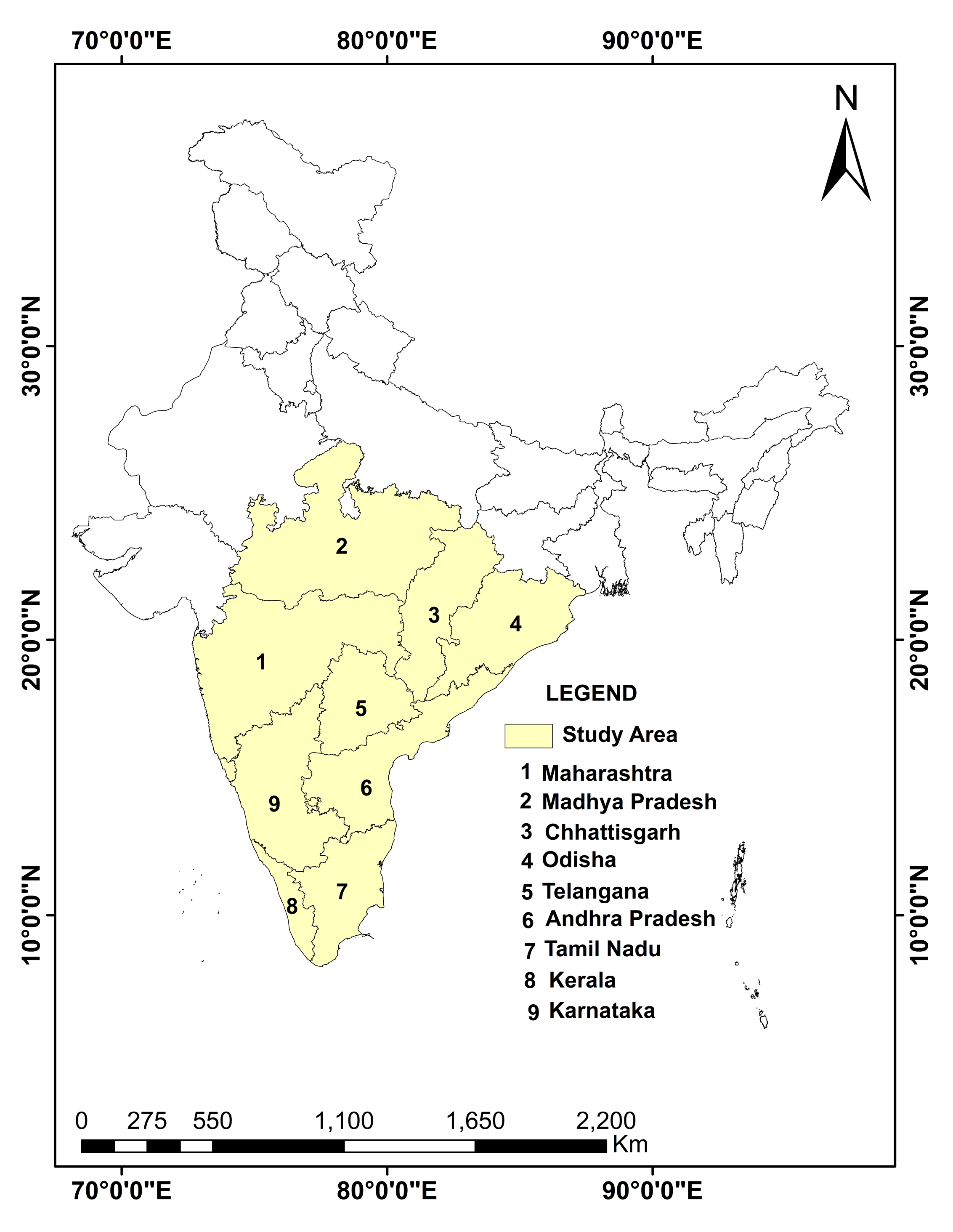
The Gross Enrolment Ratio, Pupil Teacher Ratio, Literacy Rate, Population Density, Population Growth Rate, Density of the Educational Institution, National Highway, and State Highway, Railway, Drinking Water and Toilet Facilities were utilized here, to estimate the Composite Education Index (CEI). The information about the GER (2015-16) and PTR (2015-16) were obtained from the Educational Statistics Databook  (2018). This statistical database was prepared by the collective effort of different institutions under the Ministry of HRD, India to bring the education related data such as, educational attainment, achieved progress through different government schemes etc. The information related to the National and State Highways were collected from the Basic Road Statistics of India (2016-17). Information related to railway (2016-17) was obtained from the Indian Railways Civil Engineering Portal. The datasets of drinking water and toilet facilities (2015-16) were also collected from the Educational Statistics Databook (2018). On the other hand, the datasets of population density, literacy rate, population growth rates were collected from the Census of India (2011). For the purpose of validation, the School Education Quality Index (SEQI) for the base year 2015-16 for the south Indian states was downloaded from the official website of the Niti Ayog (School Education Quality Index, NITI Aayog).

3.2  Analytic Hierarchy Process (AHP)

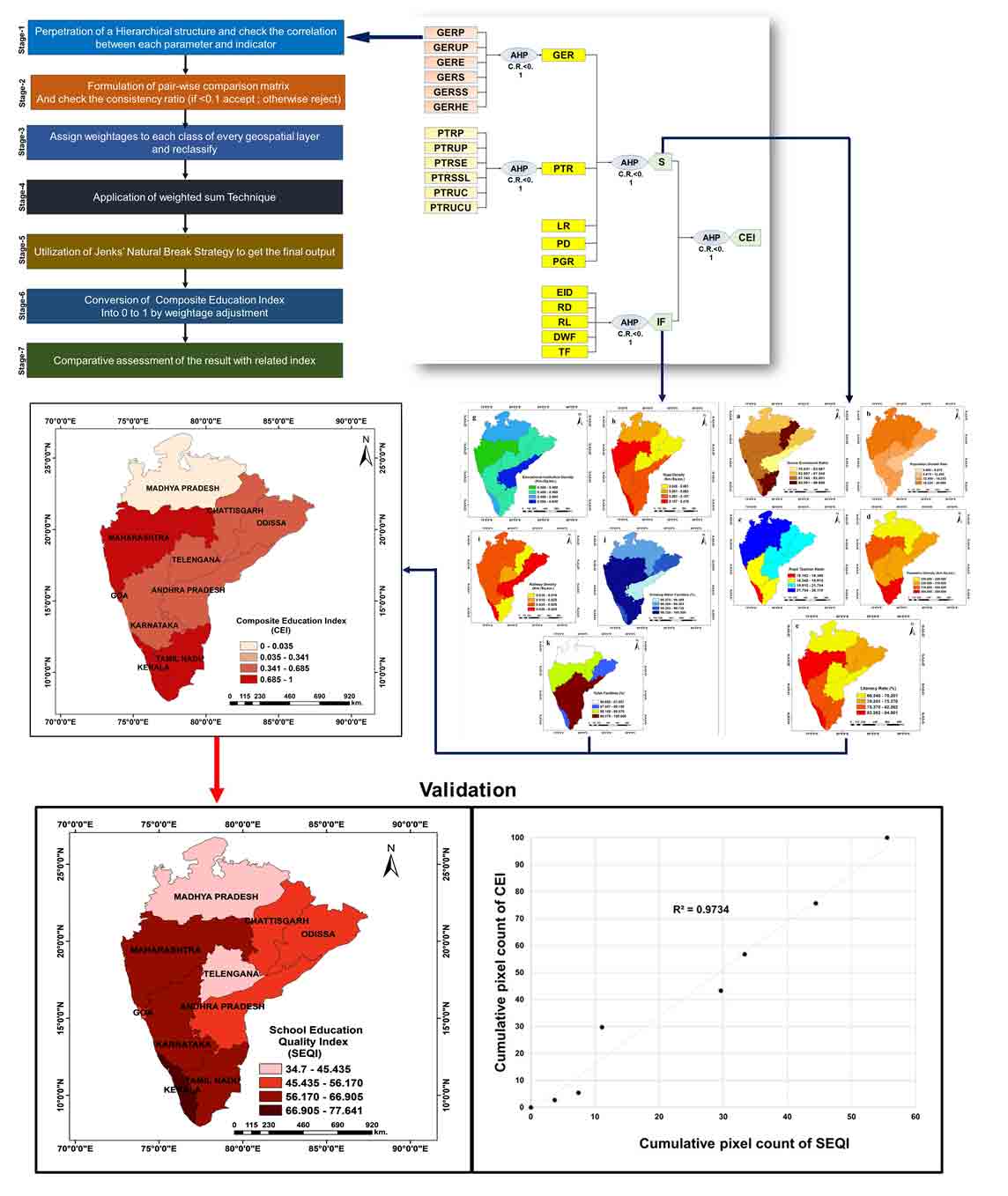
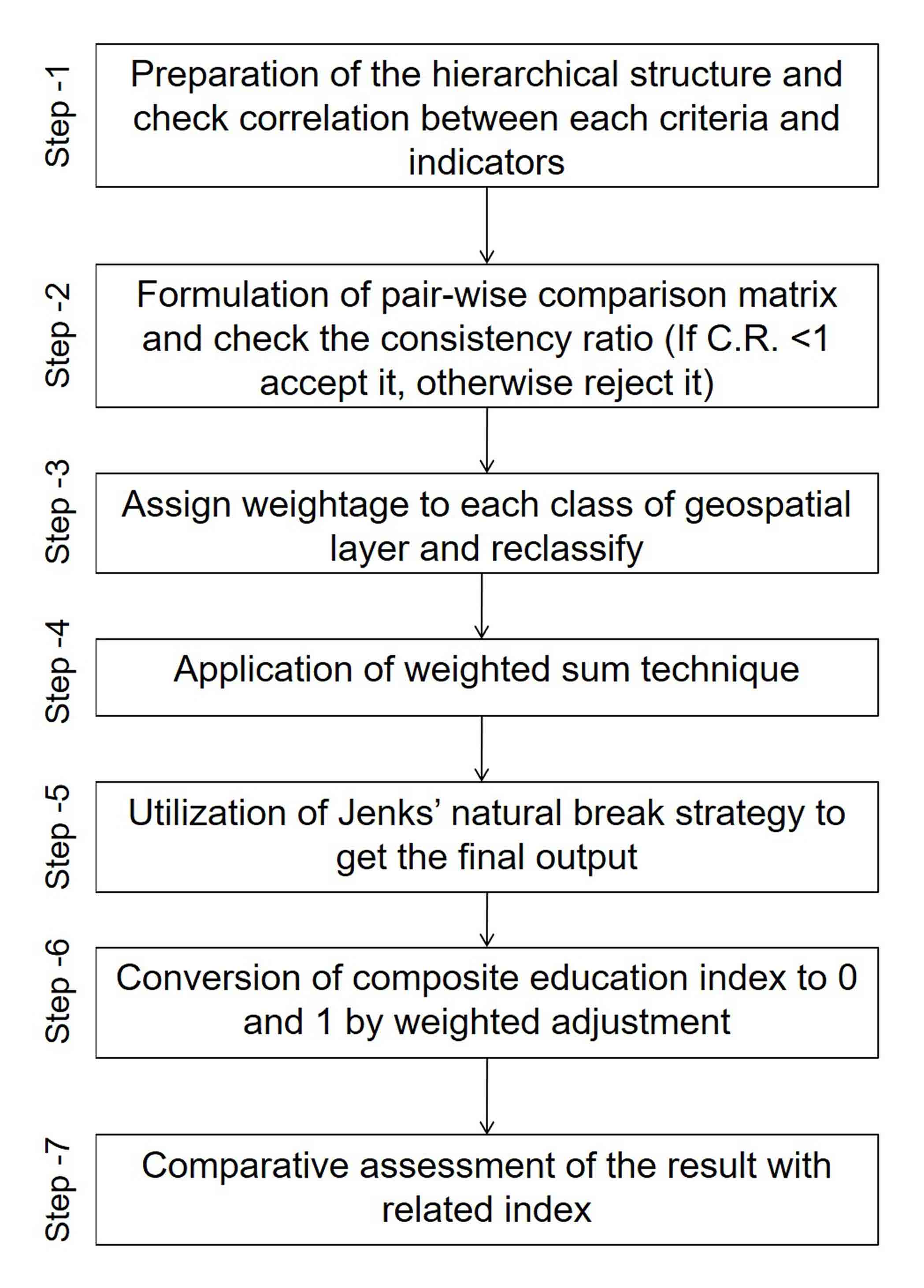
The AHP is an objective MCDM technique to select the best alternative from a wide number of available choices (Kumar et al., 2017; Raha and Gayen, 2022). The AHP method was invented by Saaty, (1987), and it attracted  a wide number of researchers for its’ adaptability and usefulness. Saaty (1987) illustrated the AHP from a strict mathematical ground; which is proved difficult to understand for a novice. The researchers other than the mathematics discipline also find the method very difficult to grasp. Therefore, this research formulated an integrated comprehensive 7 step AHP procedure to formulate the Composite Education Index (CEI) (Figure 2).

Figure 2. Methodology

3.3.1 First step- preparation of a hierarchical structure

The methodology started with the formulation of hierarchical structure, which specified the goal of the complex sub-problem of this research. Here, two parameters, ten criteria and twelve indicators were utilized (Table 1). Those two parameters were from the social and infrastructural perspectives. Ten criteria include the Gross Enrolment Ratio (GER), Pupil Teacher Ratio (PTR), Educational Institution Density (EID), Road Density (RD-National Highway (NH) and State Highway (SH) combined), Railway Density (RL), Facilities of Drinking Water (DWF) and the Toilet Facilities (TF). The GER and TFR both have 6 indicators each, specified into the Table 1. Other criteria have no specific indicators. Gross Enrollment Ratio (GER) is the proportion of all enrolments, irrespective of age, to the population in the age category, that is considered to correspond to the each category of the educational level (Omodero and Nwangwa, 2020; Thapa, 2013). Children receive their first education at primary school, where they learn the fundamentals of reading, writing, and arithmetic as well as the fundamentals of geography, natural science, social science, art, and music (Brophy et al., 2016; DeBoer, 2019). Therefore, their inclusion and enrolment in this sector creates positive ambiences. Similarly, the enrolment of students in the higher education and research are also equally important for a composite overview of an educational sector (Elliott and Shin, 2002; Fafunwa, 2018). Keeping in mind the above fact, the Gross Enrolment Ratio (GER) was considered in this research, which can create positive atmosphere for the learning and teaching. The student-teacher ratio, also known as the student-faculty ratio, measures the proportion of students to teachers at a given school or university (Hoffman, 2014; Snijders et al., 2022). Positive effects like students’ participation and improvement can be nurtured by encouraging interactions between students and the educational teachers and staff (Greenberg et al., 2017; Owen, 2016). When prospective students are choosing postsecondary institutions, a low student-to-teacher ratio is sometimes cited as a selling advantage. On the other hand, a high student-teacher ratio is sometimes used as an argument against comparably overcrowded classrooms or school systems, or as proof that education needs to be given greater financial support (Baird et al., 2017; Newberry and Allsop, 2017). Therefore, GER and PTR are in the positive relationship with educational potentiality and those two criteria were used in this research. The prevalence of educational institutions encourages society’s sustainability (Lozano et al., 2015; Zsóka et al., 2013). It provides chances for pupils, especially those from the remote places and hence, a positive vibration is emerged in the society though the educational institutions (Roberts et al., 2018). Educational institutions create knowledge, wisdom, and awareness, which spread in a particular society spreading a socio-environmental and socioeconomic  balance (Awan, 2021). The natural and social appeal are accurately integrated by the educational institutions, and therefore, the density of the educational institution is an extremely essential factor to be considered in this research (Bansal et al., 2019; Fischer, 2017). Simultaneously, several infrastructural facilities are also required to smooth the educational sectors. The facilities of NH and SH make a smooth overview of the transport facilities; therefore, students and teachers able to reach the educational institutions quite easily (Cole et al., 2010; Lombardi et al., 2012). Therefore, the road and railway density are considered in this research. Similarly, the drinking water and transport facilities help to maintain the sound health and hygiene in the educational institution.

3.2.2 Second step-checking correlation coefficient value and formulation of matrices for pair-wise comparisons

The second step was marked with the preparation of correlation matrices and for each case low correlation coefficient value (<0.8) was obtained (Table 2, Table 3 and Table 4). It proves that each parameter, criteria and indicator is independent, and hardly any mutual relationship exists between each of the pairs. Therefore, those parameters and indicators can be easily be used further, without any doubt. Next the pair-wise comparison matrices were prepared by the equal number of rows and columns, which actually signify the relative importance of each criterion (Chaudhary et al., 2022; Raha and Gayen, 2022). Here, the importance of different parameters, criteria and their indicators were selected by the 10 panel of experts. The panel was created by including those experts and researchers, who had at least five years of experience in the respective field. The preference of each criterion was estimated using a relative dominance scale of 1 to 9 specified in the Table 5 (Saaty, 1987). Here, 1, 3, 5, 7 and 9 were marked as equally important, moderately important, strongly important, very strongly important and extremely important. Further, different literatures were consulted from wider databases like Scopus, Road, Scilit, Garuda, Science Citation Index (Expanded), and Emerging Sources Citation Index (ESCI). Those, scores were further sorted to match the relevance of the educational sector of India. The required steps to formulate the pair-wise comparison matrices are as follows:

1. At first, a pair-wise matrix was developed as follows:

\((X_{ij})_{n\times n}\)  (Table 1)                                      (1)

Where, the criteria are the x and n are the number of criteria.

2. In the second phase, the column wise sum was estimated as follows:

\(X_{ij}=​​\sum^n_i 1X_{ij}\)                                               (2)

3. In the fourth phase, normalized synthesized pair-wise comparison matrices were prepared:

\(X_{ij}=​​ \frac {X_{ij}​​} {\sum^n_i 1X_{ij}}\)                                             (3)

Where, \(X_{ij}\)  is the synthesized matrix.

Therefore, the synthesized matrix can be written as,

\(\begin{bmatrix} X_{11} & X_{12} & X_{13} \\[0.3em] X_{21} & X_{22} & X_{23} \\[0.3em] X_{31} & X_{32} & X_{33} \\[0.3em] \vdots & \vdots & \vdots \end{bmatrix}\)                                   (4)

1. Next, the synthesized matrix was divided by the criteria number (n) to get the weighted matrix or priority vector:

\(W_{ij} = [\frac {\sum^n_i=1X_ij}{n}]\begin{bmatrix} X_{11} \\[0.3em] X_{21} \\[0.3em] X_{31} \\[0.3em] . \\[0.3em] . \\[0.3em] . \\[0.3em] \end{bmatrix}\)                                (5)

Where, \(W_{ij}\)  is the weightages or importance of each selected criterion, which is i. \(X_{ij}\)  is the synthesized matrix.

The consistency ratio was estimated at each phase, which was estimated as follows (Raha and Gayen, 2022; Saaty, 1987):

\(Consistency \ Ratio \ (CR)=​​ \frac {Consistency\ Index \ (C.I.)} {Random \ Index \ (R.I)}\)   (6)

The order of matrix and their corresponding random index value were recorded in the Table 6.

Here, using a relative pair-wise comparison scale of 1 to 9 (Table 5) each of the parameters, criteria and indicators were judged by the ten panel of experts. For example, the primary GER received comparatively higher importance (42.50% weightage), than the other indicators. The GER for the upper primary, secondary, elementary, senior secondary and higher education sectors were marked with respectively, 24.10%, 17.81%, 4.79%, 6.00%, and 4.80% weightages (Table 7). Similarly, the PTR for the upper primary and primary sectors were marked with comparatively higher importance (i.e., 27.90% and 27.30% weightages). PTR for the secondary, senior secondary, university and colleges, and university and constituent units were marked with a comparatively higher priority (i.e., 26.50%, 6.10%, 6.30% and 5.90% weightage, respectively) (Table 8). Again, for the social perspective, the GER and PTR gain comparatively higher importance (i.e., 47.40% weightage, and 26.20% weightage, respectively). On the contrary, the LR, PD and PGR were marked with a comparatively low priority level (i.e., 10.70%, 9.10% and 6.60% respectively) (Table 9). Simultaneously, from the perspectives of the infrastructural facilities (IF), EID was marked with a comparatively higher importance. Other indicators (i.e., RD, RL, DWF and TF) were identified with 26.50%, 10.70%, 7.20% and 4.40% weightages respectively (Table 10). According to Nwogu (2015), two main parameters i.e., social and infrastructural facilities shall be given equal priorities for the determination of effective CEI. Therefore, those two are given equal weightages in this research.

3.2.3 Third step- reclassification of raster layers

In the third stage, each spatial layer and their respective classes were assigned with weightages. Weightages were assigned based on their priority. For each case, increasing or decreasing priority for each geospatial layer was obtained.

At first, the pair-wise comparison matrix ( \(X_{ij}\) ) was multiplied with their corresponding priority or weightage values.

\(\begin{bmatrix} X_{11} & X_{12} & X_{13} \\[0.3em] X_{21} & X_{22} & X_{23} \\[0.3em] X_{31} & X_{32} & X_{33} \\[0.3em] \vdots & \vdots & \vdots \end{bmatrix} \times \begin{bmatrix} W_{13} \\[0.3em] W_{23} \\[0.3em] W_{33} \\[0.3em] \vdots \\[0.3em] \end{bmatrix} = \begin{bmatrix} Xv_{13} \\[0.3em] Xv_{23} \\[0.3em] Xv_{33} \\[0.3em] \vdots \\[0.3em] \end{bmatrix} \)             (7)

Secondly, the resulting cell values were added to get the final raster.

3.2.4 Fourth Step-Application of weighted sum technique

The fourth step was marked by the weighted sum technique, which was implemented here as follows (Raha et al., 2021; Raha and Gayen, 2022):

\(CEI = \sum^n_{i=1} ​​ \sum^q_{k=1} (X_i \times W_k)\)                        (8)

Where, CEI is the Composite Education Index; X_i  is the rank of q thematic layers; W_k  is the weightages of k geospatial layer.

3.2.5 Fifth Step-Application of natural break strategy to get the final output

In the fifth stage, the natural break strategy by Jenk’s were utilized to get the final output. According to Raha and Gayen (2022), the similar values are grouped into the same aggregated class by this method. Therefore, this strategy is fundamental to aggregate the classes.

3.2.6 Sixth step-conversion of CEI into 0 to 1

To make the CEI reproducible, the CEI was adjusted to 0 to 1 in the sixth stage of the methodology. Here, it was adjusted (weighted adjustment) as follows (Raha et al., 2021):

\(CEI_{adjusted} = \frac{CEI_i} {\sum^n_{i} CEI_i} ​\)                                  (9)

As all the considered parameters, criteria and indicators are in positive relationship with educational potentiality, the method of weighted adjustment would be the appropriate one.

3.2.7 Seventh step-validation of CEI with other related index

The seventh stage was marked with the validation of CEI with the SEQI. The School Education Quality Index (SEQI) was created by the NITI Ayog, Govt. of India to assess how well States and Union Territories (UTs) are performing in the field of education. The index seeks to put emphasis on the educational performances by assessing their strengths and shortcomings and make the necessary course corrections or policy interventions. The index aims to make it easier for States and UTs to share knowledge in accordance with NITI Ayog’s mandate in India (Mann, 2022). In this research, the CEI was validated with the SEQI, by assigning the cumulative pixel count of SEQI at the x-axis and the cumulative pixel count of CEI at the y-axis. The Correlation Coefficient (R²) values were utilized to assess the degree of association between two indices.

4 . RESULTS AND DISCUSSION

4.1 Social Parameters

4.1.1 Gross Enrolment Ratio (GER) for the primary level of education

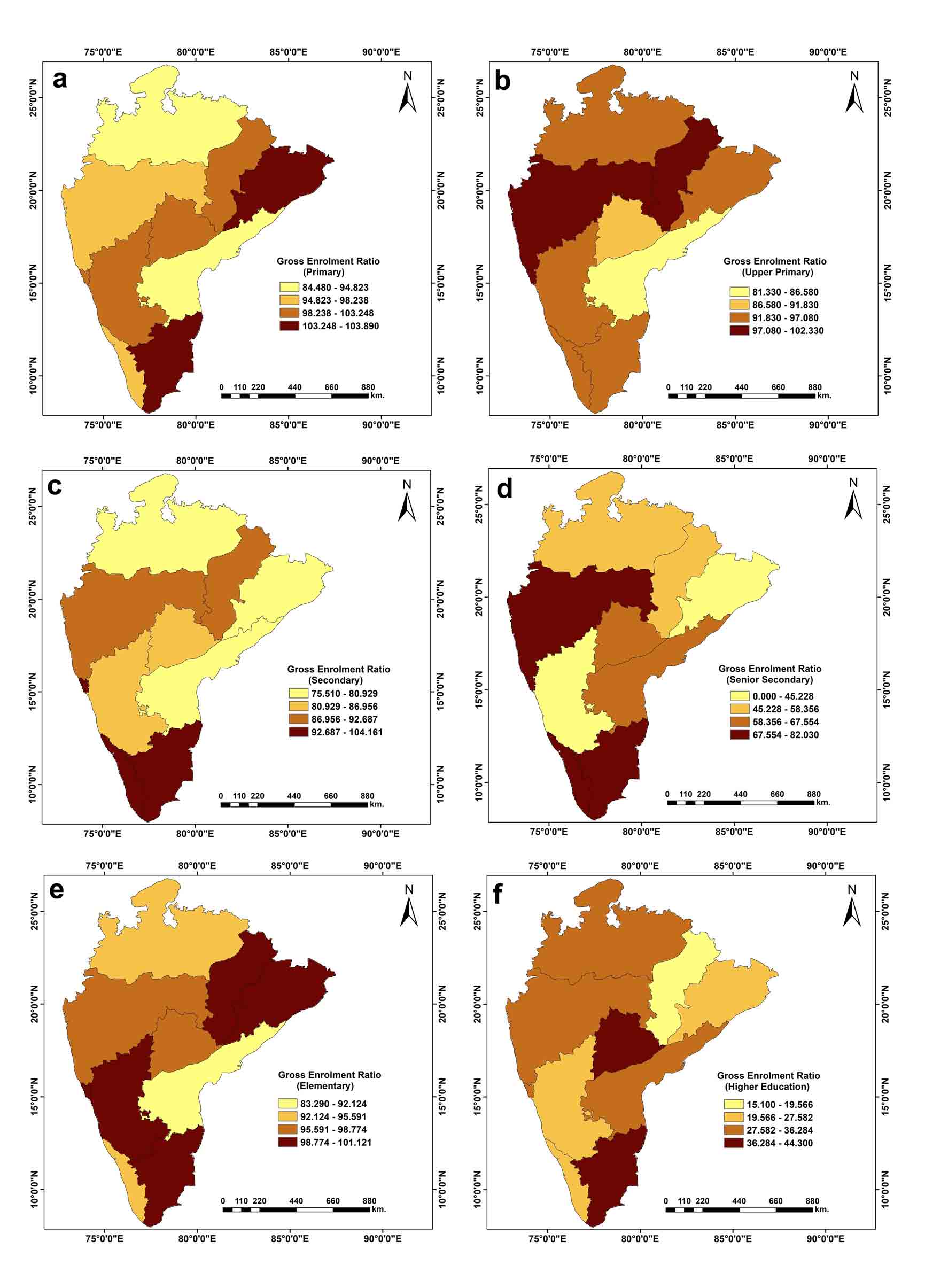
The GER for the primary level of education varied from 84.840 to 103.890. Here, it was classified into 4 groups i.e., 84.489 to 94.823 (31.888% area), 94.823 to 98.238 (22.201% area), 98.238 to 103.248 (27.409% area) and 103.248 to 103.890 (18.503% area). Madhya Pradesh and Tamil Nadu states were found with a very low GER (84.489 to 94.823) (Figure 3a). Maharashtra and Kerala states were marked with a comparatively low GER (i.e. 94.823 to 98.238). Chhattisgarh, Telangana, Karnataka and Goa were identified with a high GER (98.238 to 103.248 GER). Remaining states (Odisha and Tamil Nadu) were identified with 103.248 to 103.890 GER. GER at the primary level positively influences the potentiality of education. Therefore, as the class value of GER increases, priority also increases. All relevant classes were coded as 1, 5, 7 and 9, respectively, with increasing priorities (Table 11).

Figure 3. GER: a) Primary b) Upper-primary c) Secondary d) Senior-secondary e) Elementary and f) Higher-education

4.1.2 Gross Enrolment Ratio (GER) for the upper primary level of education

The GER fluctuated from 81.330 to 102.330 for the upper-primary level. Here, it was categorized into 4 classes i.e., very low GER (81.330 to 86.580) (11.176% area), low GER (86.580 to 91.830) (6.582% area), high GER (91.830 to 97.080) (53.860% area) and very high GER (97.080 to 102.330) (28.381% area).Very low GER (81.330 to 91.830 GER) was observed for only Andhra Pradesh and Telangana states. Remaining states (i.e., Madhya Pradesh, Odisha, Maharashtra, Chhattisgarh, Karnataka, Kerala and Tamil Nadu states) were observed with 91.830 to 102.330 GER (for the upper primary level of education) (Figure 3b). The potentiality of education at the upper primary level is favorably vibrated by GER. By following this recommendation here, as the class value of GER increases, priority increases (i.e., 1, 4, 6 and 8 respectively) and vice-versa (Table 11).

4.1.3 Gross Enrolment Ratio (GER) for the secondary level of education

The GER for the secondary level of education fluctuated from 75.510 to 104.161. It was grouped into 4 classes, i.e., very low GER (75.510 to 80.929) (41.994% area), low GER (80.929 to 86.956) (18.768% area), high GER (86.956 to 92.687) (28.174% area) and very high GER (92.687 to 104.161) (11.064% area). Madhya Pradesh, Odisha, Andhra Pradesh, Telangana and Karnataka states were noticed with a very low GER (75.510 to 86.956 GER) for the secondary level (Figure 3c). The remaining states were observed with 86.956 to 104.161 GER (for secondary level). GER for secondary level is in a positive association with the educational potentiality. So, as the GER for secondary level flourishes, the educational potentiality also flourishes and vice-versa. Following the above proposition, here, all classes of education were coded with 1, 4, 7 and 9, respectively (Table 11).

4.1.4 Gross Enrolment Ratio (GER) for the senior-secondary level of education

The GER for senior secondary level of education ranged from 0 to 82.030. Odisha, Karnataka, Telangana and Andhra Pradesh were noticed with 0.000 to 58.356 GER for the senior-secondary level of education. Kerala, Tamil Nadu, Goa, Maharashtra, Telangana and Andhra Pradesh were marked with 58.356 to 82.030 GER (senior-secondary level of education) (Figure 3d). GER for senior-secondary level of education was categorized into 4 groups, i.e., very low GER (0.000 to 45.228) (22.292% area), low GER (45.228 to 58.356) (29.145% area), high GER (58.356 to 67.554) (17.758% area), and very high GER (67.554 to 82.030) (30.805% area) and those were recoded with 1, 4, 6 and 9, respectively. GER for senior secondary level was positively associated with the potentiality of education (Table 11).

4.1.5 Gross Enrolment Ratio (GER) for the elementary level of education

The Gross Enrolment Ratio (GER) for the elementary level of education fluctuated from 83.290 to 101.121. Andhra Pradesh was observed with a comparatively low GER at the elementary level (83.290 to 92.124).  Kerala, Madhya Pradesh, Maharashtra and Telangana states were marked with a low GER (92.124 to 98.774) at the elementary level. Chhattisgarh, Goa, Karnataka, Odisha and Tamil Nadu were noticed with a very high GER (98.774 to 101.121 GER) at the elementary level (Figure 3e). Here, GER was grouped into 4 classes and those classes were reclassified with 1 (5.8% area), 3 (14.5% area), 5 (37.7% area) and 9 (42.0% area), respectively.  As the GER at the elementary level increases, the potentiality of the education also flourishes and vice-versa (Table 11).

4.1.6 Gross Enrolment Ratio (GER) for the higher education

For higher education, GER varies from 15.100 to 44.300. Here, Chhattisgarh is observed with the lowest GER for higher education. Telangana and Tamil Nadu were marked with the highest GER for higher education. Remaining states were noticed with 19.566 to 36.284 GER (for higher education) (Figure 3f). The GER for higher education was classified here into 4 groups i.e., very low GER (15.100 to 19.566) (8.433% area), low GER (19.566 to 27.582) (24.752% area), high GER (27.582 to 36.284) (51.836% area) and very high GER (36.284 to 44.300) (14.979% area). The GER (for higher education) was positively linked to the educational potentiality. It is clear that as the Gross Enrolment Ratio increases the priority also increases. More importantly, higher GER values are assigned with the higher priority. Therefore the highlighted line should be modified as “Higher GER values are assigned with higher priority”. (Table 11).

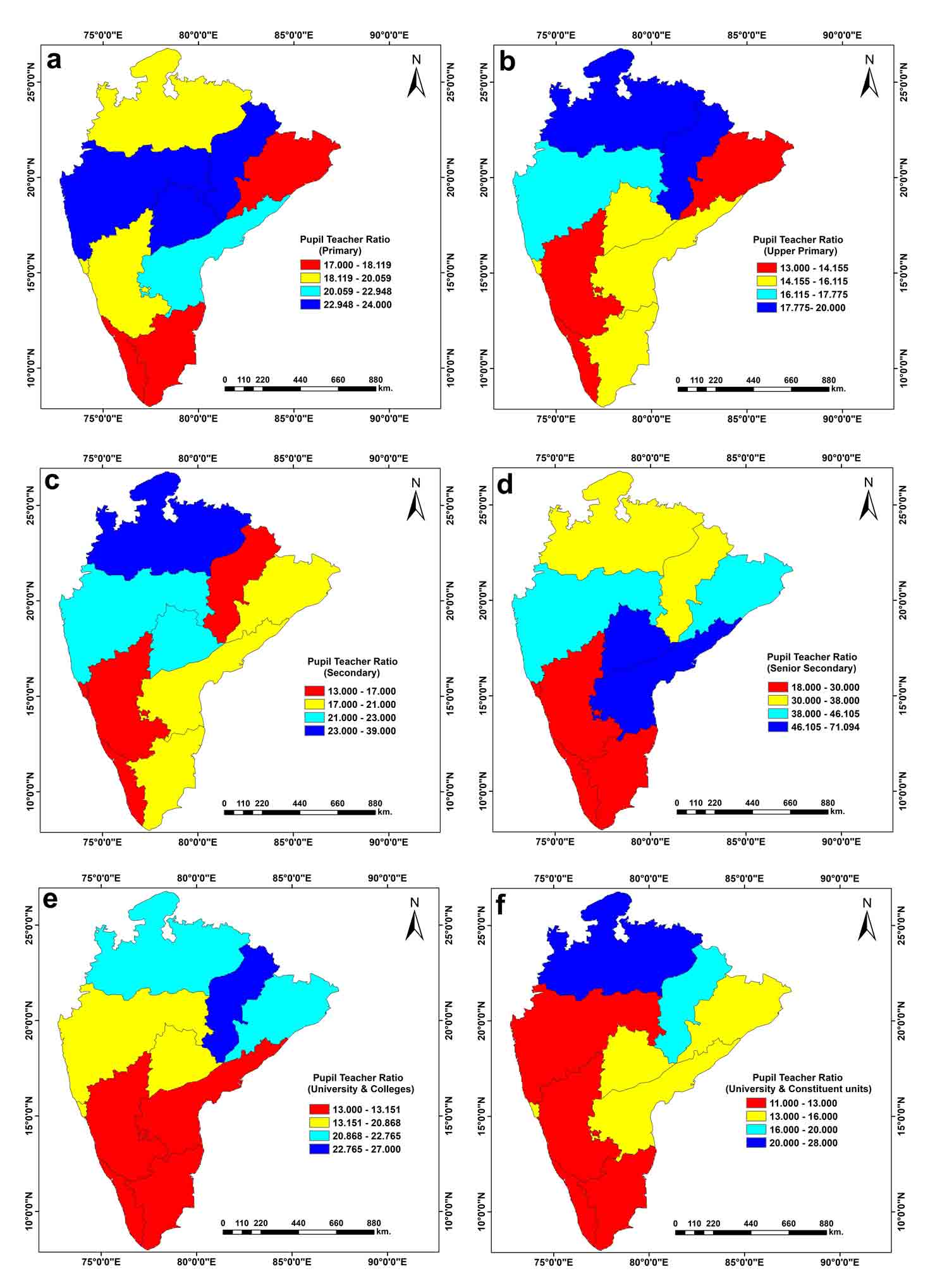
4.1.7 Pupil Teacher Ratio (PTR) for the primary level of education

For the primary level of education, PTR varied from 17.000 to 24.000. For the primary level, Odisha, Kerala and Tamil Nadu were marked with a relatively low PTR (17.000 to 18.119). Madhya Pradesh, Goa and Karnataka were noticed with 18.119 to 20.059 PTR values. Maharashtra, Telangana and Chhattisgarh were marked with relatively high PTR value at the primary level (22.948 to 24.000). The remaining states were observed with a 20.059 to 22.948 PTR value (Figure 4a). PTR at the primary level is favorably connected with the potentiality of education. Therefore, as the PTR increases, the potentiality also flourishes and vice-versa. Following this assumption, the PTR at the primary level is reclassified into 4 groups and they are recoded with 1 (20.963% area), 3 (33.104% area), 5 (11.176% area) and 7 (34.756% area), respectively (Table 11).

Figure 4. PTR: a) Primary b) Upper-primary c) Secondary d) Senior-secondary e) University and Colleges f) University and constituent units

4.1.8 Pupil Teacher Ratio (PTR) for the upper primary level of education

PTR for the upper primary level fluctuated from 13.000 to 20.000. Madhya Pradesh and Chhattisgarh states had the highest PTR (17.775 to 20.000) at the upper-primary level. On the contrary, Odisha, Karnataka and Kerala states had the lowest Pupil Teacher Ratio (PTR). The remaining states (i.e., Maharashtra, Telangana, Goa, Andhra Pradesh and Tamil Nadu) were noticed with 14.155 to 17.775 PTR values (Figure 4b). The PTR at the upper-primary level was categorized into 4 classes, i.e., 13.000 to 14.155 (24.752% area), 14.155 to 16.115 (26.362% area), 16.115 to 17.775 (19.741% area) and 17.775 to 20.000 (29.145% area). The potential of education is positively oscillated with the increasing nature of the Pupil Teacher Ratio (PTR). Following the above recommendation, PTR was reclassified into 4 groups and those were recoded as 1, 5, 7 and 9 weightages, respectively (Table 11).

4.1.9 Pupil Teacher Ratio (PTR) for the secondary level of education

For the secondary level, PTR varied from 13.000 to 39.000. Chhattisgarh, Goa, Karnataka and Kerala had relatively low PTR values (13.000 to 17.000). On the other hand, Madhya Pradesh had a comparatively high PTR value (23.000 to 39.000) for the secondary level. The remaining states (i.e., Odisha, Andhra Pradesh, Tamil Nadu, Maharashtra and Telangana states) were identified with 17.000 to 23.000 PTRs for the secondary level (Figure 4c). The PTR for the secondary level had a positive favorable connection with the potentiality of education. Here, the PTR was regrouped into 4 classes. Following the above recommendation, the classes as mentioned earlier were recoded with 1 (23.286% area), 5 (29.680% area), 7(26.323% area) and 9 (20.711% area), respectively (Table 11).

4.1.10 Pupil Teacher Ratio (PTR) for the senior-secondary level of education

The PTR for the senior secondary level ranged from 18.000 to 71.094. For the senior secondary level, relatively low PTR (18.000 to 30.000) was found for Goa, Karnataka, Kerala and Tamil Nadu states. Relatively high PTR (38.000 to 71.094) was found for Maharashtra, Odisha, Telangana and Andhra-Pradesh states. PTR is positively linked with the potential status of education (Figure 4d). For the senior-secondary level, the PTR is grouped into 4 classes, i.e., very low PTR (18.000 to 30.000) (23.250% area), low PTR (30.000 to 38.000) (29.145% area), high PTR (38.000 to 46.105) (29.847% area) and very high PTR (46.105 to 71.094) (17.758% area). Following the above recommendation, later those were reclassified into 4 groups, i.e., 2, 5, 6 and 7, respectively. As the PTR increases, priority also increases and vice-versa (Table 11).

4.1.11 Pupil Teacher Ratio (PTR) for university and colleges

The PTR for the university and colleges ranged from 13.000 to 27.000. A low pupil-teacher ratio (13.000 to 13.151) for universities and colleges was found for Maharashtra, Andhra Pradesh, Kerala and Tamil Nadu states. On the contrary, relatively high PTR values were noticed for Madhya Pradesh, Odisha and Chhattisgarh states. The remaining (Maharashtra and Telangana) states have 13.151 to 20.868 PTR values (Figure 4e). PTR for universities and colleges is positively associated with the potentiality of education. Following this proposition, here, the PTR was reclassified with 2 (34.219% area), 4 (26.530% area), 7 (39.818% area) and 9 (8.433% area), respectively. Priority increases with an increasing class value and vice-versa (Table 11).

4.1.12 Pupil Teacher Ratio (PTR) for university and constituent units

For university and constituent units, PTR fluctuated from 11.00 to 28.00. Apart from the Madhya Pradesh and Chhattisgarh states, all states had a comparatively low PTR value (11.00 to 13.00) (Figure 4f). PTR here is positively linked with the potentiality of education and therefore, here, the reclassified raster layers were recoded with 1 (42.78% area), 4 (28.07% area), 7 (8.43% area) and 9 (20.71% area), respectively with increasing class values. As the PTR increases, the potentiality flourishes and vice-versa (Table 11).

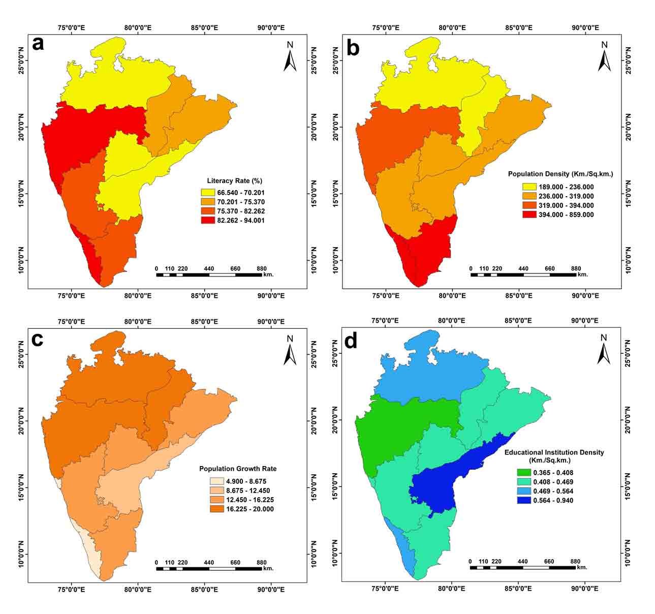
4.1.13  Literacy rate

Literacy rates of the study area varied from 66.540 to 94.001. Madhya Pradesh, Telangana and Andhra Pradesh states were noticed with comparatively low literacy rate (66.54 % to 70.20 %). Maharashtra, Goa, Tamil Nadu, Kerala and Karnataka states were marked with 75.370% literacy rate to 94.001% literacy rate (Figure 5a). Literacy rate positively influences the potentiality of education. Here, literacy rate (%) was classified into 4 classes i.e., very low LR (66.54% to 70.20%) (38.47% area), low LR (70.20% to 75.370%) (18.54% area), high LR (76.37% to 82.26%) (20.58% area) and very high LR (82.26% to 94.001%) (22.40% area) and following the above recommendation, those classes are recoded with 1, 3, 5 and 9, respectively with increasing class values (Table 11).

4.1.14 Population density

Relatively high population densities (319 persons/km² to 859 persons/km²) were found in Maharashtra, Goa, Kerala and Tamil Nadu states. On the other hand, relatively low population densities (189 persons/km² to 319 persons/km²) were marked in Madhya Pradesh, Chhattisgarh, Karnataka, Andhra Pradesh, Telangana and Odisha states (Figure 5b). Here, population densities were classified into 4 classes i.e., very high density (189.000 to 236.000) (19.856% area), high density (236.000 to 319.000) (19.948% area), low density (319.000 to 394.000) (40.051% area) and very low density (394.000 to 859.000) (29.145% area). Low population densities were positively and favorably associated with the potentiality of education. Therefore, here, as population densities increase, priority decreases and vice versa. All the above classes are recoded as 6, 5, 4 and 3, respectively (Table 11).

Figure 5. Other social criteria: a) Literacy Rate b) Population density c) Population Growth Rate d) Density of educational institutions

4.2 Infrastructural Facilities

4.2.1 Densities of educational institutions

Densities for educational institutions varied from 0.365 to 0.940. Maharashtra, Goa, Karnataka, Telangana, Tamil Nadu, Chhattisgarh and Odisha states were marked with relatively low institutional density value (0.365 to 0.469). On the contrary, Madhya Pradesh, Kerala and Andhra Pradesh states were marked with relatively high density (0.469 to 0.940) (Figure 5d). The density of the educational institutions positively influences the potentiality of education. Therefore, all classes were recoded with 1 (30.917% area), 2 (45.912% area) and 3 (23.171% area), respectively, with increasing densities.

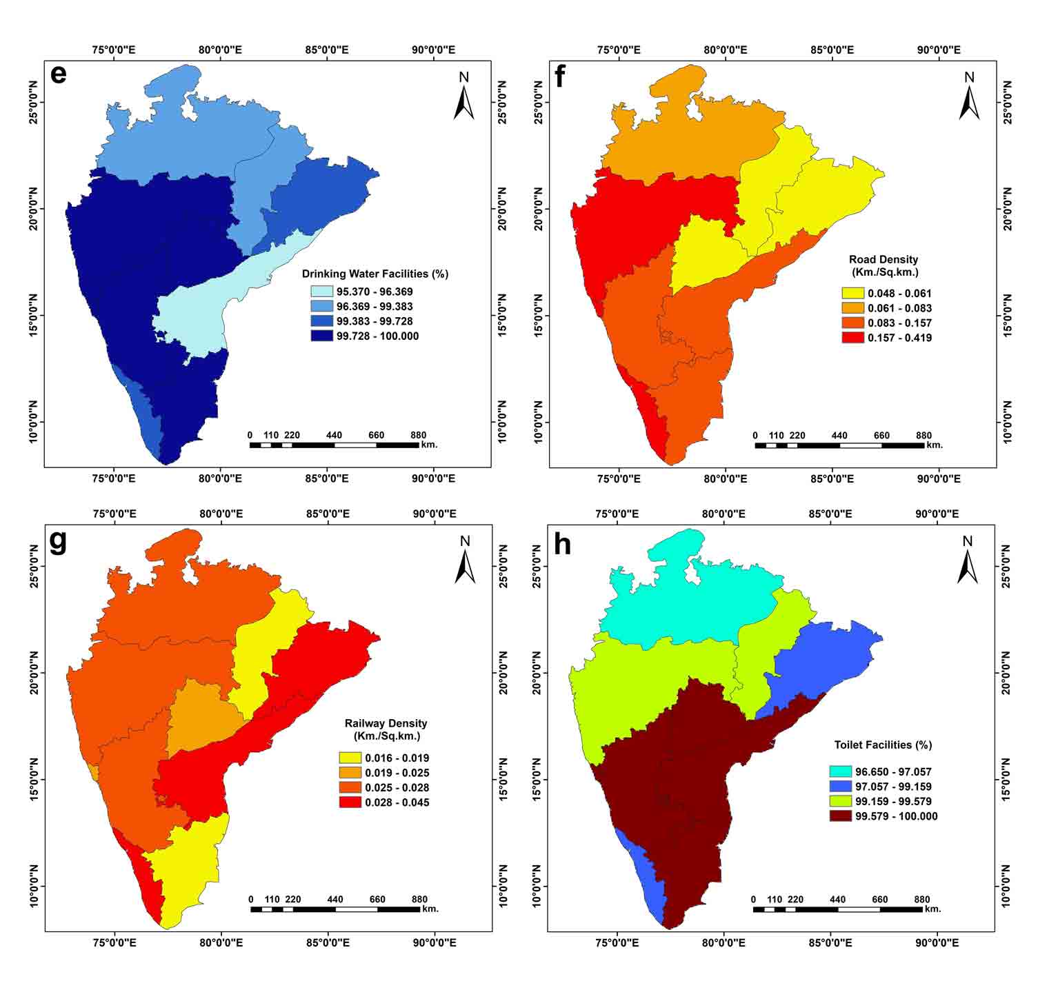
4.2.2 Drinking water facilities

Almost all educational institutions of Odisha, Maharashtra, Goa, Karnataka, Kerala, Tamil Nadu and Telangana states were found drinking water facilities (99.383% to 100%). On the other hand, drinking water facilities (%) were relatively low for Madhya Pradesh, Chhattisgarh and Andhra Pradesh states (95.370% to 99.728%). The potentiality of education was positively influenced by the drinking water facilities (%) (Figure 6e). Thereafter, drinking water facilities (%) were categorized here into four groups and as the class value increases, priority also increases (1-11.176% area,3-29.145% area, 5-12.566% area and 7-47.113% area) and vice-versa.

Figure 6. Other Social criteria: e) Drinking water facilities, f) Road density, g) Railway density and h) Toilet facilitie

4.2.3 Road densities

Maharashtra, Goa, Kerala, Karnataka, Tamil Nadu and Andhra Pradesh states were marked with 0.083 to 0.419 road densities. Relatively low road densities were found for the Madhya Pradesh, Telangana, Chhattisgarh and Odisha states. Here, the road density was classified into 4 groups i.e., 0.048 to 0.061, 0.061 to 0.083, 0.083 to 0.157 and 0.157 to 0.419 (Figure 6f). As the road density increases, the potentiality of education is also flourishing and vice-versa. Following this recommendation, 1 (25.102% area), 4 (20.716% area), 6 (31.730% area) and 8 (22.452% area) weightages were assigned to each class of road densities, respectively.

4.2.4  Railway densities

Within the study region, densities of railway varied from 0.016 to 0.045. Relatively low densities (0.016 to 0.025) were found for the Chhattisgarh, Telangana, Goa and Tamil Nadu states. High railway densities were found in the Madhya Pradesh, Maharashtra, Karnataka, Kerala, Andhra Pradesh and Odisha states. Railway densities positively influence the educational potentialities (Figure 6g). Here, densities of railway were grouped into 4 classes i.e., 0.016 to 0.019, 0.019 to 0.025, 0.025 to 0.028 and following the above recommendation, the above classes were recoded with 1 (19.290% area), 3 (6.789% area), 4 (52.638% area) and 5 (21.283% area) weightages, respectively (Table 11). Therefore, as the class value of railway densities increased, educational potentiality has also flourished and vice-versa.

4.2.5 Toilet facilities

Almost all educational institutions of Goa, Karnataka, Telangana, Andhra Pradesh and Tamil Nadu were marked with nearly 100% toilet facilities. On the contrary, 96.650% to 99.159% educational institutions in the states of Madhya Pradesh, Chhattisgarh, Maharashtra, Odisha and Kerala had toilet facilities. In an educational institution, the facilities of the toilet are essential (Figure 6h). So, it positively influences the potentiality of education. So, with increasing facilities of toilet, increasing weights were assigned, such as 1 (20.711% area), 4 (12.566% area), 6 (28.174% area) and 8 (38.548% area), respectively (Table 11).

4.3 Weighted Sum Models

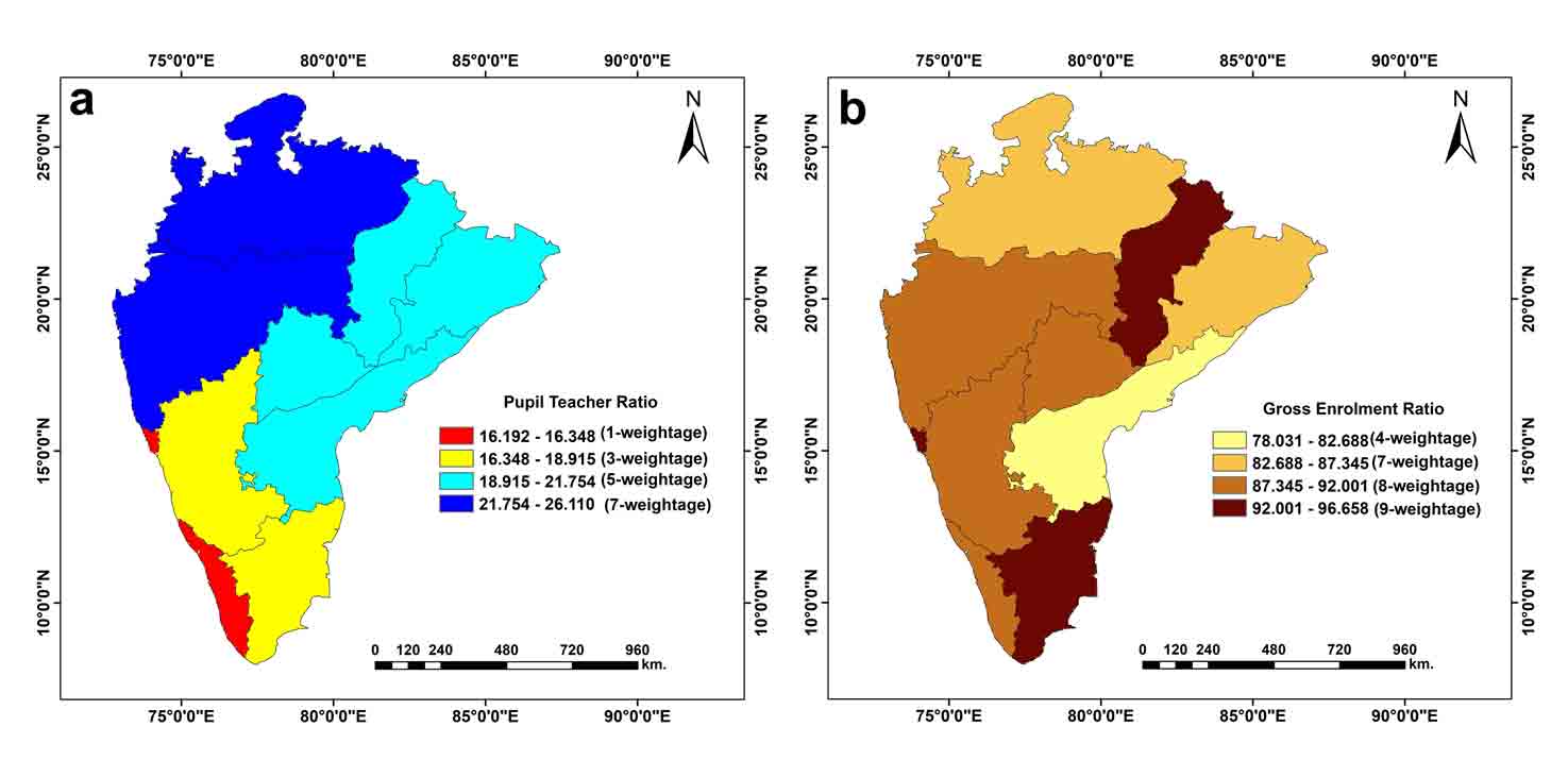
4.3.1Weighted sum model of PTR

PTR for the upper-primary level, primary level, secondary level, senior secondary level, university and colleges and university and constituent units were merged through different weights (Table 8). Here, the upper-primary level of education gained the highest priority (27.90% priority) followed by primary (27.30% priority), secondary (26.50% priority), university and colleges (6.30% priority), senior secondary (6.10% weightage) and university and constituent units (5.90% weightage). The potentiality of education was positively associated with PTR. Therefore, the weighted model of PTR was grouped into 4 classes and following the above recommendation, as the class values of PTR increase, the priorities also increase and vice-versa. Very strong importance (Code 7) was assigned for the Madhya Pradesh and Maharashtra states. Strong preference (Code 5) was marked for the Chhattisgarh, Odisha, Telangana and Andhra Pradesh states. The Maharashtra and Tamil Nadu states were marked with a moderate importance (Code 3). The Goa and Kerala states were noticed with an equal priority (Code 1) (Figure 7a).

Figure 7. Weighted sum model for a) Pupil-teacher ratio and b) Gross enrolment ratio

4.3.2 Weighted sum model of GER

GER for primary, upper-primary, elementary, secondary, senior-secondary, and higher education were integrated with different weights (Table 7). As a result, composite GER was formed. Here, the primary level of education was marked with the highest priority (42.50% weightage) followed by upper primary (24.10% weightage), secondary (17.81% weightage), senior secondary (6.00% weightage), higher education (4.80% weightage) and elementary (4.79% weightage). The GER positively influenced the potential of education. The weighted sum model for GER was classified into the 4 groups and as the class value increased, priority had also increased and vice-versa. For the composite GER, the extreme importance (Code 9) was assigned for the Chhattisgarh, Goa and Tamil Nadu states. Very strong to extreme importance was set for Maharashtra, Kerala, Karnataka and Telangana states (Code 8). Very strong significance (Code 7) was assigned for Madhya Pradesh and Odisha states and moderate to strong importance (Code 4) was marked for the Andhra Pradesh state (Figure 7b).

4.3.3 Weighted sum model of social

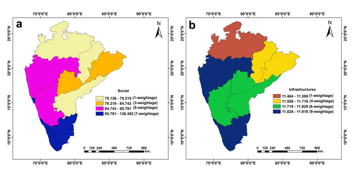
Gross Enrolment Ratio (GER), Pupil Teacher Ratio (PTR), literacy rate (%), population density and population growth rate were integrated to form the composite variable social (S). The variable social was in the positive association with the potentiality of education (Figure 8a). So, as the societal potential increased, priority has also increased (here 1, 3, 5 and 7, respectively) and vice-versa (Table 9). The weightage 1 was assigned for the Madhya Pradesh, Chhattisgarh and Andhra Pradesh states. Odisha and Telangana states were marked with the moderate importance (Code 3). Madhya Pradesh and Karnataka states were noticed with strong importance (Code 5). Goa, Kerala and Tamil Nadu states were marked with the very strong preference (Code 7).

Figure 8. Weighted sum model for a) Social category and b) Infrastructure category

4.3.4 Weighted sum model of infrastructural facilities

The weighted sum model for infrastructural facilities was prepared with the help of institution densities (51.20% weightage), road densities (26.50% weightage), railway densities (10.70% weightage), drinking water facilities (7.20% weightage) and toilet facilities (4.40% weightage) (Table 10).  Infrastructural facilities positively influence the potential of education (Figure 8b). Following this recommendation, the composite infrastructural facilities was grouped into 4 classes i.e., 11.464 to 11.558 (20.568% area), 11.558 to 11.719 (18.468% area), 11.719 to 11.828 (30.120% area) and 11.828 to 11.919 (30.844% area). With the increasing number of facilities, the priority increases (1, 4, 6 and 9, respectively) and vice-versa.

4.4 Composite Education Index

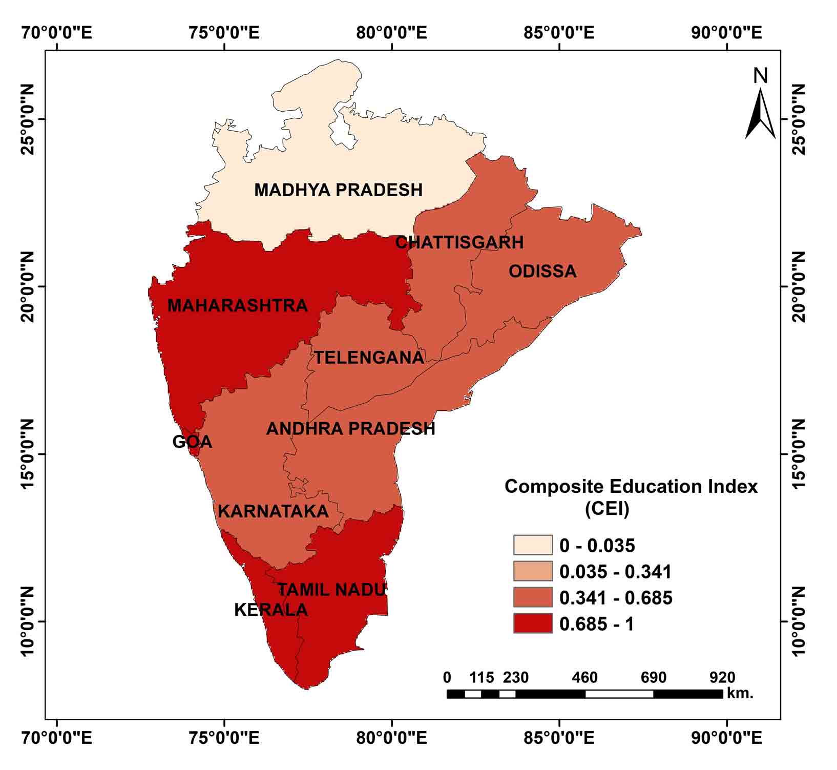
Overall, infrastructural facilities and social variables were merged to get the CEI. This CEI can be used to measure the educational potentialities. Here, the CEI was classified into 4 zones, i.e., zones with a very low score (VLS), zones with a low score (LS), zones with a moderate score (MS), and zones with a high score (HS). These zones were described as follows (Figure 9):

Figure 9. Composite Education Index

4.4.1 Zone with a very low index score

with very low index score implies the very low educational potentiality. The characteristics of this zone were discussed as follows:

• The entire area of Madhya Pradesh state was marked with very low CEI score (0 to 0.035) (Figure 9).
• Approximately, 29.03% area was marked under this zone.
• Pupil Teacher Ratio (Figure 4a to 4f) and Gross Enrolment Ratio (Figure 3a to 3f) were moderate in these portions.
• Literacy rate was relatively low in these portions of the study region (Figure 5a).
• Although population density (189 persons/km² to 236 persons/km²) was relatively low (Figure 5b) but the population growth rate (16.225 to 20.000) was high (Figure 5c) in these portions of the study region.
• The density of educational institution was relatively low (0.408 to 0.564, Figure 5d) in these sections of the study region.
• Drinking water facilities (Figure 5e), road densities (Figure 5f) and railway densities (Figure 5g) were also comparatively less in these sections of the study region,

As a result, the composite social and infrastructural facilities (Figure 8a and 8b) were also low in these portions of the study region.

4.4.2 Zone with a low index score

Zones with a low index score implies the low educational potentiality in any region. The characteristics of this zone were discussed as follows:

• The composite education score was comparatively low (0.035 to 0.341) for the entire sections of Odisha and Andhra Pradesh states (Figure 9).
• Although at primary level, Gross Enrolment Ratio (GER) was relatively high, but at the upper-primary, secondary, senior secondary and higher education enrolment of students was relatively low (Figure 4a to 4f) and as a result, in the composite GER, Odisha and Andhra Pradesh states were noticed with a comparatively less weights (Figure 3a to 3f).
• At all stages of education, PTR was comparatively low. As a result, the composite PTR was also noticed with the low weightages for the Odisha and Andhra Pradesh states (Figure 4a to 4f).
•  Relatively low literacy rates, high population densities and high population growth rates (Figure 5) were marked for the Andhra Pradesh and Odisha states.
• For the institution density (Figure 5d), performances of Odisha and Andhra Pradesh states were quite satisfactory.

4.4.3 Zone with a moderate and High score

Zones with high and very high index score implies the high educational potentiality. The characteristics of this zone were discussed as follows:

• The composite education score was comparatively high (0.341 to 0.685) for the entire sections of the Chattisgarh, Odisha, Andhra Pradesh, and Karnataka states (Figure 9).
• The composite education scores were the highest (0.685 to 1) for the Maharashtra, Kerala and Tamil Nadu states.
• Approximately, 38.647% area was included under the zone of the moderate score. Further, 11.074% area was included in the highest education score.
• Composite scores of Social (79.219 to 95.791) and infrastructural facilities (11.558 to 11.828) (Figure 8a and 8b) were moderate in these sections of the study area.
• The GERs were the comparatively high in these sections of the study area (Figure 3a to 3f).
• The PTRs were also comparatively high in these sections of the study area (Figure 4a to 4f).

5.5 Comparison of the Result with a Related Index

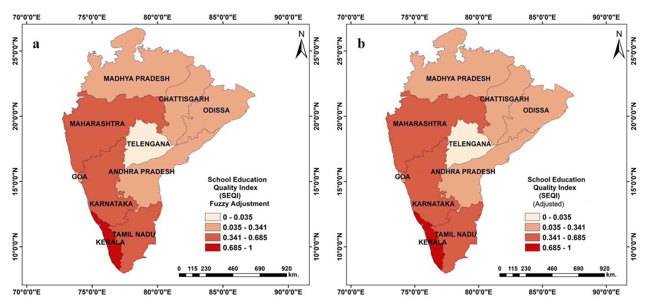
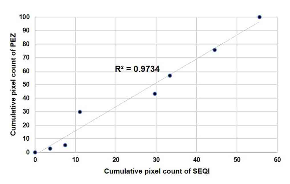
The composite education score was further validated with the School Education Quality Index (SEQI). Maharastra, Karnataka, Kerala, and Tamil-Nadu were noticed with comparatively high SEQI value (0.341 to 1), whereas the Madhya Pradesh, Chattisgarh, Odisha, Telangana and Andhra Pradesh were noticed with a comparatively low SEQI score (0 to 0.341) (Figure 10). The cumulative pixel count of SEQI and CEI were plotted in the X-axis and Y-axis respectively. The Correlation Coefficient value was obtained as 0.979 (Figure 10). Therefore, the composite education index can easily be utilized for the further analysis without any doubt.

Figure 10. School Education Quality Index (SEQI)

Figure 11. Validation of CEI with SEQI

5 . DISCUSSION

The remaining states were found with moderate educational performances. More importantly, this research has utilized an integrated multistep AHP procedure by linking two parameters, ten criteria, and twelve indicators to denote the educational potentialities of the South and Central Indian states. The composite structure of educational potentiality was completely neglected in previous research outputs done by other researchers. Therefore, the methodology adopted in this research has a wider applicability to measure the educational performances of an academic institution

The application of CEI in different sectors can vary across different educational sectors and contexts. When evaluating the quality of elementary and secondary education, CEI takes into account variables such pupil-teacher ratios, gross enrollment rates and infrastructural quality. The CEI is also effective in resource allocation and effective distribution. By identifying places or schools with lower CEI ratings, which may need more assistance and investment, governments and politicians may utilize CEI to distribute resources more effectively. The CEI can be used to assess the long-term effects of educational policies and changes. Changes in CEI scores can be used to evaluate the efficacy of certain arbitration. CEI can be utilized to evaluate the impact of education policies and reforms over time. Changes in CEI scores can help to gauge the effectiveness of specific interventions. The CEI can be asserted to assess the long-term effects of educational policies and changes. Changes in CEI scores may be useful to evaluate the efficacy of certain procedures. The CEI may be used to rate universities and institutions in higher education according to a variety of criteria, including infrastructure, faculty credentials with several social and infrastructural facilities. In order to assist students in making educated selections about where to attend school, CEI may be used to compare the standards of higher education institutions across various nations. By taking into account elements like job placement rates and industry relationships, CEI can evaluate how well vocational and technical education programs prepare students for the workforce. Institutions that provide vocational training can utilize CEI to pinpoint areas where their curricula and teaching strategies need to be improved. Taking into account elements like the accessibility of specialized resources and qualified staff, CEI may evaluate the inclusiveness of educational systems for students with disabilities. For kids with special needs, the CEI can be used to assess how well their Individualized Educational Plans (IEPs) are serving their educational requirements.

Although SEQI is already developed by NITI Ayog but this index is only capable to monitor the quality of primary and secondary educational levels. The CEI was developed by including diversified criteria and indicators in this research to monitor the educational potentiality at any regional level. Therefore, the CEI has more applicability and flexibility to assess the quality of the educational sector.

6 . CONCLUSION AND RECOMMENDATIONS

The research employed weighted sum and AHP approaches to build the CEI employing two parameters, ten criteria, and twelve indicators. Seven stages were necessary to complete the method, which also included creating a hierarchical structure, evaluating indicator independence, obtaining expert input for pairwise comparisons, estimating weight, and categorizing CEI into four groups using Jenk’s natural breaks. The CEI was subsequently changed to have a range of 0 to 1 and compared to SEQI, producing a high R-squared value of 97.3% that showed its efficacy in determining educational potential. A large number of criteria are merged in this index, and it is flexible and easy to implement in any region. However, future researchers and decision-makers should take the following factors into account while applying CEI:

• Education systems evolve with time, as do the results. The CEI must be updated often in order to correctly capture these changes. This might entail adding new indicators, changing weightings, or updating data sources.
• It should be clear to researchers how the index is put together, why certain indicators were chosen, and how weights are distributed.
• Be aware that different regions and environments might have quite different educational systems. Future studies should investigate the performance of the CEI at other levels of detail, such as the national, regional, or local level.
• Consult with educators, decision-makers, and other interested parties to get their opinions. Their suggestions can be used to improve the index and make sure that it reflects the difficulties and objectives of contemporary schooling.
• Utilize the CEI to analyze trends over time. For policymakers and scholars, tracking changes in educational access and quality can yield insightful information.
• Compare various areas, nations, or educational systems using the composite education index. Comparative analysis can point out areas for development and best practices.
• Make policy suggestions that are supported by evidence based on the findings of the composite education index. Determine the precise locations where actions are required to enhance educational results.
• Inform the public and decision-makers about the findings and consequences of the composite education index. Increased support for reform initiatives may result from improved understanding of the problems facing education.

Overall, the CEI is flexible and an integrated index to measure the educational potentiality across several higher education institutions as well as primary and secondary educational institutions.

Tables

Figures

Conflict of Interest

Acknowledgements

Abbreviations

References