Keywords

Watershed , Prioritization , Ranking , Multi-criteria analysis , Correlation matrix , Weights , Influence , AHP

1 . INTRODUCTION

Watershed is a hydrological unit (Swallow et al., 2001; Johnson et al., 2013). It is a unique bio-physical unit (Corn, 1993; Cannon, 2000) of Earth’s surface including morphology, soils, surface water, surface geology, near surface atmosphere, vegetation influencing potentials of land use and result of past and present human activity, etc. (Bhagat, 2012; Wani et al., 2008). Watershed contours the natural resources including soil, water, vegetation as well as socio-eco-cultural resources (Ghanbarpour and Hipel, 2011). In view of the depleting conditions of natural resources and increasing demands for meeting the requirements of the rapidly growing population, a holistic, well-planned long-term strategy is needed for sustainable watershed development and management (Perez and Tschinkel, 2003; Iqbal and Sajjad, 2014; Joshi et al., 2006; Wani et al., 2011; Gajbhiye et al., 2011). Therefore, many governments, non-governmental agencies and personalities have invested their energies for conservation of these resources. Some of them have used watershed management techniques to conserve soils, groundwater, vegetation, improve agricultural productivity (Shah and Gibson, 2013), increase soil moisture and protective irrigation (Bhagat, 2014; Joshi el al., 2004; Pokharkar, 2011), increase groundwater level (Evers and Lars, 2013; Ferrer et al., 2014), reduce soil (Bhattacharyya et al., 2015) and vegetation degradation (Perez and Tschinkel, 2003; Bishop et al., 2012; Kaur et al., 2014) with public participation (Perez and Tschinkel, 2003; Montz, 2008; Ghanbarpour and Hipel, 2011; Swami  et al., 2012; Shah and Gibson, 2013; Mitchella et al., 2014; Oel et al., 2014; Watson, 2014).

Watershed approach is the integration of protection and saving of resources (Rockstrom et. al., 2004). Many action projects have adopted this watershed approach (Ames et al., 2005; Tiwari et al., 2008) for conservation of natural resources including soil, water, vegetation, etc. as well as socio-cultural resources for enriching livelihood of rural peoples (Pangare, 1998; Willett and Porter, 2001; Ali et al., 2010; Mitchella et al., 2014).

Morphometric analysis of river basin provides useful information for monitoring the groundwater (Kaushal and Belt, 2012; Swami et al., 2012; Jankar and Kulkarni, 2013), surface water (Li, 2009), degradation of soil and vegetation. Morphometric analysis is measurements and analysis of linear, aerial and relief parameters in relation of land surface, shape and dimension (Singh and Singh, 2011; Iqbal and Sajjad, 2014; Raja and Karibasappa, 2016). Theses parameters have been widely used for prioritization analysis of watersheds at micro and regional scale.

Sridhar et al. (2012), Kothari and Garde (2016) and Mishra and Nagarajan (2010) have used morphometric parameters for prioritization of watershed. Further, scholars like Iqbal and Sajjad (2014) have added data of land use/land cover along with morphometric analysis for prioritization of watershed, while Gajbhiye et al. (2014) have used Sediment Yield Index estimated from RS and GIS approach for this purpose. Sepehr et al. (2017) have adopted morpho-hydrological approach with criteria like slope, flooding, climate, geomorphological phenomena and rainfall. However, Gumma et al. (2016) and Gashaw et al. (2017) have noted the limitations of watershed prioritization due to partial knowledge of hydrological classifications and invalid models for estimation of soil losses. Existing models of prioritization are based on morphometric analysis and ranking techniques. Therefore, present study focused on watershed prioritization using robust techniques like correlation analysis for selection of parameters, weighted index and influence analysis for prioritization of watersheds for planning, management and development. The methodology used in the study may be helpful in successful implementation of developmental projects as well as for monitoring the natural resources for sustainable development.

2 . STUDY AREA

The Kas basin (182.66 sq km) is the part of upper Mula Basin in hilly zone of Deccan plateau in Maharashtra (India) (Figure 1). The region enclosed Aa and pahoehoe basaltic lava flow. The height varies from 620 m to 1060 m. The average annual rainfall is 473 mm, varies from 777 mm at Bramhanwada to 358 mm at Bota. Kas (Figure 2) is tributary of river Mula and receives water from many minor streams. Shallow, very shallow, slightly deep well drained soils are observed with 68.03 % area under crop lands. About 93% basin area observed fine calcareous soil on gently sloping lands with severe and moderate erosion. Cereals like Bajra, Rice and different Pulses, Vegetables, Groundnuts are major crops in the kharip (rainy) season and Jawar, Wheat, Maize and Sunflower are major crops in rabbi (winter) season. Farmers use available surface water and groundwater for seasonal irrigation for vegetables and groundnuts. About 7.42% lands especially on hill slopes (Figure 5) are covered by sparse forests and 16.96% by shrubs and grasses. Majority of population in the region is living below poverty line and facing many problems for livelihood. The Kas basin has been divided into ten sub watershed namely SW1 to SW10 for analysis and prioritization (Zende et al., 2013).

Figure 1. Location map: Kas Basin

Figure 2. Drainage network

3 . METHODOLOGY

3.1  Database and Software

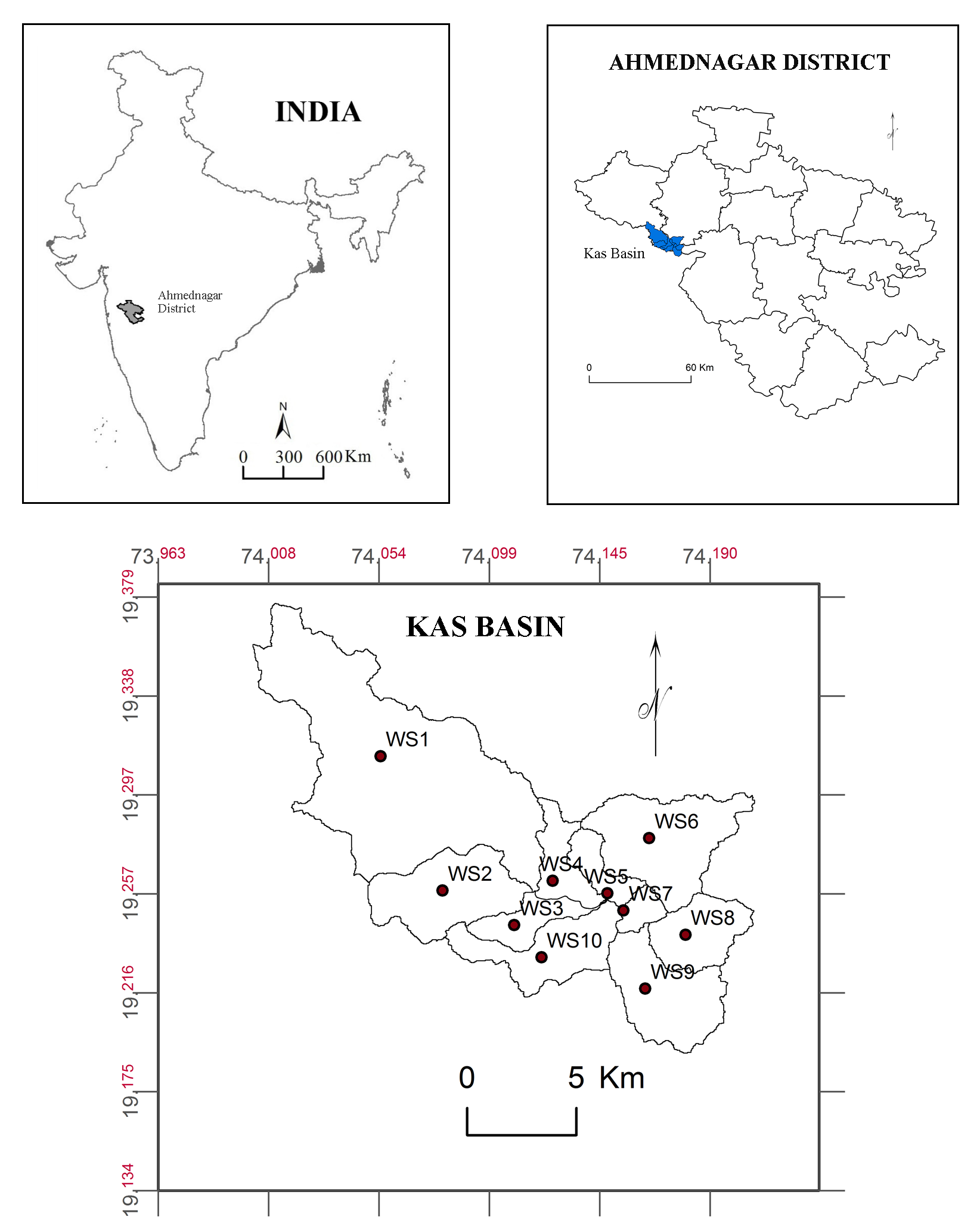
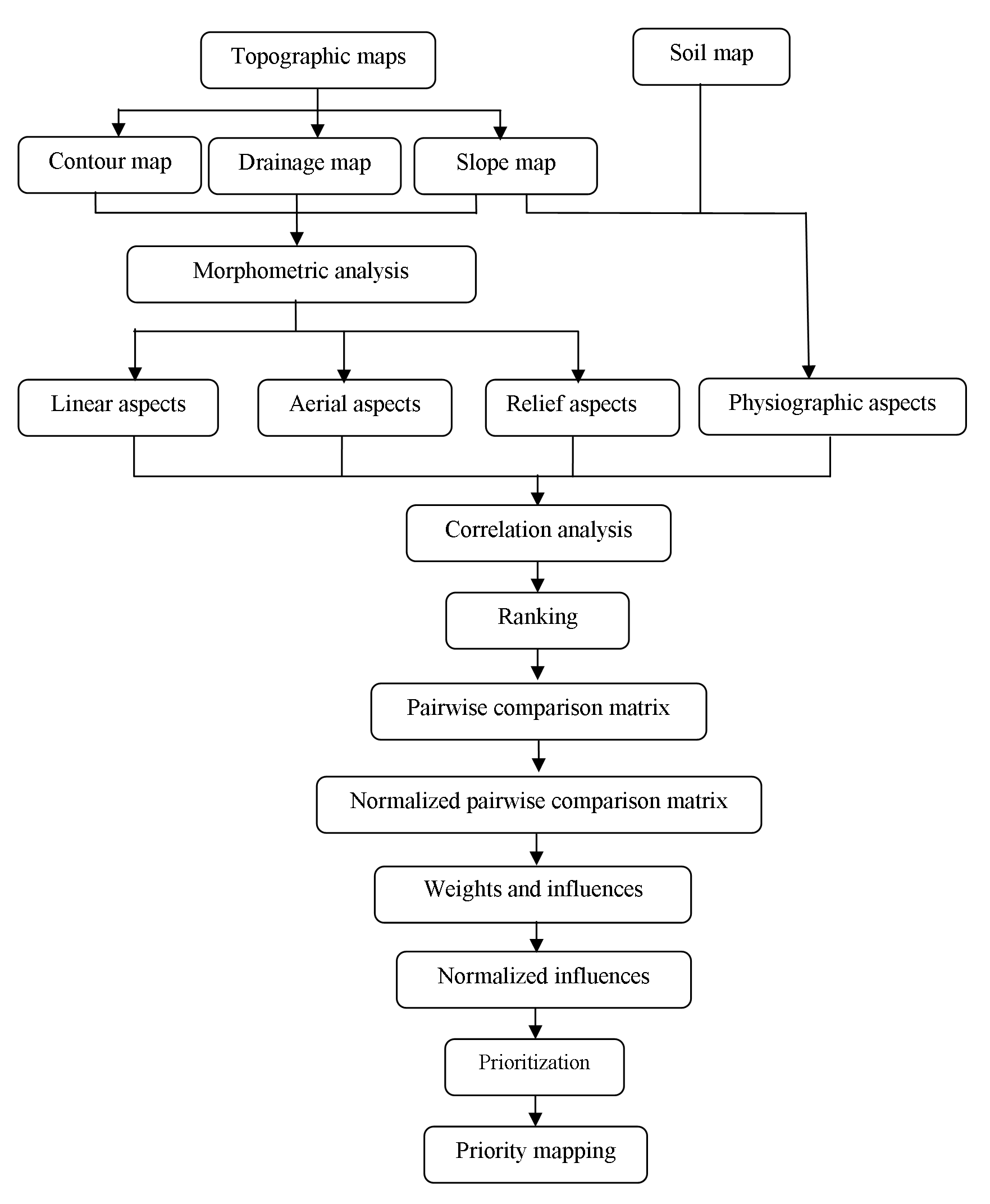
The present analysis (Figure 3) needs information of morphometric parameters, geological and soil characteristics of the region. Maps showing morphometric parameters (Table 1) including linear [Stream Order (\(U\)) , Bifurcation Ratio (\(R_b\)) , Stream Length (\(L_u\)) ], aerial [Basin Area (\(A\)) , Basin Length (\(L_b\)) , Basin Perimeter (\(P\)) , Drainage Density (\(D_d\)) , Stream Frequency (\(F_s\)) , Form Factor (\(R_f\)) , Circularity Ratio (\(R_c\)) , Elongation Ratio (\(R_e\)) , Compactness Coefficient (\(C_C\)) , Drainage Texture (\(D_t\))  ,Texture Ratio (\(T\)) , Drainage Intensity (\(D_i\)) ] and Relief [Relief Ratio (\(R_{h1}\)) , Ruggedness Number (\(R_n\)) ] were prepared from the topographic maps (47I/3 and 47I/4), SOI [survey of India]. ASTER DEM data was used for delineation of watershed boundaries. Geological map (Figure 4) was prepared using map procured from National Institute of Geological Survey, Nagpur (India). Soil map (Figure 6) procured from National Bureau of Soil Survey and Land Use Planning (NBSS and LUP), Government of India for preparation of soil map of Kas basin. Rainfall data was collected from Government of Maharashtra (India) for three rain gauge stations (1992-2013) located within the study area. Topographic, geological and soil map have been loaded and registered (Zeilhofer et al., 2008) in GIS software for preparation of maps.

Figure 3. Schematic preparation

3.2  Criterion

Morphometric properties (Zolekar and Bhagat, 2015) have close relationship with watershed planning, management and development. Gharde and Kothari (2016), Gabale and Pawar (2015), Ali and Ali (2014), Rao and Yusuf (2013), Rekha et al. (2011), Romshoo et al. (2012), Singh and Singh, (2011), Sharma et al. (2009), Vandana (2013), Zende et al. (2013), Aravinda and Balakrishna (2013) and Khare et al. (2014)  have used the linear, aerial and relief aspects of the prioritization of watershed. Rao et al. (2014), Aouragh and Essahlaoui, (2014), Raja and Karibasappa (2014) and Kiran and Srivastava (2014) have used linear and aerial aspects. Land use/land cover directly reflects the impact of geomorphology, slope, soil, land surface processes, climate, hydrology, etc. as well as human activities (Mishra and Nagarajan, 2010; Panhalkar, 2011; Romshoo et al., 2012; Gashaw et al., 2017). Therefore, Kaur et al. (2014) have used morphometric parameters in combination of land use analysis. Further, Gebre et al. (2015) have added information about changes in land cover and land use, soil type, soil texture with morphometric parameters. Gumma et al. (2014) have used the information of population, slope and rainfall with these parameters for prioritization of watersheds. Vulevic et al. (2015) have used all these parameters for prioritization of watershed using the multi-criteria decision analysis. Here, multi-criteria decision making based on analytical hierarchy process was performed using morphometric parameter and soils. Influences of criterion were calculated using estimated weights and these influence normalized using variations of criterion within selected watersheds. Rainfall is important parameter in prioritization analysis at regional level. However, selected sub-watersheds have no spatial variation in rainfall.

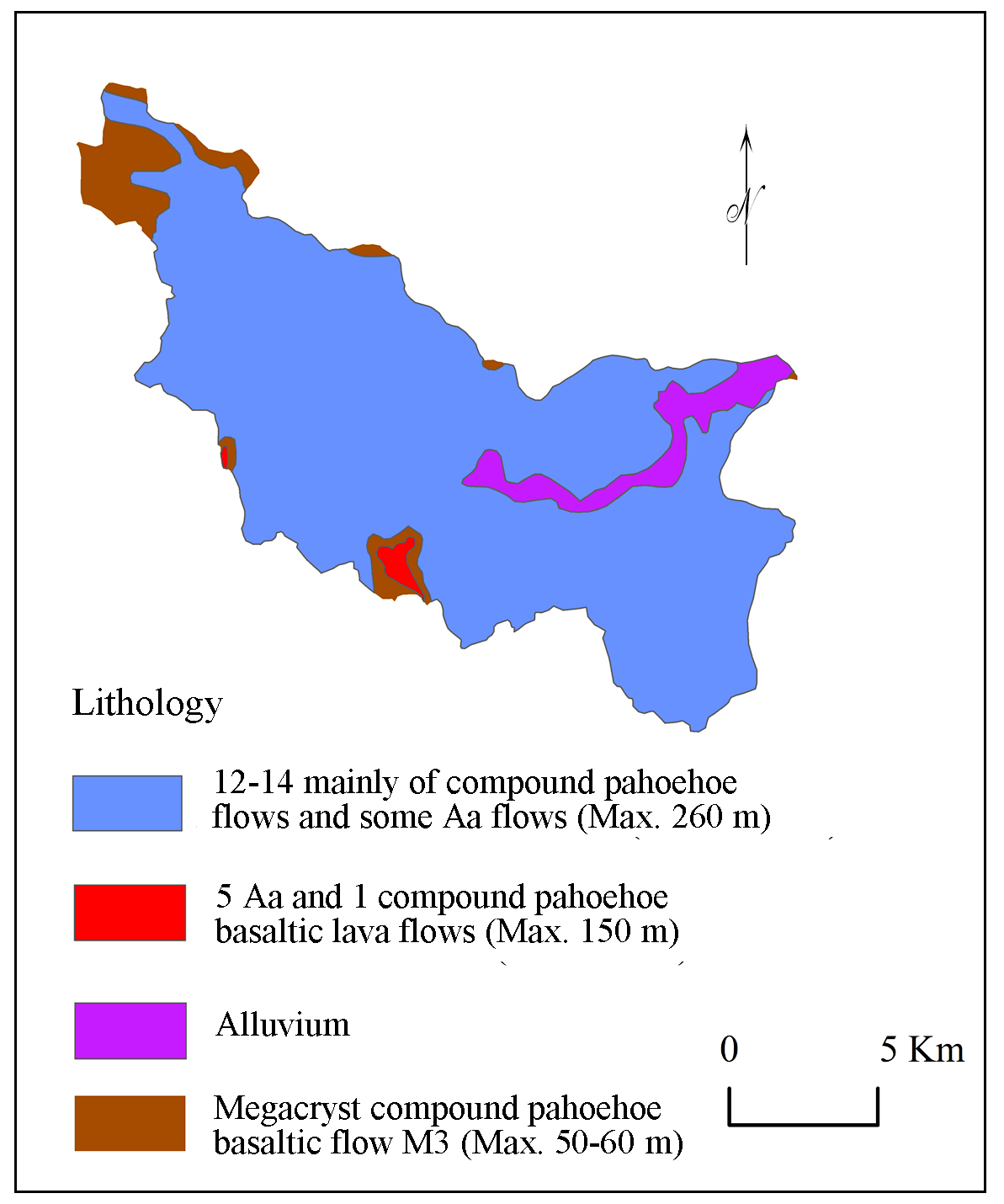
Geology of the region defines nature of subsurface materials, rate of infiltration, amount of runoff, level of ground water and hydraulic conductivity of the surface (Engelhardt et al., 2011; Olden et al., 2012; Dhanalakshmi and Shanmugapriyan, 2015). Bedrock permeability mainly depends on geology and water stability (Flint et al., 2013; Aouragh and Essahlaoui, 2014). Therefore, watershed characteristics are responsive to nature of geology of the region (Gharde and Kothari, 2016). The study area is the part of Deccan trap with 12 to 15 compound pahoehoe flows and some Aa flows (up to 260m), megacryast compound pahoehoe basaltic flows M3 (50 to 60m), 5 Aa and 1 compound pahoehoe basaltic flows M3 (up to 150m) and alluvium type geology (Figure 4). However, no significant spatial variation observed in the region.

Figure 4. Lithology

Figure 5. Slope

3.2.1  Linear Aspects

Khare et al. (2014), Rao et al. (2014), Aouragh and Essahlaoui (2014), Raja and Karibasappa (2014), Kiran and Srivastava (2014) and Farhan and Anaba (2016) have used linear parameters: stream order (\(U\)), stream length (\(L_u\)), mean stream length (\(L_{sm}\)) , (Wilson et al., 2012), stream length ratio, bifurcation ratio (\(R_b\)) . These parameters are related with land surface erodibility. Therefore, linear aspects of the study area: stream order (\(U\)) , stream number (\(N_u\)) , bifurcation ratio (\(R_b\)) , mean stream length (\(L_{sm}\))  and stream length (\(L_u\)) , are selected for analysis of selected watersheds for prioritization.

a. Stream Order (\(U\))

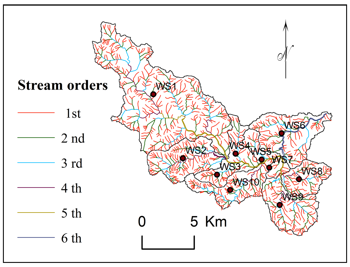
Stream orders indicate lithology, physiography, structure and uniformity of rocks in the watershed (Singh and Singh, 2011; Vandana, 2013; Chitra et al., 2011; Zende et al., 2013; Ali and Ali, 2014). Streams are appeared as the segments in GIS. The orders of these segments are calculated with the help of GIS software, Global Maper 11. About 79% streams (809) are recognized as first order  (Table 2), 16.11% (165) second order, 3.52% (36) third order, 0.78% (08), fourth order and 0.49 (05) fifth order. The sub-watersheds: WS1, WS2, WS3, WS4 and WS5 were delineated at fifth order of streams.

b. Bifurcation Ratio (\(R_b\))

Bifurcation ratio indicates the shape of basin, branching pattern, surface erodibility. Higher \(R_b\) values show an elongated basin whereas lesser represents circular basin (Chitra et al., 2011; Khare et al., 2014). It is the ratio between the total number of first order streams to that of the next higher order streams in the basin (Pareta and Pareta, 2011; Iqbal and Sajjad, 2014). The lesser values indicate less structural disturbances (Strahler, 1964) with stable drainage (Pareta and Pareta, 2011) (Table 2) whereas more values indicate a strong structural control over drainage system (Chitra et al., 2011). The bifurcation ratio varies from 2.97 to 6.74 and indicates higher erosion activity in the basin (Strahler, 1957; Rai at el., 2014) and need of soil conservation.

c. Stream Length (\(L_u\))

Stream length indicates surface run-off characteristics like slopes steepness, lithology and topography (Nongkynrih and Husain, 2011; Chitra et al., 2011; Iqbal and Sajjad, 2014). The stream length of each order of stream in Kas basin has been measured from topographic maps (Nagal, et al., 2014).  Longer streams have permeable bedrock and well-drained network (Kulkarni, 2015). Stream number and length are observed higher for first order and decreases according to increasing stream order. Total length of first order streams is estimated about 395.78 km (62.61%), second order streams 116.81 km (18.48%), third order streams 66.11 km (10.46%), fourth order streams 28.47 km (4.50%), fifth order streams 16.3 km. (2.58%) and sixth order streams 8.71 km (1.38%) (Table 3).

3.2.2  Aerial Aspects

Aerial aspects including basin area, basin length, basin perimeter, drainage density, stream frequency, form factor, circularity ratio, elongation ratio, compactness coefficient, drainage texture, texture ratio, drainage intensity and infiltration number are selected for the analysis.

a. Basin Area (\(A\))

Basin area is indicator of size (Strahler, 1957) and significant for calculating the drainage density (\(D_d\)) , stream frequency (\(F_s\)) , form factor (\(R_f\)) , circularity ratio (\(R_c\)) , elongation ratio (\(R_e\)) , compactness coefficient (\(C_C\)) and lemniscates (\(k\))  (Gabale and Pawar, 2015; Kothari and Garde, 2016). The Kas River drains over 181.65 km² (Figure 2) (Table 4).

b. Basin Length (\(L_b\))

Basin length indicates basin shape and hydrological characteristics (Chitra et al., 2011) including lemniscate’s value, form factor and elongation ratio (Pareta and Pareta, 2011; Nagal et al., 2014).  The basin length in the study area varies from 15 km (WS1) to 2.25 km (WS6) (Table 4). Maximum basin length indicates more texture, infiltration number and basin perimeter showing need of conservation.

c. Basin Perimeter (\(P\))

Basin perimeter is the length of outer boundary of the watershed forms the size, shape and drainage density (Strahler, 1957; Nagal et al., 2014). The perimeter of Kas basin is 85.19 km and varies for sub-watersheds from 69.82 km for WS1 to 9.95 km for WS4.

d. Drainage Density (\(D_d\))

Drainage density is useful for analysis of terrain, rocks, relief, soils, groundwater, erodibility and discharge of water and sediment (Pareta and Pareta, 2011; Engelhardt et al., 2011; Kaur et al., 2014; Gebre et al., 2015; Gabale and Pawar, 2015). Drainage densities in this watershed can be categorized (Gebre et al., 2015) as very coarse (2.17 to 3.92 km/km²) and moderate (3.29 to 4.18 km/km²) (Table 4). Higher values of \(D_d\)  indicates moderate slopes (Vandana, 2013; Argyriou et al., 2016) with semi-permeable hard rock, coarse textures, favorable conditions for groundwater conservation (Khare et al., 2014; Gebre et al., 2015; Gabale and Pawar, 2015). Drainage densities in Kas basin vary from 2.85 to 4.18 km/km² (Table 4).

e. Stream Frequency (\(F_s\))

Stream frequency indicates nature of subsurface materials, relief, infiltration rate, permeability, stream population, vegetative cover and have relationship with drainage density (Chatterjee and Tantubay, 2000; Pareta and Pareta, 2011; Singh and Singh, 2011; Chitra et al., 2011;  Romshoo et al., 2012; Vandana, 2013; Patel et al., 2013; Iqbal and Sajjad, 2014; Rai et al., 2014; Kaur et al., 2014; Gebre et al.,2015; Farhan and Al-Shaikh,  2017). Stream frequency depends on lithology, rock structure, subsurface permeability, infiltration capacity, relief, drainage network, rainfall, vegetation cover, etc. (Wilson et al., 2012; Aouragh and Essahlaoui, 2014; Gabale and Pawar, 2015; Kulkarni, 2015; Raja and Karibasappa, 2016; Argyriou et al., 2016). Sub-watersheds with dense forest show less frequency of streams in drainage network whereas agricultural lands show higher frequency (Zende et al., 2013). Stream frequency in the region varies from 2.31 to 6.47 km/km² (Table 4). Higher stream frequencies of WS2 (8.23), WS7 (6.47) and WS9 (6.93) indicate impermeability and less infiltration capacity of subsurface and higher relief with thin vegetation cover.

f. Form Factor (\(R_f\))

The form factor, \(R_f\)  indicates shape (Rai et al., 2014) and length of basin (Patel et al., 2013). The elongated watershed estimates less value and nearly circular watersheds show higher values (Gabale and Pawar, 2015). Perfectly circular watershed shows form factor about 0.75 (Pareta and Pareta, 2011). WS6 (0.56), WS7 (0.57) and WS8 (0.45) (Table 4) are nearly circular whereas WS1 (0.32), WS2 (0.38) and WS3 (0.35) are moderate elongated and WS4 (0.10) and WS9 (0.20) are more elongated. 

g. Circularity Ratio (\(R_c\))

Circularity ratio indicates flow of discharge, erosion, (Patel et al., 2013; Rao and Yusuf, 2013), stage of topography and shapes (Gray, 1961; Ali and Ali, 2014; Farhan and Anaba, 2016). Length and frequency of tributaries, geological structures, land use/land cover, climate, relief and slope of the basin affect the circularity ratio (Mishra and Nagarajan, 2010; Nongkynrih and Husain, 2011; Chitra et al., 2011; Iqbal et al., 2013; Kaur et al., 2014; Farhan and Anaba, 2016). Estimated circularity ratios (0.16 to 0.39) for watersheds in the region indicate high erosion with permeable homogeneous geology (Aravinda and Balakrishna, 2014; Wilson et al., 2012; Farhan and Anaba, 2016). Less circularity ratios for WS1 (0.20), WS3 (0.16), WS4 (0.19 and WS9 (0.20) indicate dendritic stage, whereas WS2 (0.31), WS5 (0.28), WS6 (0.36), WS7 (0.39) and WS8 (0.32) are comparatively mature dendritic streams (Table 4).

h. Elongation Ratio (\(R_e\))

Elongation ratio indicates shape, hydrology, slope, infiltration and runoff (Kaur et al., 2014; Iqbal and Sajjad, 2014; Zende et al., 2013; Wilson et al., 2012; Chitra et al., 2011; Mishra and Nagarajan, 2010). Elongation ratio is the ratio between the diameter and the maximum length of the basin (Nongkynrih and Husain, 2011; Strahler, 1964). Higher elongation ratios show more infiltration capacity of land surface and less runoff (Iqbal and Sajjad, 2014). WS6 (0.84) and WS7 (0.85) show oval shapes with more infiltration capacity of land surface; WS2 (0.70), WS5 (0.72) and WS8 (0.76) show less infiltration capacity and more runoff, whereas WS1 (0.64), WS3 (0.67), WS4 (0.36) and WS9 (0.51) show nearly elongated shape with less runoff and more infiltration. Therefore, watershed with higher relief and steep slopes should be selected for conservation purpose with high priority (Table 4).

i. Compactness Coefficient (\(C_C\))

Compactness coefficient indicates erosion risk and relationship of hydrology of the basin (Ali et al., 2014; Iqbal et al., 2013). Nagal et al. (2014) and Patel et al. (2013) have described the compactness coefficient dependent on size and slope in the watersheds. Estimated compactness coefficients in the study area vary from 1.60 to 2.48. WS1 (2.26), WS3 (2.48), WS4 (2.28) and WS9 (2.25) show high compactness coefficient which indicate less elongation and high erosion whereas WS2 (1.79), WS5 (1.90), WS6 (1.67), WS7 (1.60) and WS8 (1.76) show more elongation and less erosion (Table 4).

j. Drainage Texture (\(D_t\))

Drainage texture indicates lithology of the watershed (Rao and Yusuf, 2013). Drainage texture shows influence of climate, vegetation, rock, soil, infiltration capacity, relief, etc. (Kulkarni, 2015; Aouragh and Essahlaoui, 2014; Vandana, 2013; Iqbal et al., 2013; Chatterjee and Tantubay, 2000). Smith (1950) has been classified drainage density into five categories of drainage texture. The watersheds in the study area: WS3, WS4, WS5, WS6, WS7, WS8 and WS9 show coarse drainage texture (1.28 to 5.65). WS1 (5.49) and WS2 (5.65) indicate intermediate texture (Table 4) which are favorable for resource conservation.

k. Texture Ratio (\(T\))

Texture ratio indicates morphometric structure, runoff and drainage texture of the basin (Farhan and Anaba, 2016; Nagal et al., 2014). It depends on lithology, infiltration capacity and relief in the region (Farhan and Anaba, 2016, Khare et al., 2014; Rekha et al., 2011; Pareta and Pareta, 2011). WS1 (5.49) and WS2 (5.65) show higher texture ratio with high relief and intermediate topography; WS4 (1.28) and WS6 (1.31) show very coarse texture and WS3 (2.13), WS5 (3.54), WS7 (3.76), WS8 (3.69) and WS9 (3.30) show course topography and moderate runoff. Estimated ratio values are classified into four categories after Smith (1950).

l. Drainage Intensity (\(D_i\))

Drainage intensity indicates runoff, flooding, gully erosion, landslides and denudation of the basin (Gabale and Pawar, 2015; Pareta and Pareta, 2011). The drainage intensity is the ratio between stream frequency and drainage density (Nagal et al., 2014). Drainage intensity in the study area varies from 1.46 to 2.03 (Table 5). Watersheds in the region indicate small influence of drainage density and stream frequency.

m. Infiltration Number (\(I_f\))  

Infiltration number indicates infiltration characteristics, runoff, vegetation cover and permeability of soil cover (Nagal et al., 2014; Rao and Yusuf, 2013; Ranjan, 2013; Singh and Singh, 2011). Normally infiltration number of any watershed is defined as the product of drainage density and stream frequency (Nagal et al., 2014).  Infiltration numbers vary from 13.30 to 33.32. WS1 (15.41), WS3 (16.79), WS5 (16.46) and WS6 (14.52) show more runoff during rain spells.

3.2.3  Relief Aspects

a. Relief Ratio (\(R_{h1}\))

Relief ratio is important to understand overall slope, relief and erosion process in the watershed (Strahler, 1957; Chatterjee and Tantubay, 2000; Sharma et al., 2009; Engelhardt et al., 2011; Wilson et al., 2012; Vandana, 2013; Kaur et al., 2014; Yunus et al., 2014). The relief ratio is defined as the ratio between the total relief of a basin and the longest dimension of the basin similar to the main drainage line (Nagal et al., 2014). Relief ratios in the region vary from 0.07 to 0.34 (Table 4). The relief ratio normally increases with decreasing drainage area and size of the basin. Relief ratios for WS1, WS2, WS3, WS4, WS5, WS8 and WS9 indicate moderate slopes whereas WS6 (0.21) and WS7 (0.34) show high relief ratio.

b. Ruggedness Number (\(R_n\))

Ruggedness values indicate nature of relief, drainage density, slope, soil erosion, topography, lithology and discharge through the streams (Chitra et al., 2011; Pareta and Pareta, 2011; Rao et al., 2004; Nagal et al., 2014; Aouragh and Essahlaoui, 2014). The ruggedness number is the product of basin relief and drainage density. It is usefully relationship with steepness and length to understand the relief and drainage density   (Kaur et al., 2014; Nagal et al., 2014). Higher \(R_n\)  indicates irregular topography, lithological heterogeneity, high drainage density and high soil erosion. \(R_n\)  values for WS4, WS5 and WS6 are moderate indicating flat surface, moderate degree of dissection and soil erosion.

3.2.4  Physiographic Aspects

a. Slope

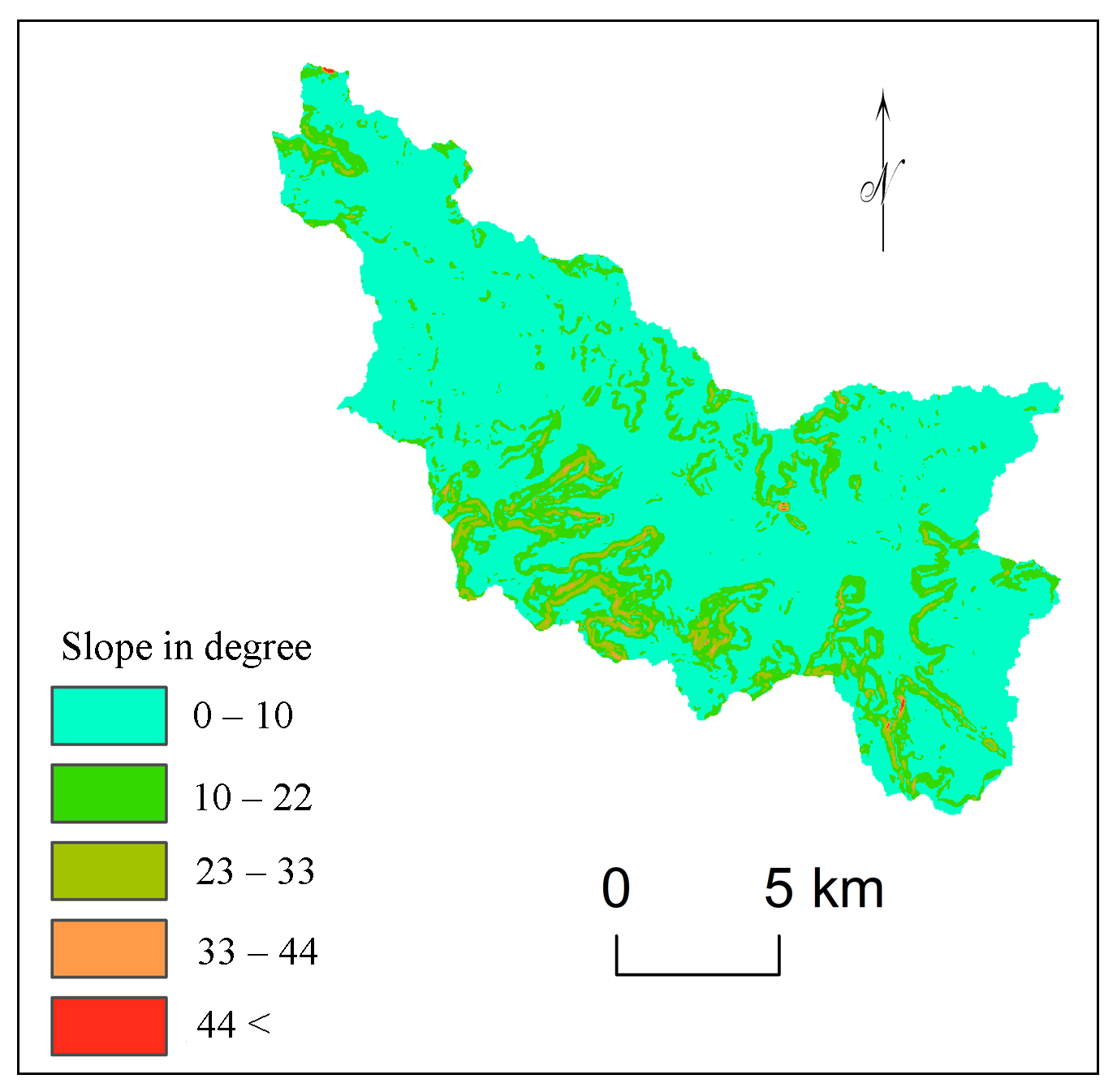
Slope analysis is helpful to identify the potential sites for watershed management (Zolekar and Bhagat, 2015; Argyriou et al., 2016). Slope is significantly affecting the morphometric aspects and drainage characteristics in the region (Kothari and Garde, 2016; Patel et al., 2013). Slope plays key role in formation of amount of runoff, rate of infiltration (Sepehr et al., 2017), drainage density (Nagal et al., 2014; Kaur et al., 2014; Argyriou et al., 2016; Rekha et al., 2011; Wilson et al., 2012), intensity of flood, quantity of erosion (Chang et al., 2013), soil depth, etc. The gentle slope shows less potentials of construction for water storages (Emamgholi et al., 2007). Land with moderate slope (10^º-22^º) is more suitable for conservation of resources and key criterion in watershed management. Therefore, area with moderate slopes was considered as the criterion for analysis of sub-watershed prioritization in the study area.

b. Soil

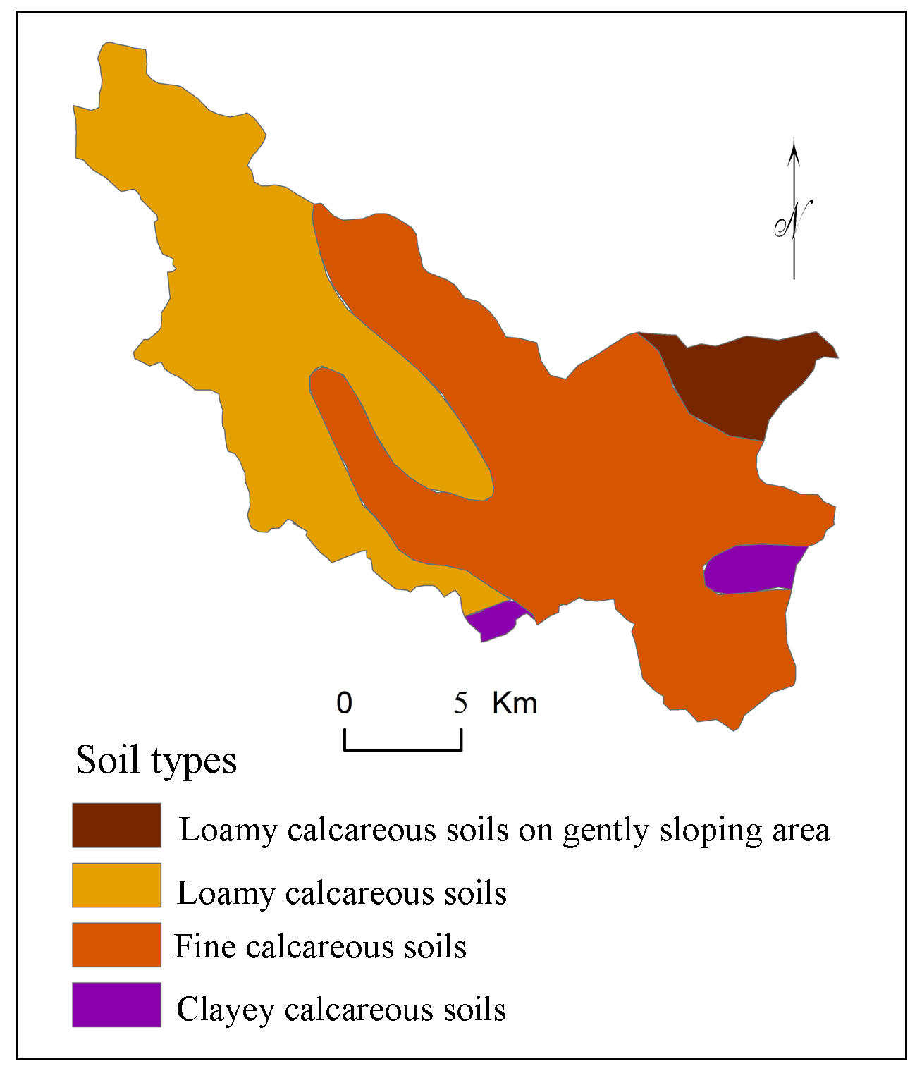
Soil is vital natural resources supporting life systems and socio-economic development (Ranjan, 2013). Soil erosion is a major problem in rain-fed area. Erosion of the top soil layer leads to constant land degradation and decline of soil quality and productivity (Farhan and Anaba, 2016; Yeole et al., 2012). Soil characteristics (Capodici et al., 2013) like texture, structure, organic matter content and permeability are useful to interpret the soil erodibility (Shinde et al., 2010). Soil map for Kas basin is prepared from map procured from National Bureau of Soil Survey and Land Use Planning (NBSS and LUP), Government of India. Clayey, loamy, calcareous, fine-loamy and fine calcareous soils are observed in the study area (Figure 6).

Figure 6. Soils

3.3  Analytical Hierarchy Process (AHP) for Watershed Prioritization

Prioritization of sub-watersheds was processed using AHP in six steps: (1) determination of rank, (2) pairwise comparison matrix, (3) preparation of normalized pairwise comparison matrix, (4) calculation of weights and influence, (5) normalization of influence and (6) prioritization of watersheds.

3.3.1  Determination Rank

Quantitative and qualitative methods have been widely used for determination of ranks to the parameters selected for weighted analyses. Scholars likes Sepehr et al., (2017), Ghanbarpour and Hipel, (2011), Rekha et al., (2011), Feizizadeh el al., (2014), etc. have used multi-criteria decision-making and pair wise comparison matrix. Zolekar and Bhagat (2015) have used expert opinions and correlation techniques for ranking the parameters in AHP based weighted overlay analysis for land suitability analyses. Bhagat (2012) has expressed that the correlation analysis is useful for better understanding of unstandardized parameters than the standardized parameters. Here, ranks of selected criterion have been determined based on sum of significant correlation coefficients estimated within the groups of criterions (Table 5).

Correlation between different 19 physiographic and morphometric parameters (Table 4) estimated using Pearson’s correlation technique (Yin et al., 2012) (Table 5). Yunus et al. (2014) and Farhan and Al-Shaikh (2017) have classified significant correlation values into three categories: strong correlation (0.8 to 0.9), good (0.7 to 0.8), moderate (0.5 to 0.7) and less than 0.5 insignificant (Table 5). Criterion selected for this study assigned ranks from 1 to 19 based on sum of the calculated significant positive correlations within the groups (Ranjan, 2013; Zolekar and Bhagat, 2015; Farhan and Anaba, 2016; Argyriou et al., 2016). Drainage Texture (\(D_t\)) , Texture Ratio (\(T\)), Bifurcation Ratio (\(R_b\)) , Geology and Stream Length (\(L_u\))  show more influence on erosion in hilly and foothill zones, therefore they are ranked 1 to 5, respectively. The criterion like Slope, Basin Area, Basin Perimeter, Ruggedness Number and Stream Frequency show moderate influence on surface erosion. They are ranked from 6 to 10 and further, Infiltration Number, Basin Length, Drainage Density, Drainage Intensity, Soil, Elongation Ratio, Form Factor, Compactness Coefficient and Relief Ratio were assigned ranks according to sum of significance values (Table 6).

3.3.2  Pairwise Comparison Matrix (PCM)

Pairwise comparison matrix has been performed (Table 7) to calculate the weights for calculation of influence of criterion (Zolekar and Bhagat, 2015) on the surface erosion (Elaalem, 2012). The PCM helps to understand the relationship between the criterion in relation to surface erosion and influence in assessment for applications of conservation techniques in the watershed (Emamgholi et al., 2007; Ranjan, 2013). The criterion values in PCM were divided by total of the column to find the cell values in normalized pairwise comparison matrix (Table 8).

3.4 Calculation of Weights and Influences

Average of values of criterions in row of normalized pairwise comparison matrix was calculated to get the weights of criterion (Zolekar and Bhagat, 2015; Maddahi et al., 2017) (Table 9). Further, influence of the criterion in formation watershed structure was estimated by calculating the cell values in percentage (equation 1) (Table 9).

\(C_i = \frac {W_c}{W_s} \times 100\)       (1)

\(C_i\)  = Normalized influence of criterion based on AHP.

\(W_c\)  = Estimated weights of criterion.

\(W_s\)  = Sum of estimated weights for all criterions.

\(C_i\)  indicates the share of criterion in total influence (100%) of criterion in formation watershed. This influence distributed within the criterion according to estimated weights in AHP analysis.  

3.4.1  Watershed Based Normalized Influence of Criterion 

The influence of criterion interprets the share of criterion in influence of criterion (100%) in formation of watershed. However, prioritization of watershed involves all parameters which may be uniformly distributed in selected sub-watersheds 

(Silva et al., 2007). Perez-Pena et al. (2009) and Argyriou et al. (2016) have proposed methodology to calculate the influence of morphometric and physiographic parameters for prioritization of the watersheds. Therefore, watershed wise influence of criterion was normalized according to spatial distribution of criterion in selected sub-watersheds (equation 2):

\(NI_w = \frac {C_w}{C_s} \times C_i\)        (2)

\(NI_w\)  = Watershed wise normalized influence.

\(C_w\)  = Cell value of criterion for the watershed.

\(C_s\)  = Sum of cell values of criterion.

\(C_i\)  = Estimated influence of criterion based on AHP.

3.4.2  Weighted prioritization

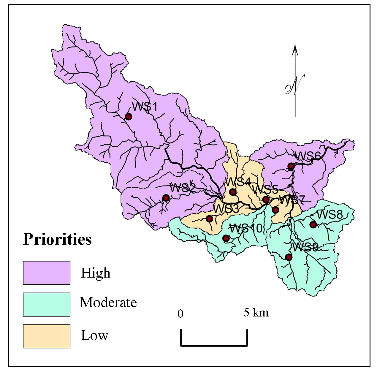
Several scholars have described the watershed prioritization by using morphological characteristics for management, planning and conservation of resources in the watershed. These parameters are linear, areal and shape based. These parameters decide the level of soil and water degradation therefore useful for assessment and prioritization of sub-watersheds (Aher et al., 2014). Prioritization of sub-watersheds in the study area was performed based on normalized pairwise comparison matrix (Table 10) (Ghanbarpour and Hipel, 2011), calculated influences for criterion and watershed wise normalized influence for criterion. Linear parameters are directly related to the erodibility factors and areal aspects represent inverse relationship (Aher et al., 2014).

\(P_w=\displaystyle\sum_{i=1}^{n} NI_w\)             (3)

\(P_w\)  = Periodization of watershed

\(NI_w\)  = Watershed wise normalized influence.

\(n\)  = Number of criterion

\(i\)  = Criterion

4 . RESULTS

Priorities of sub-watersheds for planning and development were calculated using multi-criteria based AHP method and calculated influences of criterions. Morphometric and physiographic criterions (19) were selected and ranked using correlation analysis for estimations of weights and influences. Estimated influences of criterions were normalized based on spatial distribution in selected sub-watersheds for prioritization. Estimated priorities were classified into three classes (Figure 7): high, moderate and low priorities.

4.1  Highly Priority

Sub-watersheds, WS1, WS2 and WS6 with first, second and third priorities are classified into the class, ‘Highly priority’ for planning and management of resources (Figure 7). These watersheds have gentle to moderate slopes with very shallow extremely drained loamy calcareous soils and severe erosion activities (Table 9). The productivity of these soils is very low and natural resources are exploited. 

Figure 7. Watershed priority classes

4.2  Moderate Priority

Watersheds: WS8, WS9 and WS10 were classified into the class, ‘Moderate priority’. Gentle slopes (27.80% area), calcareous soils with moderate erosion observed in these watersheds. Bifurcation Ratio and Texture Ratio indicate more surface erodibility and runoff from the basin which supports to more surface erosion. 

4.3  Low Priority

Watersheds: WS3, WS4, WS5 and WS7 show low drainage density, plain surface and low erosion activities with comparatively good agriculture. Well irrigation in rainy season is observed for commercial crops near to streams. Therefore, these watersheds are suggested with comparatively low priorities for planning and development.

5 . CONCLUSION

1. AHP based multi-criteria analysis is useful for prioritization of watersheds for planning, management and development.
2. Nineteen criterion i.e.\(R_b\), \(L_b \), \(A\), \(L_b\), \(P\), \(D_d\), \(P\), \(F_s\), \(R_f\), \(R_e\), \(C_C\), \(D_t\), \(T\), \(D_i\), \(I_f\), \(R_{h1}\), \(R_n\), slope and soil were selected for prioritization of sub-watersheds in the region.
3. Correlation analysis is useful for robust judgment for ranking the criterion for prioritization of selected watersheds.
4. Drainage intensity (27.80%), texture ratio (13.90%), bifurcation ratio (9.27%), geology (6.95%) and basin length (5.56%) show higher influence on nature of watersheds in the region.
5. Influences of criterion were estimated based on weights estimated using AHP methods. These values of influences are normalized using distribution of selected criterion within the sub-watersheds.
6. Watersheds were classified into three categories of priorities: high, moderate and low priorities.
7. The methodology formulated in this study can be efficient tool for rapid prioritization of watersheds for planning and management for development.

Tables

Figures

Conflict of Interest

Acknowledgements

Abbreviations

References