1 . INTRODUCTION
Groundwater plays an important role in water supply system for domestic, agricultural and industrial purposes in arid and semi-arid regions due to inadequate freshwater resources. It is estimated that approximately 65% groundwater used for drinking, 20% for irrigation and 15% for industrial uses in the world (Adimalla and Venkatyogi, 2018). According to United Nations Environment Programme (UNEP), one third of world population depends on groundwater for drinking particularly in India and China (UNEP, 1999). In India, groundwater is satisfying the basic needs of the society and recently overexploitation has considerable pressure on this finite natural resource due to increasing population, agricultural and industrial demands (Subramani et al., 2005). In general, the chemical composition of groundwater is influenced by natural and anthropogenic processes viz., amount of precipitation, evapotranspiration rate, soil inputs, rock-water interaction, residence time, agricultural runoff and discharges of domestic and industrial wastes, etc. (Todd, 1980; Pawar et al., 2008; Pawar et al., 2014; Mukate et al., 2017). The consumption of contaminated water has pose serious health risk due to water contaminants like fluoride, nitrate and arsenic toxicity to millions of people (Hossain et al., 2013; Pandith et al., 2017; Adimalla and Li, 2018). Therefore, evaluation and monitoring of groundwater resources is important to prevaricates any health risk and protection of groundwater quality in natural state because it vital for public health and socioeconomic growth of the region
(Naik et al., 2008). Several studies reported that hydrochemical behavior of water is an essential to ascertain the groundwater suitability for drinking and irrigation for better human health and agricultural productivity (Tóth, 1999; Panaskar et al., 2014; Mukate et al., 2015; Wagh et al., 2016a and b; Adimalla et al., 2018).
The complete consideration of groundwater suitability for irrigation is significantly based on total ionic content of the water such as Electrical Conductivity (EC), Sodium Adsorption Ratio (SAR), Percent Sodium (% Na), Sodium (Na), Calcium (Ca), Chloride (Cl), Residual Sodium Carbonate (RSC), Magnesium Adsorption Ratio (MAR), etc. (Yidana et al., 2010; Wagh et al., 2016a; Panaskar et al., 2016; Adimalla and Venkatayogi, 2018). In addition, it depends on salt concentration, sodium content, nutrients rate, alkalinity, acidity and hardness of water leads to loss of soil fertility and crop yield (Kirda, 1997). The poor water quality may influence the crop productivity physical condition of soil and high contents of dissolved ions in irrigation water will cause stunted plant growth and crop yield (Ayers and Westcot, 1994; Ramakrishnan, 1998). The Kadava river basin is prominent for production of cash crops like sugarcane, grapes, onion, pomegranates, vegetables, etc., due to sympathetic climate; thus, it becomes crucial to know irrigation suitability of groundwater. If groundwater quality is not protected well in time, the impact of using such contaminated water may result into the diminution of plant growth, agricultural yield and economical defeat (Ramesh and Elango, 2011). Therefore, identifying and addressing the irrigational water quality-related issues are essential to investigate at local to global scale. This study utilizes multivariate statistical techniques like Correlation Matrix (CM) and Principal Component Analysis (PCA) to identify influencing factors like geogenic and anthropogenic and there relative impacts on water quality variables. In recent times, GIS based interpolation techniques has been widely used to represent the spatiotemporal variation of ions, geomorphology, hydrogeology, land use pattern, etc., (Zolekar and Bhagat, 2015; Sahu et al., 2018). Also, hydrochemical characterization of groundwater has been evaluated through dominance of ion exchange, rock weathering, evaporation, etc., to distinguish the processes distressing the groundwater chemistry. moreover, these techniques widely applied by several researchers to know the chemical composition, source of ions and relation between different variables which persuade the water quality (Rao et al., 2014; Varade et al., 2018; Kant et al., 2018).
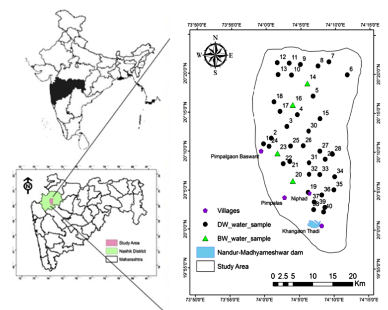
To ascertain the groundwater suitability for drinking and irrigation in the Kadava River Basin, also, it needs to understand the hydrochemical mechanisms which influencing the groundwater quality in basaltic terrain due to homogeneous lithological conditions and climatic deviation. In the study area, most of the inhabitants live in isolated villages and farm houses; where, dug and bore wells are regularly used for drinking and irrigation. The farmers use excessive fertilizers and agrochemicals to enhance crop productivity, which results downward leaching of contaminants along with recharge water, consequently, contaminated groundwater poses a serious health risk to human. Therefore, incessant monitoring and characterisation of groundwater quality is required to prevent further groundwater quality deterioration in the future. In the basin, very partial research has been embarked on groundwater quality and health related risk; however, studies by few federal government agencies and individuals addressed water quality issues (MPCB-NEERI, 2014; Wagh et al., 2017a and b; 2018a and b). Nonetheless, the connection between groundwater quality and its suitability coupled with hydrochemical mechanism was not investigated till recently. Therefore, the present study is initiated with main objectives of i) To ascertain the physicochemical characteristics of groundwater with a view to drinking and irrigation suitability; ii) To recognize the natural and anthropogenic factors which influencing on groundwater quality through multivariate statistical techniques. iii) To use of GIS based point interpolation technique to articulate the spatial extent of pollutants in the study area. Overall, integration of these techniques will help to find the source and influenced factors of water contaminants, as well, outcomes of the study may support to local water regulators to develop water suitability management plans in the Kadava river basin.
4 . RESULTS AND DISCUSSIONS
The summary of the groundwater parameters and comparison with the Bureau of Indian Standards (BIS) for drinking suitability is summarised in Tables 1 and 2.
Table 1. Physicochemical composition of groundwater samples (n=40)
|
Sample No.
|
Type
|
pH
|
EC
|
TDS
|
TH
|
Ca
|
Mg
|
Na
|
K
|
Cl
|
F
|
CO3
|
HCO3
|
SO4
|
NO3
|
IBE
|
|
G1
|
DW
|
7.8
|
1664
|
1081.6
|
590.41
|
48.1
|
114.72
|
60.4
|
1
|
68.46
|
0.5
|
300
|
60
|
37.87
|
50.14
|
-0.26
|
|
G2
|
DW
|
8
|
2336
|
1518.4
|
764.12
|
71.05
|
143.11
|
51.3
|
2.5
|
215.88
|
0.2
|
60
|
190
|
199.85
|
44.38
|
4.43
|
|
G3
|
DW
|
8.2
|
1414
|
919.1
|
354.85
|
50.1
|
56.02
|
63.8
|
1
|
110.76
|
0.1
|
40
|
120
|
87.82
|
50
|
4.4
|
|
G4
|
DW
|
8.4
|
816
|
530.4
|
302.68
|
51.3
|
42.56
|
26.5
|
4.6
|
108.28
|
0.3
|
20
|
140
|
22.61
|
19.38
|
3.62
|
|
G5
|
DW
|
8.3
|
1000
|
650
|
577.58
|
28.46
|
123.57
|
25.46
|
1.2
|
167.89
|
0.5
|
40
|
120
|
147.46
|
29.74
|
4.45
|
|
G6
|
DW
|
8.3
|
1426
|
926.9
|
454.28
|
50.5
|
80.04
|
42.1
|
1.5
|
119.36
|
0.4
|
20
|
120
|
145.14
|
61.7
|
4.38
|
|
G7
|
DW
|
8.2
|
1752
|
1138.8
|
473.89
|
53.73
|
82.85
|
42.7
|
1.5
|
126.88
|
1
|
20
|
110
|
166.28
|
51.81
|
4.48
|
|
G8
|
DW
|
8
|
4340
|
2821
|
1101.4
|
130.43
|
189.18
|
108.5
|
3
|
582.2
|
0.4
|
20
|
160
|
196.63
|
44.26
|
4.48
|
|
G9
|
DW
|
8.6
|
1024
|
665.6
|
367.98
|
30.46
|
71.21
|
15.6
|
3.5
|
42.6
|
0.5
|
100
|
90
|
39.51
|
40.54
|
3.93
|
|
G10
|
DW
|
8.2
|
2620
|
1703
|
671.26
|
71.36
|
120.26
|
53.4
|
1.5
|
223.06
|
0.2
|
40
|
120
|
197.8
|
51.91
|
4.06
|
|
G11
|
DW
|
8.4
|
1436
|
933.4
|
593.14
|
55.52
|
110.86
|
21.3
|
1
|
199.4
|
0.2
|
20
|
130
|
125.99
|
44.2
|
4.28
|
|
G12
|
DW
|
8.3
|
2620
|
1703
|
591.21
|
61.01
|
107.04
|
73
|
1
|
194.92
|
0.2
|
40
|
180
|
167.81
|
66.98
|
2.25
|
|
G13
|
DW
|
8.4
|
900
|
585
|
237.71
|
29.87
|
39.78
|
47.37
|
1.3
|
75.66
|
0.5
|
0
|
90
|
81.95
|
58.62
|
4.27
|
|
G14
|
BW
|
8.3
|
1664
|
1081.6
|
239.83
|
12.22
|
51.06
|
74.5
|
5.2
|
84.2
|
2
|
20
|
110
|
96.07
|
41.66
|
3.47
|
|
G15
|
DW
|
8.4
|
1083
|
703.95
|
389.44
|
33.63
|
74.51
|
31.36
|
7.5
|
145.6
|
0.6
|
0
|
160
|
58.65
|
57.63
|
2.39
|
|
G16
|
BW
|
8.5
|
992
|
644.8
|
237.65
|
32.06
|
38.43
|
52.4
|
1
|
61.12
|
0.1
|
40
|
140
|
52.69
|
59.94
|
-2.51
|
|
G17
|
DW
|
8.1
|
3770
|
2450.5
|
840.85
|
74.02
|
160.02
|
74.2
|
0.9
|
307.46
|
0.2
|
60
|
200
|
180
|
67.26
|
3.3
|
|
G18
|
DW
|
8.4
|
1844
|
1198.6
|
306.91
|
38.82
|
51.21
|
43.1
|
1.9
|
95.44
|
0.2
|
20
|
120
|
67.48
|
41.42
|
4.23
|
|
G19
|
DW
|
8.4
|
2198
|
1428.7
|
430.66
|
19.04
|
93.47
|
130.06
|
3.5
|
188.98
|
0.4
|
40
|
160
|
145.89
|
59.15
|
3.85
|
|
G20
|
BW
|
8.3
|
5680
|
3692
|
1281.79
|
44.89
|
285.37
|
299.8
|
1
|
627.64
|
0.5
|
300
|
200
|
172.91
|
53.49
|
4.38
|
|
G21
|
DW
|
8.2
|
2500
|
1625
|
497.5
|
33.05
|
101.23
|
65.02
|
1.1
|
159.82
|
0.4
|
40
|
140
|
155.95
|
59.65
|
1.76
|
|
G22
|
DW
|
8.1
|
1580
|
1027
|
189.73
|
29.47
|
28.32
|
150.33
|
1.3
|
239.67
|
0.4
|
0
|
120
|
69.51
|
42.35
|
-2.39
|
|
G23
|
BW
|
8.4
|
3414
|
2219.1
|
597.41
|
52.01
|
114.04
|
207.01
|
4.5
|
297.1
|
0.4
|
200
|
160
|
98.85
|
56.88
|
0.98
|
|
G24
|
DW
|
8
|
1368
|
889.2
|
572.18
|
68.15
|
98.04
|
52.3
|
1.5
|
197.78
|
0.3
|
40
|
180
|
158.89
|
58.99
|
-1.35
|
|
G25
|
DW
|
8.2
|
1774
|
1153.1
|
652.39
|
60.92
|
122.02
|
23.2
|
1.4
|
138.76
|
0.3
|
0
|
300
|
161.28
|
44.3
|
4.35
|
|
G26
|
DW
|
8.4
|
1689
|
1097.85
|
632.69
|
117.42
|
82.75
|
23.36
|
4.3
|
189.6
|
0.4
|
20
|
180
|
148.65
|
53.66
|
3.13
|
|
G27
|
DW
|
8
|
2400
|
1560
|
565.46
|
67.14
|
97.01
|
106.1
|
1.5
|
238.98
|
0.1
|
40
|
200
|
123.94
|
44.75
|
4.27
|
|
G28
|
DW
|
8.1
|
3244
|
2108.6
|
805.49
|
122.71
|
121.69
|
70.5
|
1
|
267.12
|
0.3
|
20
|
400
|
112.77
|
43.11
|
3.76
|
|
G29
|
DW
|
8.4
|
2314
|
1504.1
|
545.07
|
72.02
|
89.07
|
56.4
|
5.2
|
199.8
|
0.2
|
40
|
180
|
132.84
|
44.37
|
0.3
|
|
G30
|
DW
|
8.5
|
1638
|
1064.7
|
338.95
|
80.56
|
33.56
|
66.1
|
3
|
98.3
|
0.1
|
20
|
200
|
87.77
|
43.85
|
2.5
|
|
G31
|
DW
|
8.2
|
4060
|
2639
|
690.1
|
64.05
|
129.32
|
108.8
|
1.4
|
307.52
|
0.3
|
20
|
150
|
217.33
|
44.37
|
4.27
|
|
G32
|
DW
|
8.6
|
1640
|
1066
|
546.41
|
63.07
|
94.85
|
219.8
|
2.8
|
261.08
|
0.5
|
180
|
160
|
120.09
|
19.31
|
4.42
|
|
G33
|
DW
|
8.1
|
7080
|
4602
|
573.56
|
48.05
|
110.64
|
142.3
|
1.5
|
355.2
|
0.5
|
20
|
180
|
205.23
|
52.62
|
-2.95
|
|
G34
|
DW
|
8.8
|
1516
|
985.4
|
395.99
|
34.87
|
75.35
|
32.5
|
1.4
|
118.96
|
0.3
|
20
|
110
|
109.91
|
45.09
|
2.83
|
|
G35
|
DW
|
8.4
|
3410
|
2216.5
|
407.23
|
23.45
|
85.06
|
150.01
|
1
|
235.9
|
0.6
|
20
|
140
|
141.97
|
68.62
|
3.48
|
|
G36
|
DW
|
8.6
|
2014
|
1309.1
|
482.81
|
68.34
|
76.12
|
101.09
|
3
|
199.78
|
0.5
|
100
|
100
|
84.8
|
44
|
3.77
|
|
G37
|
DW
|
8.4
|
5100
|
3315
|
767.66
|
29.66
|
169.22
|
281.6
|
3.5
|
502.68
|
0.6
|
200
|
100
|
118.99
|
61.74
|
3.19
|
|
G38
|
DW
|
8.4
|
7760
|
5044
|
1033.99
|
38.08
|
229.07
|
583.4
|
4.5
|
1057.9
|
0.8
|
100
|
200
|
239.01
|
61.75
|
4.21
|
|
G39
|
DW
|
8.7
|
3240
|
2106
|
535.39
|
12.02
|
123.3
|
219.2
|
2.3
|
352.16
|
0.6
|
100
|
100
|
159.24
|
41.17
|
3.55
|
|
G40
|
DW
|
8.9
|
2020
|
1313
|
501.8
|
44.09
|
95.54
|
102.3
|
1
|
192.2
|
0.5
|
20
|
210
|
166.9
|
20.58
|
4.13
|
|
Minimum
|
7.8
|
816
|
530.4
|
189.73
|
12.02
|
28.32
|
15.6
|
0.9
|
42.6
|
0.1
|
0
|
60
|
22.61
|
19.31
|
-2.95
|
|
Maximum
|
8.9
|
7760
|
5044.0
|
1281.79
|
130.43
|
285.37
|
583.4
|
7.5
|
1057.9
|
2
|
300
|
400
|
239.01
|
68.62
|
4.48
|
|
Mean
|
8.3
|
2508.50
|
1630.53
|
553.49
|
52.89
|
102.79
|
102.45
|
2.32
|
233.90
|
0.43
|
60.00
|
155.75
|
130.11
|
48.63
|
2.90
|
G: Groundwater; DW: Dug Well; All the values are expressed in mg/l except pH on scale and EC in µS/cm.
Table 2. Groundwater suitability for drinking based on BIS drinking standards
|
Parameters
|
DL-PL
|
Samples above DL (%)
|
Sample numbers
|
Samples above PL (%)
|
Sample numbers
|
|
pH
|
6.5-8.5
|
100
|
1-40
|
15
|
9, 32, 34, 36, 39, 40
|
|
EC
|
-
|
-
|
-
|
-
|
|
|
TDS
|
500-2000
|
100
|
1-40
|
27.5
|
8, 17, 20, 23, 28, 31, 33, 35, 37, 38, 39
|
|
TH
|
300-600
|
90
|
1-12, 15, 17-21, 23-40
|
27.5
|
2, 8, 10, 17, 19, 25, 26, 28, 31, 37, 38
|
|
Ca
|
75-200
|
10
|
8, 26, 28, 30
|
0
|
|
|
Mg
|
30-100
|
97.5
|
1-20, 22-40
|
45
|
1, 2, 5, 8, 10, 11, 12, 17, 20, 21, 23, 25, 28, 31, 33, 37-39
|
|
Na
|
200
|
-
|
-
|
15
|
20, 23, 32, 37, 38, 39
|
|
K
|
12
|
0
|
-
|
0
|
|
|
Cl
|
250-1000
|
27.5
|
8, 17, 20, 23, 28, 31, 32, 33, 37, 38, 39
|
2.5
|
38
|
|
SO4
|
200-400
|
7.5
|
31, 33, 38
|
0
|
|
|
NO3
|
45
|
-
|
-
|
52.5
|
1, 3, 6, 7, 10, 12, 13, 15-17, 19-21, 23-24, 26, 34-36, 37, 38
|
|
F
|
1-1.5
|
2.5
|
14
|
2.5
|
|
DL: Desirable Limit; PL: Permissible Limit.
4.1 Groundwater Suitability for Drinking
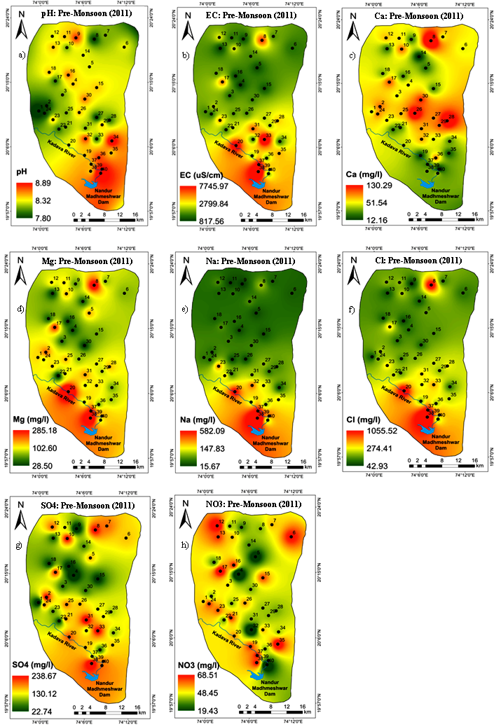
In the study area, pH values ranged from 7.8 to 8.9 with mean concentration of 8.3 which indicate groundwater is fairly alkaline. This nature is attributed to the loss of CO2, and the precipitation and dissolution of minerals from within the basalt (Kale and Pawar, 2012). Generally, elevated pH (alkaline waters) does not impact human health; but, it can alter the taste of the water and it shows a close association with ionic constituents of the water (Wagh et al., 2016a). As per the BIS Standards (2012), 15% (sample numbers 9, 32, 34, 36, 39 and 40) samples exceeded the permissible limit of pH (Table 2). In the study area, the spatial irregularity is observed in the Southern and Northern parts due to the influenced of saturation and dilution phenomenon (Figure 4a). The EC values varies from 816-7760µS/cm with mean concentration of 2508.5; however, it is related to the amount of total dissolved salts in water, which suggest an elevated inorganic pollution load in the water (Morrison et al., 2001). The value of EC increases with temperature and varies with the amount of soluble salts. The BIS has not prescribed any safe limit for EC; yet, the World Health Organization (WHO, 2011) designated 1500µS/cm EC as the permissible limit. The samples compared with WHO standards confirm that, 30 (75%) groundwater samples exceed the PL (Table 2). In view of spatial coverage, EC values are increased in the downstream portion of the Kadava River along the groundwater flow path, where alluvium deposits encountered with intense agriculture (Figure 4b). Total Dissolved Solids (TDS) is an important parameter for drinking and irrigation water suitability due to the contained ionic constituents (Davies and DeWiest, 1966). The TDS has a wide range of 530.4 to 5044.0 mg/L with mean concentration of (1630.53 mg/L) due to the semi-arid environment, lithology, agricultural and anthropogenic inputs. As per the BIS standards, all the groundwater samples exceed the desirable limit and 27.5% samples surpass the PL. High TDS is attributed from percolation of salts, dissolution of minerals from aquifer system and agricultural inputs and consumption such an elevated TDS content water may lead to gastrointestinal irritation (Panaskar et al., 2016).
The calcium content varies from 12.02 to 130.40mg/L (mean 52.89mg/L) (Table 1). According to BIS standards, all the groundwater samples are within permissible limit; hence, beneficial use for drinking. Conversely, 4 samples (numbers 8, 26, 28 and 30) are beyond the BIS desirable limit (75mg/L) (Table 2). Spatial distribution map demonstrated that high value of calcium occurred in patches of central and Southern parts due to local geological influences (Figure 4c). The magnesium content varies widely from 28.32mg/L to 285.37mg/L with mean value of 102.79mg/L. In the study area, 45% groundwater samples exceeded the PL (100mg/L) of the BIS. The high content of magnesium is encountered in patches of downstream of the Kadava River Basin catchment area (Figure 4d) owing to geological control and the presence of the Thakurwadi Formation containing picritic horizons (MgO of 3.5% to 11.86 %) (Beane et al., 1986). Average Ca+Mg value (meq/l) contributes 73.53% of total cations and signifies the major supply of mafic minerals such as olivine and pyroxene from weathering of basalt (Pawar et al., 2008; Rabemanana et al., 2005). TH content is ranges from 189.73-1281.79mg/L with mean value of 553.49mg/L (Table 1). As per the BIS standards, prescribed permissible limit of TH for drinking is 600mg/L. TH content of 27.5% (sample numbers 2, 8, 10, 17, 19 and 25, 26, 28, 31, 37 and 38) groundwater samples exceed the PL of drinking (Table 2). The sodium content of groundwater samples are ranges between 15.6mg/L to 583.4mg/L with mean 102.45mg/L. As per BIS standards, 15% samples (number 20, 23, 32, 37, 38 and 39) beyond the PL; hence, unfit for drinking (Table 2). The drinking of high content sodium water may cause human health effects like high blood pressure, arteriosclerosis, edema, hyperosmolarity, vomiting, etc (Prasanth et al., 2012). The high content of sodium is due to basalt weathering and dissolution of soil salts are redeposit by evaporation and sodium exhibits high solubility behavior (Stallard and Edmond, 1983). The high sodium content is likely derived from the Salher Formation which contains plagioclase feldspar and forms the solution between anorthite (CaAl2Si3O8) and albite (NaAlSi3O8) having a mole ratio of different cations and anions (Garrels and Christ, 1967). The South part has more accumulation of sodium due to the hydro-geomorphologic features such as slope and groundwater flow path (Figure 4e). The K content is varies from 0.9-7.5mg/L with mean value of 2.32mg/L, As per BIS standards, all the samples are within allowable range. However, high content in groundwater is mainly influenced by agricultural activities, which relies on K-rich fertilizers; however, its diminutive content is due to a lack of naturally-occurring K bearing minerals within the study area. The cation abundance in the study are descending order of Mg >Ca> Na>K.
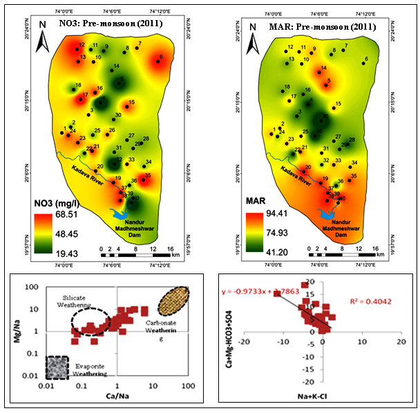
The chloride value ranges from 42.6-1057.9mg/L with mean value of 233.90mg/L (Table 1). As per BIS standards, 39 groundwater samples are within the PL, except sample number 38. Nonetheless, only 11 (27.5%) groundwater samples (numbers 20, 33, 37 to 39) exceed the DL for chloride (250mg/L) (Table 2). The high content of Cl in groundwater is contributed from natural and anthropogenic processes such as weathering of chloride minerals such as halite, domestic waste, fertilizers, etc. (Loizdou and Kapetnois, 1993). The spatial distribution map of Cl depicts that South part is mostly influenced by leaching of fertilizers and animal waste and agricultural runoff (Figure 4f). The sulphate content is varies from 22.61 to 239.01mg/L with mean value of 130.11mg/L (Table 1). It is observed that all of the groundwater samples are within the PL of sulphate; conversely, only 7.5% samples (numbers 31, 33, 38) exceed the DL (200mg/L) of drinking (Table 2). The source of sulphate content in groundwater is contributed from gypsum-containing fertilizers (Todd, 1980). The spatial variation map of sulphate demonstrated that the lower reaches of catchment area has been mostly affected; while, the northern region is influenced in few places, this area also has a prolonged agriculture and excessive use of fertilizers to increase crop yield (Figure 4g). The nitrate content varies from 19.31mg/L to 68.62mg/L with mean concentration of 48.63mg/L (Table 1). The analytical results compared with BIS standards confirm that 52.5% samples exceed the permissible limit (45mg/L) of the BIS (Table 2). The elevated nitrate concentration corresponds to nitrogen-phosphorus-potassium (NPK) complex fertilizers; Urea, animal excreta, domestic waste and organic compost (Wagh et al., 2017a; 2018a and b). The spatiotemporal map of nitrate illustrates the uneven distribution at South, Central and North region based on changing cropping pattern (Figure 4h). The fluoride content ranges from 0.1 to 2mg/L with mean concentration of 0.4 mg/L. The analytical results illustrated that only one sample (number 14) which contained 2mg/L fluoride; so, all the groundwater samples have allowable levels of fluoride for drinking as they show a fluoride content below the PL (Table 2). The fluoride content source is anthropogenic like phosphate fertilizer use in agricultural field. In general, anions in the groundwater are reflecting the influence of geochemical and anthropogenic inputs. It is illustrated that chloride is the primary anion followed by bicarbonate, sulphate and nitrate. The mean concentrations of all the anions are within permissible limits set by the BIS, except nitrate.
4.2 Irrigation Suitability of Groundwater
The absolute consideration of groundwater suitability for irrigation is significantly based on total ionic content of the water such as EC, SAR, % Na, Na, Ca, Cl, RSC, MAR, etc. In addition, it depends on salt concentration, sodium content, nutrients rate, alkalinity, acidity and hardness of water leads to loss of soil fertility and crop yield (Kirda, 1997). The area under investigation is renowned for agriculture due to sympathetic climate; thus, it is important to know water quality of irrigation. If groundwater quality is not protected properly then the impact of using such polluted water may leads to diminution of plant growth, crop productivity (Ramesh and Elango, 2011). As a result, the suitability of groundwater for irrigation has been attempted on the basis of various irrigation indices and their classification is represented (Tables 3 and 4).
Table 3. Irrigation suitability indices for groundwater
|
Sample No.
|
SAR
|
RSC
|
MAR
|
KR
|
Na(%)
|
SSP
|
|
G1
|
1.07
|
-0.98
|
79.90
|
0.22
|
18.14
|
18.00
|
|
G2
|
0.80
|
-10.36
|
77.05
|
0.14
|
12.91
|
12.60
|
|
G3
|
1.46
|
-3.87
|
65.08
|
0.39
|
28.07
|
27.89
|
|
G4
|
0.66
|
-3.15
|
58.03
|
0.19
|
17.21
|
15.86
|
|
G5
|
0.46
|
-8.42
|
87.86
|
0.09
|
8.85
|
8.63
|
|
G6
|
0.85
|
-6.56
|
72.54
|
0.20
|
16.89
|
16.60
|
|
G7
|
0.85
|
-7.12
|
71.99
|
0.19
|
16.50
|
16.22
|
|
G8
|
1.41
|
-19.00
|
70.74
|
0.21
|
17.70
|
17.47
|
|
G9
|
0.35
|
-2.65
|
79.58
|
0.09
|
9.34
|
8.34
|
|
G10
|
0.89
|
-10.29
|
73.74
|
0.17
|
14.80
|
14.59
|
|
G11
|
0.38
|
-9.22
|
76.89
|
0.08
|
7.34
|
7.16
|
|
G12
|
1.30
|
-7.69
|
74.52
|
0.27
|
21.09
|
20.96
|
|
G13
|
1.33
|
-3.33
|
68.94
|
0.43
|
30.33
|
29.99
|
|
G14
|
2.08
|
-2.40
|
87.44
|
0.67
|
40.94
|
39.96
|
|
G15
|
0.69
|
-5.27
|
78.69
|
0.17
|
16.47
|
14.73
|
|
G16
|
1.47
|
-1.18
|
66.64
|
0.47
|
32.41
|
32.16
|
|
G17
|
1.11
|
-11.76
|
78.28
|
0.19
|
16.02
|
15.92
|
|
G18
|
1.06
|
-3.57
|
68.74
|
0.30
|
23.65
|
23.19
|
|
G19
|
2.70
|
-4.78
|
89.11
|
0.65
|
39.66
|
39.28
|
|
G20
|
3.61
|
-12.75
|
91.38
|
0.50
|
33.41
|
33.37
|
|
G21
|
1.26
|
-6.46
|
83.62
|
0.28
|
22.06
|
21.89
|
|
G22
|
4.72
|
-1.87
|
61.56
|
1.70
|
63.15
|
63.03
|
|
G23
|
3.66
|
-2.81
|
78.52
|
0.74
|
42.96
|
42.65
|
|
G24
|
0.95
|
-7.29
|
70.57
|
0.20
|
16.65
|
16.42
|
|
G25
|
0.39
|
-8.30
|
76.95
|
0.08
|
7.33
|
7.09
|
|
G26
|
0.40
|
-9.15
|
54.01
|
0.08
|
8.10
|
7.37
|
|
G27
|
1.93
|
-6.83
|
70.66
|
0.40
|
28.90
|
28.73
|
|
G28
|
1.07
|
-9.05
|
62.30
|
0.19
|
15.96
|
15.85
|
|
G29
|
1.04
|
-6.74
|
67.33
|
0.22
|
19.00
|
18.20
|
|
G30
|
1.56
|
-2.88
|
40.98
|
0.42
|
30.19
|
29.63
|
|
G31
|
1.79
|
-10.85
|
77.09
|
0.34
|
25.43
|
25.28
|
|
G32
|
4.06
|
-2.43
|
71.48
|
0.86
|
46.55
|
46.36
|
|
G33
|
2.57
|
-8.01
|
79.33
|
0.53
|
34.88
|
34.74
|
|
G34
|
0.71
|
-5.55
|
78.27
|
0.18
|
15.30
|
14.98
|
|
G35
|
3.21
|
-5.30
|
85.81
|
0.79
|
44.22
|
44.12
|
|
G36
|
1.99
|
-4.79
|
64.99
|
0.45
|
31.42
|
31.05
|
|
G37
|
4.39
|
-7.28
|
90.48
|
0.79
|
44.18
|
44.00
|
|
G38
|
7.83
|
-14.38
|
90.93
|
1.21
|
54.83
|
54.72
|
|
G39
|
4.09
|
-5.90
|
94.47
|
0.88
|
46.86
|
46.70
|
|
G40
|
1.97
|
-6.06
|
78.32
|
0.44
|
30.56
|
30.44
|
|
Minimum
|
0.35
|
-19.00
|
40.98
|
0.08
|
7.33
|
7.09
|
|
Maximum
|
7.83
|
-0.98
|
94.47
|
1.70
|
63.15
|
63.03
|
|
Average
|
1.85
|
-6.66
|
74.87
|
0.41
|
26.26
|
25.90
|
All the values are expressed in epm.
Table 4. Classification of groundwater samples based on irrigation indices
|
Classification Index
|
Empirical formulae
|
Category
|
Range
|
Number of samples
|
Samples (%)
|
sample numbers
|
|
SAR
(Richards, 1954)
|
\(Na^+ /( \sqrt{Ca^++Mg^{2+}/2} \)
|
Excellent
|
<10
|
40
|
100
|
1-40
|
|
Good
|
10-18
|
0
|
--
|
--
|
|
Doubtful
|
18-26
|
0
|
--
|
--
|
|
Unsuitable
|
>26
|
0
|
--
|
--
|
|
Na (%)
(Doneen, 1964).
|
[(Na+ + K+)/( Ca2+ + Mg2+ + Na+ + K+)]*100
|
Excellent
|
0-20
|
18
|
45.0
|
1, 2, 3-10, 15, 17, 24-26, 28-29, 34
|
|
Good
|
20-40
|
14
|
35.0
|
3, 12, 13, 16, 18-21, 27, 30, 31, 33, 36, 40
|
|
Permissible
|
40-60
|
7
|
17.5
|
14, 23, 32, 35, 37-39
|
|
Doubtful
|
60-80
|
1
|
2.5
|
22
|
|
Unsuitable
|
>80
|
|
|
|
|
RSC (Richards, 1954)
|
(CO3+HCO3)-(Ca+Mg)
|
Good
|
<1.25
|
40
|
100
|
1-40
|
|
Medium
|
1.25-2.5
|
0
|
--
|
--
|
|
Bad
|
>2.5
|
0
|
--
|
--
|
|
MAR (Raghunath, 1987)
|
Mg/ (Ca + Mg) *100
|
Suitable
|
<50
|
1
|
2.5
|
30
|
|
Unsuitable
|
>50
|
39
|
97.5
|
1-29, 31-40
|
|
KR (Kelly, 1951)
|
Na+ / (Ca2+ + Mg+2)
|
Suitable
|
<1
|
38
|
95.0
|
--
|
|
Unsuitable
|
>1
|
2
|
5.0
|
22, 38
|
|
SSP
(Eaton, 1950)
|
(Na+) x100 / Ca2+ + Mg 2+ + Na+ + K+
|
Good
|
<20
|
18
|
45.0
|
1, 2, 4-11, 15, 17, 24-26, 28, 29, 34
|
|
Permissible
|
20-40
|
15
|
37.5
|
3, 12-14, 16, 18-21, 27, 30, 31, 33, 36, 40
|
|
Doubtful
|
40-80
|
7
|
17.5
|
22, 23, 32, 35, 37-39
|
|
Unsuitable
|
>80
|
--
|
--
|
--
|
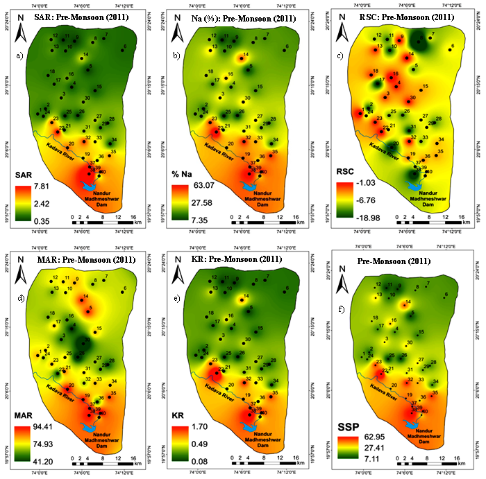
SAR ratio is used to measure the alkali/sodium hazard to the crop and, hence, considered to be an important parameter for determining the water suitability for irrigation because sodium concentration can reduce the soil permeability and soil structure (Todd, 1980). This index gives an idea about the proportion of sodium to calcium and magnesium ions in water. Generally, water having a low SAR value is good for irrigation (Karanth, 1987). SAR values ranges from 0.35 to 7.83 with an average 1.85 (Table 3). As per the Richards (1954) classification (Table 4), all the groundwater samples come under excellent water category for irrigation. The spatial variation map of SAR illustrated that, the Southern regions contain high concentration of sodium. The hotspots (sample numbers 20, 22, 23, 32, 37, 38 and 39) are identified in intense agricultural zone (Figure 5a).
Percent Na is an important ratio used to identify the soluble sodium content of the water and also used to expose the sodium hazard. Sodium by the process of base-exchange replaces calcium in the soil which as result soil permeability reduced (Doneen, 1964). In the study area, the percent Na value ranges from 7.33 to 63.15 with an average 26.26 (Table 3). As per the Doneen classification (Table 4), 45%, 35 % and 17.5% groundwater samples fall in excellent, good and permissible class for irrigation, respectively. However, only one sample (number 22) is characterized as doubtful class of irrigation use. The downstream part of the study area is having intense agriculture, where, high value of Na(%) encountered (Figure 5b).
Generally, water with high concentration of CO3 and HCO3 has the tendency to cause the precipitation of calcium and magnesium as a result water in the soil become concentrated. It leads to relative proportion of sodium (Na+) in the water and, as a result, sodium bicarbonate is increased (Sadashivaiah et al., 2008). When, RSC becomes too high, the CO3 combines with Ca and Mg to form solid material, which settles out of the water and ends with increase in SAR and % Na. Positive RSC shows that sodium built is possible in the soil. The RSC value ranges from -19.00 to -0.98 with an average value of -6.66 (Table 3). According to Richards (1954) classification, RSC value (<1.25) all groundwater samples are considered safe for irrigation (Table 4). The spatial extent map of RSC represented that few hotspots is observed at the North and Central regions of the study area with high RSC value (Figure 5c).
The MAR ratio indicates the excess amount of magnesium (Mg2+) over calcium (Ca2+) (Raghunath, 1987). Generally, the source of magnesium in groundwater is due to ion exchange of minerals from rocks and soils by water (Mukherjee et al., 2005). The high MAR (>50) results in increase soil alkalinity and affects the crop yield. In the study area, a wide range of MAR values are observed with ranges of 40.98 to 94.47 with an average value of 74.87 (Table 3). As per MAR classification, 97.5% samples are unsuitable for irrigation and only 2.5% (number 30) groundwater sample confirm their fitness for irrigation (Table 4). In the vicinity of agricultural areas of south and north regions, where, sample locations like 5, 14, 20, 35, 37, 38 and 39 comprises high MAR value (Figure 5d).
Kelley’s ratio is used to measure the sodium concentration against calcium and magnesium. If ratio is >1 suggests the excessive concentration of sodium which leads to undesirable effects on soil properties and reducing soil permeability. Consequently, water with ratio (>1) is unsuitable and (<1) is supposed to be suitable for irrigation (Kelley, 1951). In this study, KR values ranges from 0.08 to 1.70 with an average 0.41 (Table 3). It is inferred that majority of the groundwater samples (i.e. 95 %) are suitable for irrigation, while 5 % (numbers 19 and 38) are unsuitable for irrigation (Table 4). It is observed that the south part where intense and prolonged agriculture taking place is one of the cause of high concentration of sodium; hence, samples restricted irrigation in downstream part (Figure 5e).
The SSP ratio is used to evaluate sodium hazard. Water with SSP greater than (>60%) may result sodium accumulation; hence, soil physical properties will breakdown. Irrigation with high sodium content water may cause an accumulation of exchangeable sodium ion on soil colloids. Also, continues use of alkaline water for irrigation has adverse effects on soil physical properties and reduces the crop yield (Fipps, 2003). In general, when sodium content is high in irrigation water, sodium ion tends to be absorbed by clay particle, displacing magnesium and calcium ion. The exchange process in soil reduces the soil permeability and affects the internal drainage. The calculated values of SSP varied from 7.09 to 63.03% with an average 25.90% (Table 3). SSP classification suggests that, 45% and 37% groundwater samples fall in good (<20) and permissible (20-40) categories. While, (17.5%), numbers (22, 23, 32, 35, 37, 38 and 39) groundwater samples are come under doubtful category (Table 4). The spatial variation map of SSP illustrated that, high value of SSP is observed in southern part, few patches at central parts of the study area (Figure 5f).
4.3 Multivariate Statistical Analysis
The multivariate statistical analysis was performed to reduce and organize the data with similar hydrochemical characteristics. Total 14 physicochemical parameters were considered for the formulation of Correlation Matrix (CM) and Principle Component Analysis (PCA) and their results are tabulated (Table 5 and 6).
Table 5. Correlation matrix
|
Parameters
|
pH
|
EC
|
TDS
|
TH
|
Ca
|
Mg
|
Na
|
K
|
Cl
|
F
|
CO3
|
HCO3
|
SO4
|
NO3
|
|
pH
|
1
|
|
|
|
|
|
|
|
|
|
|
|
|
|
|
EC
|
-0.16
|
1
|
|
|
|
|
|
|
|
|
|
|
|
|
|
TDS
|
-0.16
|
1.00
|
1
|
|
|
|
|
|
|
|
|
|
|
|
|
TH
|
-0.30
|
0.70
|
0.70
|
1
|
|
|
|
|
|
|
|
|
|
|
|
Ca
|
-0.35
|
0.09
|
0.09
|
0.46
|
1
|
|
|
|
|
|
|
|
|
|
|
Mg
|
-0.22
|
0.75
|
0.75
|
0.96
|
0.20
|
1
|
|
|
|
|
|
|
|
|
|
Na
|
0.12
|
0.77
|
0.77
|
0.50
|
-0.19
|
0.61
|
1
|
|
|
|
|
|
|
|
|
K
|
0.23
|
0.00
|
0.00
|
-0.08
|
-0.03
|
-0.08
|
0.16
|
1
|
|
|
|
|
|
|
|
Cl
|
-0.08
|
0.87
|
0.87
|
0.77
|
0.12
|
0.81
|
0.88
|
0.13
|
1
|
|
|
|
|
|
|
F
|
0.09
|
0.12
|
0.12
|
-0.08
|
-0.38
|
0.03
|
0.24
|
0.36
|
0.12
|
1
|
|
|
|
|
|
CO3
|
-0.20
|
0.16
|
0.16
|
0.45
|
0.16
|
0.44
|
0.19
|
-0.15
|
0.12
|
-0.17
|
1
|
|
|
|
|
HCO3
|
-0.25
|
0.41
|
0.41
|
0.60
|
0.15
|
0.62
|
0.40
|
0.05
|
0.40
|
0.00
|
0.65
|
1
|
|
|
|
SO4
|
-0.20
|
0.63
|
0.63
|
0.66
|
0.25
|
0.65
|
0.37
|
-0.22
|
0.59
|
0.01
|
0.01
|
0.05
|
1
|
|
|
NO3
|
-0.29
|
0.32
|
0.32
|
0.16
|
-0.08
|
0.20
|
0.17
|
-0.08
|
0.20
|
-0.04
|
0.00
|
0.01
|
0.23
|
1
|
Bold values indicates significant correlations among physicochemical parameters.
Table 6. Principal Component Analysis
|
Parameters
|
Factors
|
|
1
|
2
|
3
|
4
|
5
|
|
pH
|
-.013
|
-.226
|
-.419
|
.058
|
-.754
|
|
EC
|
.926
|
.110
|
-.031
|
.051
|
.173
|
|
TDS
|
.926
|
.110
|
-.031
|
.051
|
.173
|
|
TH
|
.768
|
.402
|
.409
|
-.082
|
.087
|
|
Ca
|
.092
|
.075
|
.931
|
-.103
|
.013
|
|
Mg
|
.821
|
.421
|
.156
|
-.058
|
.092
|
|
Na
|
.818
|
.196
|
-.328
|
.203
|
-.093
|
|
K
|
-.010
|
-.023
|
.095
|
.884
|
-.180
|
|
Cl
|
.944
|
.116
|
.038
|
.145
|
-.010
|
|
F
|
.111
|
-.086
|
-.337
|
.696
|
.089
|
|
CO3
|
.084
|
.886
|
.036
|
-.197
|
.018
|
|
HCO0
|
.315
|
.862
|
.078
|
.119
|
.048
|
|
SO4
|
.764
|
-.217
|
.255
|
-.235
|
.154
|
|
NO3
|
.235
|
-.088
|
-.208
|
-.066
|
.791
|
|
Eigenvalues
|
5.945
|
2.165
|
1.532
|
1.124
|
1.003
|
|
Variance (%)
|
42.462
|
15.465
|
10.945
|
8.029
|
7.163
|
|
Cumulative %
|
42.462
|
57.928
|
68.872
|
76.901
|
84.064
|
Bold values indicates the high positive loading.
4.3.1 Correlation Matrix (CM)
The correlation matrix is used to determine the degree of correlation among the various physicochemical parameters which influence groundwater quality in the study area. The correlation analysis involving statistical calculations and gives a measure of how well one parameter predicts the value of another parameter (Pearson, 1896; Kurumbein and Graybill, 1965). In water chemistry, CM is recognized as a common and useful statistical technique to know the positive and negative association of ions (Box et al., 1978; Chapman, 1996). A positive strong correlation can show the same sources of particular ions which can be natural or anthropogenic in origin; while, weak correlation indicates the sources of ions are independent from each other (Islam et al., 2017). The variables showing a correlation coefficient (r>0.7) are considered to be strong; where (r) values between (0.5-0.7) indicate a moderate correlation; while (r < 0.3) is weak correlation. Table 5 illustrated that a positive correlation of EC with TDS (r = 1), Cl (r = 0.87), Mg (r = 0.75), Na (r = 0.77), SO4 (r = 0.63) and TH (r = 0.70) which indicate that the dissolution of salts increases the electrical process of weathering (Wagh et al., 2016a). In case of the study area, the inputs of Mg, Na, TDS, Cl, SO4, and NO3 are influenced by rainfall and human induced activities. Also, the succeeding variables like TDS with TH (r = 0.70), SO4 (r = 0.63), Mg (r = 0.75) and Na (r = 0.77) depicts strong association. Moreover, TH reveal a strong positive relationship with Mg (r = 0.97), SO4 (r = 0.66), Na (r = 0.50) and Cl (r = 0.77). In addition, Mg with Cl (r = 0.81), HCO3 (r = 0.62), Na (r = 61) and SO4 (r = 0.65) shows positive correspondence. It is confirm that Na and Cl have a strong correlation (r = 0.88), Cl and SO4 moderate correlation (r = 0.59), and CO3 with HCO3 (r = 0.63). As well, Ca, Mg, Na and Cl, EC, TH and TDS have confirmed the significant association with irrigation.
4.3.2 Principal Component Analysis (PCA)
It is important to relate the association of different physicochemical parameters and their possible sources of contamination due to complexities of the local hydrogeological conditions and hydrochemical processes that occurs in aquifers which are complicated to explain. Thus, in order to identify the most influencing physicochemical parameters on groundwater quality, R-mode factor analysis using SPSS 22.0v was applied to the hydrochemical data to classify the different groups based on inherent qualities of parameters. R-mode factor analysis examines the relationship among variables by analyzing a matrix of simple correlation coefficients for all pairs of variables considered (Saager and Singlair, 1974). Factor analysis is performed with Kaiser Varimax rotation to differentiate the factors without changing the data structure which helps to reduce the contribution of less significant parameters affecting water quality (Mertler and Vannatta, 2005). Table 6 summarizes the rotated component matrix of five factors with Eigenvalues, % of Variance and Cumulative % of each factor. It is seemed that first factor (Factor 1) accounts for 42.46 % of the total variance and is positively loaded with EC (0.926), TDS (0.926), TH (0.768), Mg (0.821), Na (0.818), Cl (0.944) and SO4 (0.764). The Na and Cl show the highest PC loadings due to their high solubility behavior (Rao, 2014). The high loading of TDS (0.926) is controlled by the Cl, Mg, Na, and SO4 ions; whereas, TH (0.768) is influenced by the correspondence of Mg, Cl and SO4 which indicate the permanent type of water hardness which has been confirmed by a high positive loading with TDS. The high loading of Na over Ca represents the ion exchange process between Ca and Na ion (Drever, 1988). Also, positive loadings of Mg, Na, Cl and SO4 supported that groundwater is significantly influenced by anthropogenic inputs. The Factor 2 shows CO3 (0.886) and HCO3 (0.862) with 15.46% of total variance suggesting groundwater is recharged with fresh water and CO2 dissolution during precipitation and infiltrated water reacts with soil CO2 forming H2CO3. The water with high alkalinity is caused by long-term irrigation practices (Rao, 2014). Therefore, factor 2 is considered to be alkalinity controlled. The third factor (Factor 3) shows high loadings of calcium (0.931) and TH (0.409) with 10.94% of the total variance suggesting a diminutive amount of calcite minerals dissolution. However, Factor 4 is dominated by high loadings of potassium (0.884) and fluoride (0.696) with 8.02% of the total variance owed to the application of fertilizers and agrochemicals in agriculture to increase crop productivity, hence, reflecting anthropogenic origin. The fifth factor (Factor 5) is influenced by nitrate positive loading (0.791) exemplifying the leaching of agricultural and animal wastes, fertilizers and pesticides in the aquifer which turn to increase the concentration of nitrate in the study area.
4.4 Hydrochemical evolution
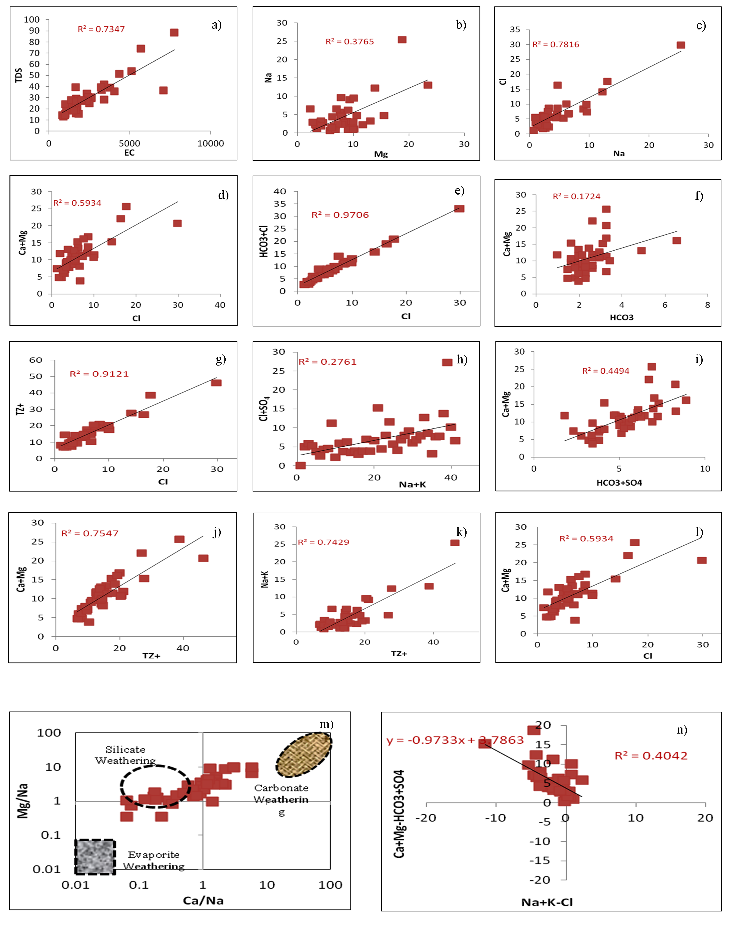
To recognize the hydrochemical evolution within study area, then it is important to know local geology and mineralogical composition of rocks, agricultural inputs, dissolution, precipitation climate condition, etc., influence the groundwater chemistry. In general, during groundwater recharge within aquifer, it reacts with soil, rock-water interactions, types of weathering like silicate or carbonate and significant anthropogenic inputs may alter groundwater composition in the area (Todd, 1980). The scatter plot of EC vs. TDS (Figure 6a) represents good correlation which indicate EC is attributed from dissolution of salts and inorganic pollution load in the water. Scatter plot of Mg vs Na (Figure 6b) represent that weak correlation which confirm that magnesium concentration is increasing due to silicate weathering. The Na/Cl ratio (Figure 6c) is used to identify the salinity mechanism in semi-arid and arid environment (Sarin et al., 1989). The halite maintains the ratio to 1 by releasing Na and Cl ions (Hounslow, 1995). The groundwater ratio of Na/Cl indicates good correlation, if higher value of Na/Cl ratio then the possible source of Na is silicate weathering and; if ratio less than 1 confirm the possibility of ion exchanges of Na with Ca and Mg in clay particles (Tiwari and Singh, 2014).
Cl vs Ca+Mg ratio (Figure 6d) indicates moderate correlation confirmed that the salinity is increased due to chloride is associated with increased contents of Ca + Mg. Na/Cl vs Cl (Figure 6e) illustrated weak correlation due to ion exchange process in groundwater which is adsorb sodium into aquifer in exchange for Ca + Mg (Raju et al., 2016). The plot of Ca+Mg vs HCO3+SO4 (Figure 6e) is used to represent the ion exchange and different weathering processes. 1:1 equiline ratio is maintained by the dissolution of calcite, dolomite and gypsum (Cerling et al., 1989). The significant contribution from silicate weathering and required demand HCO3+SO4 is balanced by alkalis Na+K (Datta et al., 1996). The plot showing positive correlations (r2 = 0.9) indicating ion exchange process is dominant in the groundwater. The ionic concentrations in meq/l are falling above the equiline indicating both carbonate and silicate weathering. Such a plot also shows that HCO3 is in excess of Ca+Mg possibly pointing to the process of ion exchange reaction (Rajmohan and Elango, 2004). The ratio of Ca+Mg/HCO3 (Figure 6f) shows weak correlation. This ratio is significantly used to know the origin of Ca and Mg. If the ratio is less than 0.5 may be due to the depletion of Ca and Mg or weathering minerals like pyroxenes and amphiboles (Sami, 1992). It indicates that alkaline elements (Ca and Mg) may be derived from silicate and carbonate minerals (Mahato et al., 2016). The scatter plot of Cl vs TZ+ (Figure 6g) represents positive correlation (r2 = 0.91) which suggest chloride is enriched due to agricultural waste, excessive use of chemical fertilizers, irrigation water runoff, percolation and leaching of waste, etc. The scatter plot of Na+K vs Cl+SO4 (Figure 6h) depicted that there is increase of alkali elements due to presence of sodium sulphate, potassium sulphate, sodium chloride and potassium chloride in soil system (Bhardwaj et al., 2010). The plot of HCO3 + SO4 vs Ca+Mg indicates that carbonate and silicate weathering is the dominant process (Datta et al., 1996). It is confirm that silicate weathering is the main process followed by carbonate weathering and ion exchange process which are affecting the groundwater quality of the study area (Figure 6i). The plot of total cations (TZ+) vs Ca+Mg illustrated that many of the groundwater samples fall below the equiline and which reflecting high concentration of sodium and potassium with increasing dissolved solids (Figure 6j).
Also, total cations (TZ+) vs Na + K plot (Figure 6k) shows sodium and potassium have positive correlation with total cations particularly at higher concentration. It is illustrated that silicate weathering is dominant process which controls the groundwater chemistry. Scatter plot of Cl vs Ca/Mg (Figure 6L) shows moderate correlation (r2= 0.59) which confirm that salinity is increased due to chloride associated with increase in Ca + Mg and decrease in Na/Cl may be from ion exchange process which adsorbs sodium onto aquifer in calcium and magnesium exchange (Raju et al., 2016). The logarithmic bivariate plot of Mg/Na vs Ca/Na is used to know the type of weathering (Figure 6m). The higher solubility of sodium than calcium which increases the sodium concentration, therefore Ca/Na ratio is expected to low which infers the silicate weathering as dominant geochemical process followed by carbonate weathering due to presence of lime kankar in the area (Zhu et al., 2014). The plot of (Ca+Mg)-(HCO3+SO4) vs (Na+K)-Cl (Figure 6n) confirms cation exchange process. The samples falling close to zero are not affected by ion exchange while those falling on slope line -1 will exchange Na, Ca and Mg ions (Jankowski et al., 1998, Kortatsi, 2006).


 ,
Dipak Panaskar 1
,
Dipak Panaskar 1