Abstract
The study presents an approach to map Land Use / Land Cover Change (LULCC) at large scale and processing techniques that permit higher accuracy. IRS RESOURCESAT-2 LISS-IV images of Nellore district of Andhra Pradesh were used to apply the classification technique. In multi-scale feature extraction approach LULCC takes two forms i.e. conversion from one category of LULCC to another and modification of condition within a category. Thus, major LULCC classes were extracted using object based approach and uncertain classes were identified using onscreen knowledge based method. The results showed in 2009, the accuracy of cropland, water body and built-up segments were 99.3%, 94.79% and 89.72%, respectively, whereas, in 2013 the accuracies were 94.31%, 88.26% and 81.20%, respectively. Hence, this classification approach can be useful in different landscape structure over the time, which can be quantified and assessed to achieve a better understanding of the land cover.
1 . INTRODUCTION
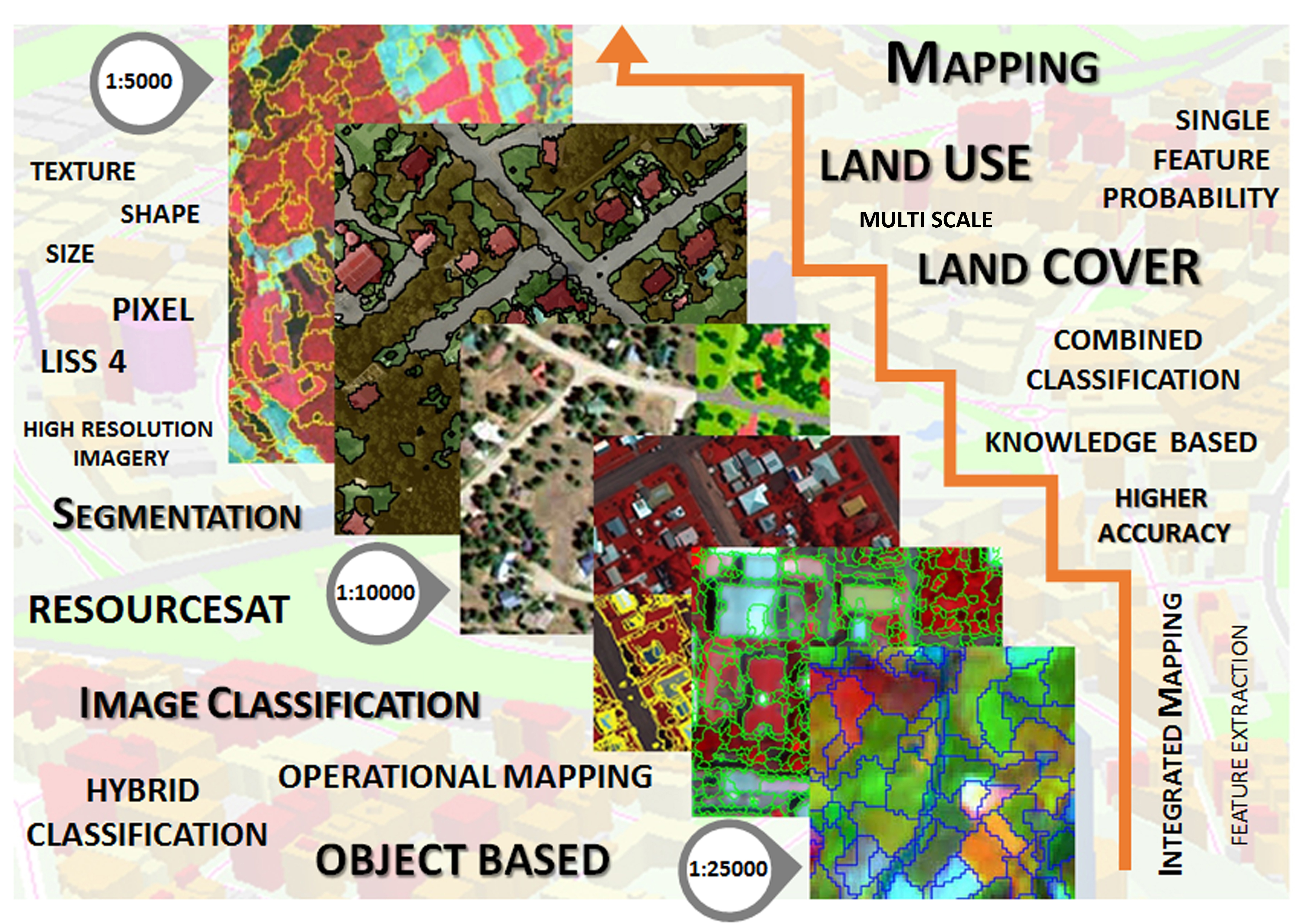
Precise and timely land use / land cover (LULC) information is essential to many government and private organizations at local, regional, national and global levels for different applications such as environmental monitoring and planning, LULC change modeling, transportation planning, urban development planning, urban modeling, etc. Remotely sensed data have been the major sources of prepared LULC maps (Chen and Stow, 2003). For preparing updated LULC information at different scales, remote sensing image classification techniques have been developed since 1980s. During 1980s and 1990s, most classification techniques were employed by keeping image pixel as the basic unit of analysis, in which each pixel is labeled as a single LULC class. Although a large number of remote sensing classification techniques have been developed in recent decades (Lu and Weng, 2007), based on spectral variables; whereas spatial information was more or less ignored. Spectra-based classification approaches are conceptually simple and easy to be implemented, but they neglect the spatial components, which are inherited in real-world remote sensing imagery (Moser et al, 2013). A number of LULC types cannot be effectively separated with spectral information and thereby less than desired accuracy has been reported with spectra-only classifiers (Tso and Mather, 1999; Stuckens et al, 2000). For example, there has been a consensus that impervious surfaces and bare soil (e.g. bright urban impervious surfaces and dry soil, and dark impervious surfaces and moist soil) cannot be effectively separated only with spectral information. These issues become severe with the continued advancements in satellite sensor technologies to capture images at high spatial resolution (i.e. LISS-IV and CARTOSAT-1, 2A, 2B). With higher spatial resolutions, images are likely to have higher within-class spectral variability. As a result, less than satisfactory results have been reached with spectral classifiers (Myint et al, 2011). In remote sensing literature, such approaches have been generally called “spatio-contextual” image classification, indicating the relationship between a “target” pixel and its neighboring pixels is incorporated into analyses (Tso and Mather, 1999). These spatio-contextual image classification approaches can be grouped into three categories, including 1) texture extraction, 2) Markov random fields (MRFs) modeling and 3) image segmentation and object-based image analysis (Stuckens et al, 2000; Blaschke, 2010; Thoonen et al, 2012; Moser et al, 2013). Compared to traditional per-pixel and sub-pixel classification methods, object-based models provide a new paradigm to classify remote sensing imagery (Blaschke, 2010; Myint et al, 2011). As the high spatial resolution images convey more ground information and allow Earth observations with enhanced accuracy of digital information (Aksoy et al. 2010) and thus efficient and accurate extraction of objects from these data is attracting greater attention from remote sensing researchers (Baltsavias, 2004). Hence, object-based approaches are more appropriate for high resolution remote sensing images since they assume that multiple image pixels form a geographic object. So, instead of considering an image as a collection of individual pixels with spectral properties, object-based methods generate image objects through image segmentation (Pal and Bhandari, 1992). Accordingly, object-based image analysis can simultaneously take the spectrum, shape, texture, and semantic relation into the feature space to improve interpretation accuracy (Benz et al 2004; Zhang et al 2013); hence, the use of object-based classification of high resolution image shows a thriving upbeat in innovation of new and novel techniques.
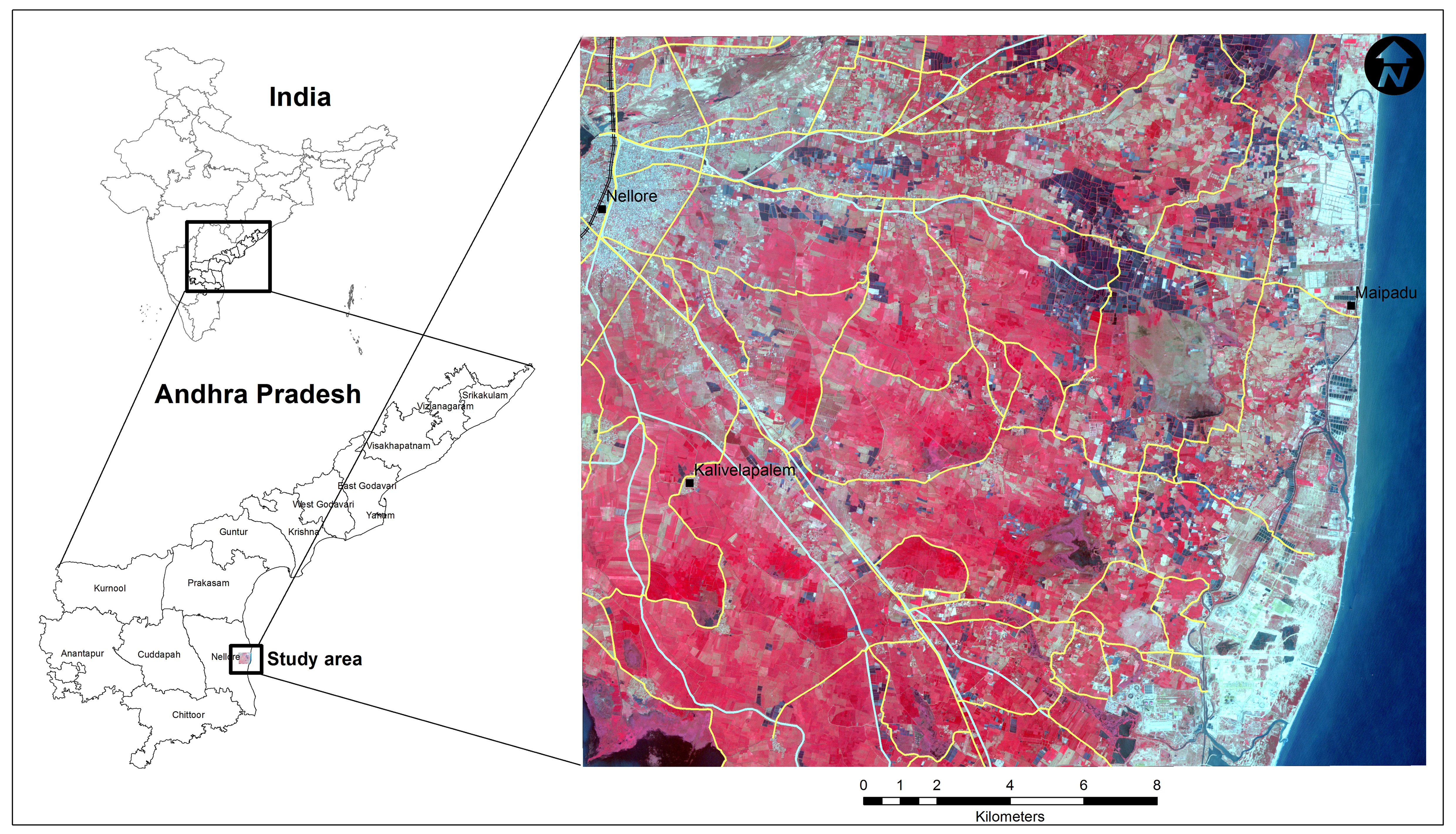
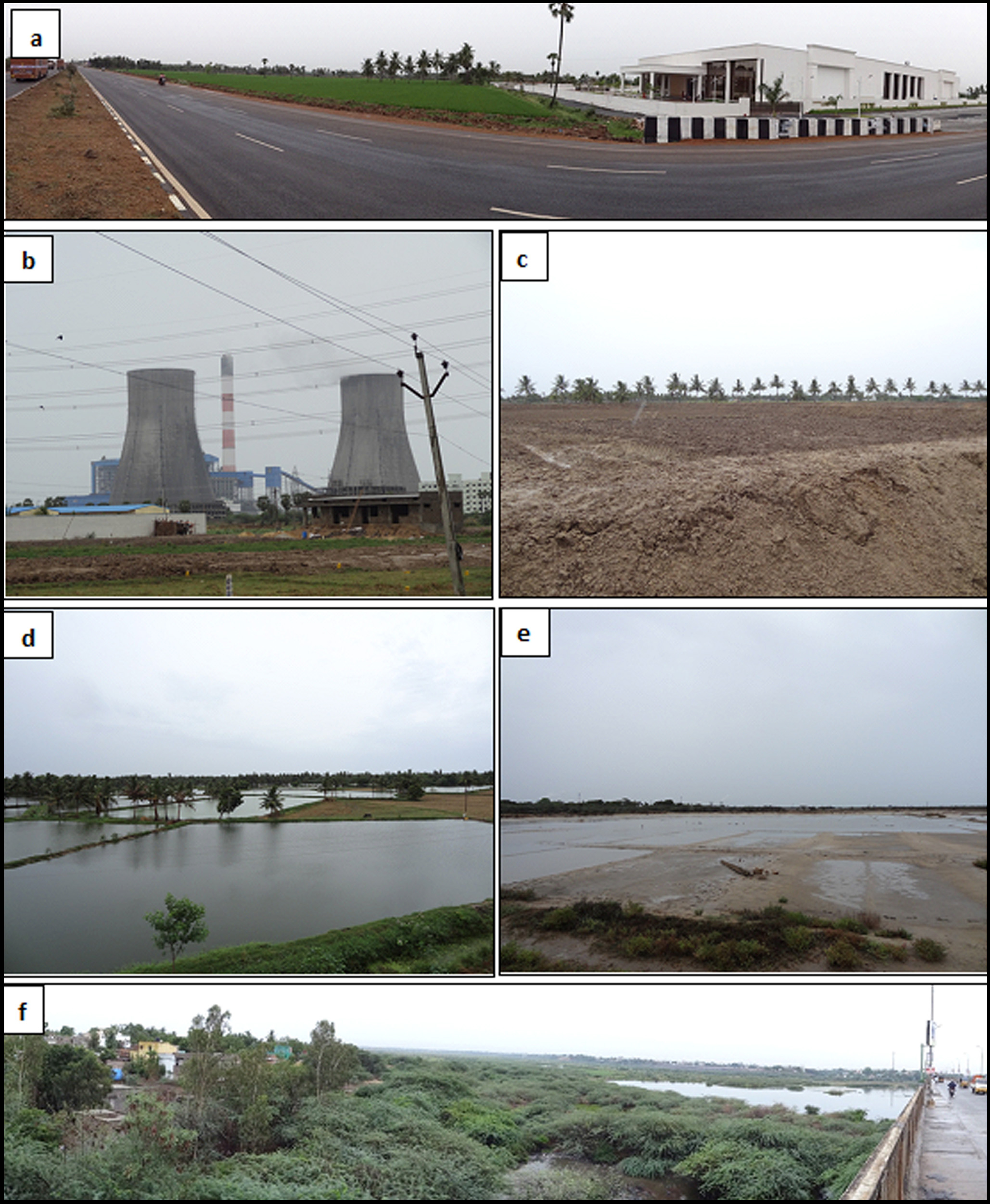
Meaningful objects always exist over a certain range of scales in segmentation of remote-sensing images (Yuan et al, 2014). Hence, to overcome the limitation of the object-based classification an approach has been adopted to enhance the accuracy of the satellite image classification incorporating onscreen modification of post classified image segments. This approach has been taken after observing heterogeneity of the study area, where, built-up areas are with urban, rural, industrial and infrastructure, discriminate water bodies from numerous aqua ponds and partial wetland, discriminate bare lands from vegetated open areas, coastal sand from riverine sand and abandoned aqua ponds. Earlier studies on object-based classification approaches have shown significant higher accuracy (Benz et al, 2004; Wang et al, 2004; Myint et al, 2011). The objective of the present study is to use optimal combinations of object-based and visual LULC classi?cation to obtain higher classi?cation and post-classi?cation change detection accuracies. This hybrid method was applied to IRS RESOURCESAT-2 LISS-IV satellite images of the coastal region of Andhra Pradesh, India. The focus of our study is on LULCC because of rapid industrialization is taking place along the coastal part of this region along with urban expansions.
3 . MATERIALS AND METHODS
3.1 Data Processing
Two cloud-free IRS RESOURCESAT-2 LISS-IV datasets, one from March 22, 2009 and one from March 13, 2013 (WGS 84) with a pixel size of 5.8m x 5.8m were used (Table 1). These images were selected on the basis of their availability and the quality of datasets for the study area. Although different LULC classes for each of the two RESOURCESAT-2 LISS-IV images were conducted separately. Atmospheric correction was also performed.
Table 1. Satellite image specifications
|
Satellite
|
Sensor
|
Dates of pass
|
Spatial resolution
|
Spectral Resolution
|
Radiometric Resolution
|
|
IRS R-2
|
LISS-IV
|
22 March, 2009
|
5.8 m
|
3 bands (2,3,4)
|
8 bit
|
|
13 March, 2013
|
16 bit
|
ERDAS Imagine (2015) was used to process the atmospheric correction of LISS-IV images using the ERDAS Model maker. Image segmentation was performed using eCognition developer 9.0 (2015). Post segmentation rectification and classification accuracy assessment was performed using ArcGIS 10.2.2. Thirteen level-2 LULC classes were selected for the classi?cation process of 2009 and 2013 datasets following the classification scheme of NRSC (2011) (Table 2).
Table 2. Land use / land cover classification schemes (NRSC, 2011)
|
Level 1 classes
|
Level 2 classes
|
LUCODE
|
Description
|
|
Built up
|
Compact
|
1
|
All places with a municipality, corporation or cantonment or notified town.
|
|
Sparse
|
2
|
Areas where discrete uses are not distinguishable or separable.
|
|
Vegetated/open area
|
3
|
Includes vegetation cover midst urban areas, play grounds, stadium, racecourse, golf course, gardens, parks, zoo, beaches and skiing areas.
|
|
Rural
|
4
|
Built up areas smaller in size, mainly associated with agriculture and allied sectors and non-commercial activities.
|
|
Industrial
|
5
|
Human activity is observed in the form of manufacturing along with other supporting establishments of maintenance. Heavy metallurgical industry and thermal cement, petrochemical, engineering plants.
|
|
Agriculture
|
Cropland
|
6
|
Areas with standing crop as on the date of satellite overpass. It appears bright red to red in color with varying shape and size in a contiguous to non-contiguous pattern.
|
|
Fallow land
|
7
|
Cropland areas, which are uncropped during the agricultural year under consideration as on the date of satellite overpass during all cropping seasons.
|
|
Plantation
|
8
|
Includes tea, coffee and rubber, which are normally grown in the hilly regions and closely associated with forest cover.
|
|
Aquaculture
|
9
|
Located mostly along the coast or in lakes, river and estuaries where fish are bred and reared for commercial purposes.
|
|
Wasteland
|
Scrub land
|
13
|
The land which is generally prone to deterioration due to erosion.
|
|
Sandy
|
15
|
Areas that have stabilized accumulation of sand, in coastal, riverine or inland areas.
|
|
Wetland
|
Wetland
|
16
|
All submerged or water saturated lands, natural or man-made, inland or coastal, permanent or temporary, vegetated or non-vegetated, which necessarily have a land-water interface.
|
|
Water body
|
Water body
|
17
|
Surface water in the form of rivers, canals, ponds, lakes and reservoirs.
|
3.2 Ground Validation
The locations of these training sites were captured using GPS enabled geotagged camera. Additional training samples for each land cover class (190 in total) were derived from high resolution imagery available in Bhuvan Geo-portal (Bhuvan, 2016). The training samples were used as inputs for the classi?cation analysis and accuracy assessment.
3.3 Image Classification
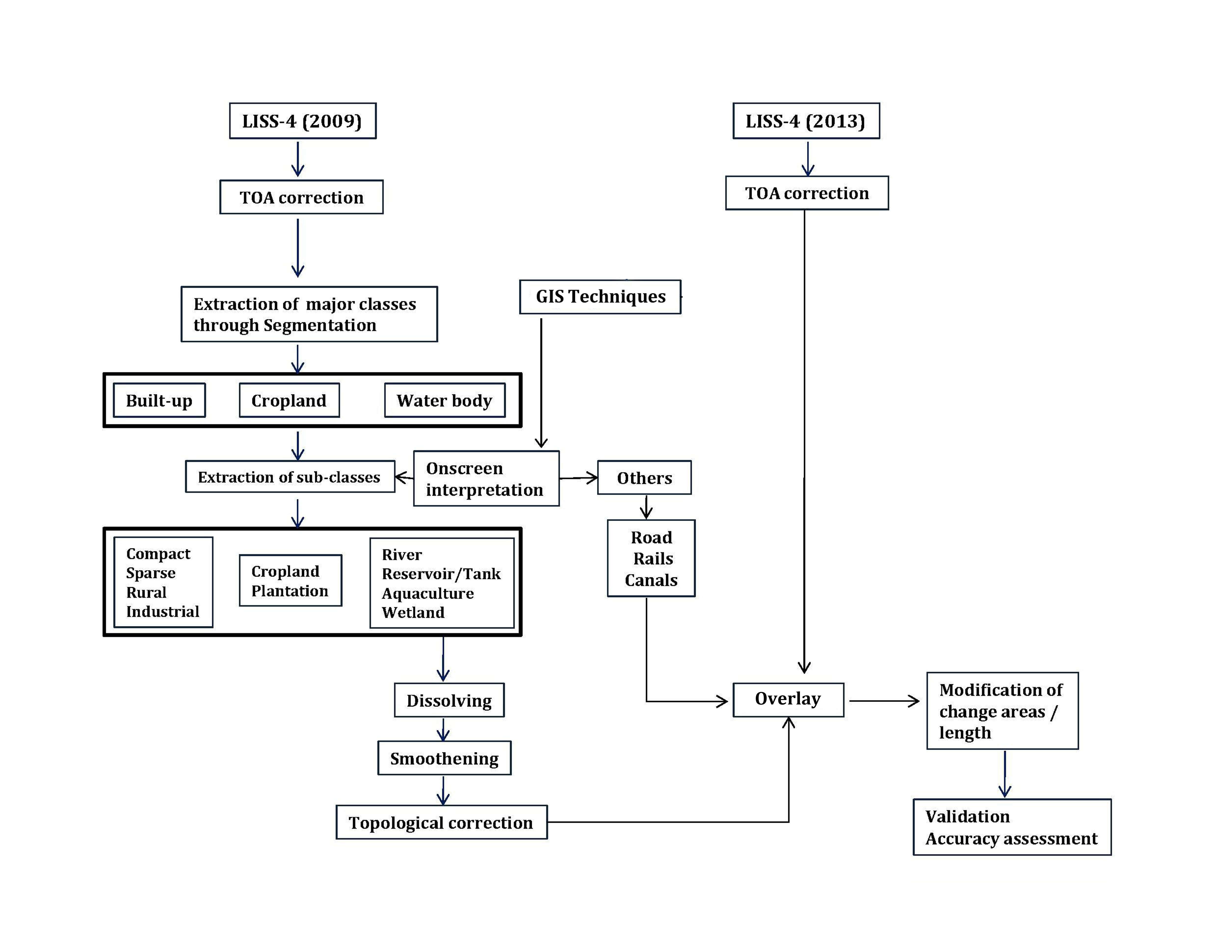
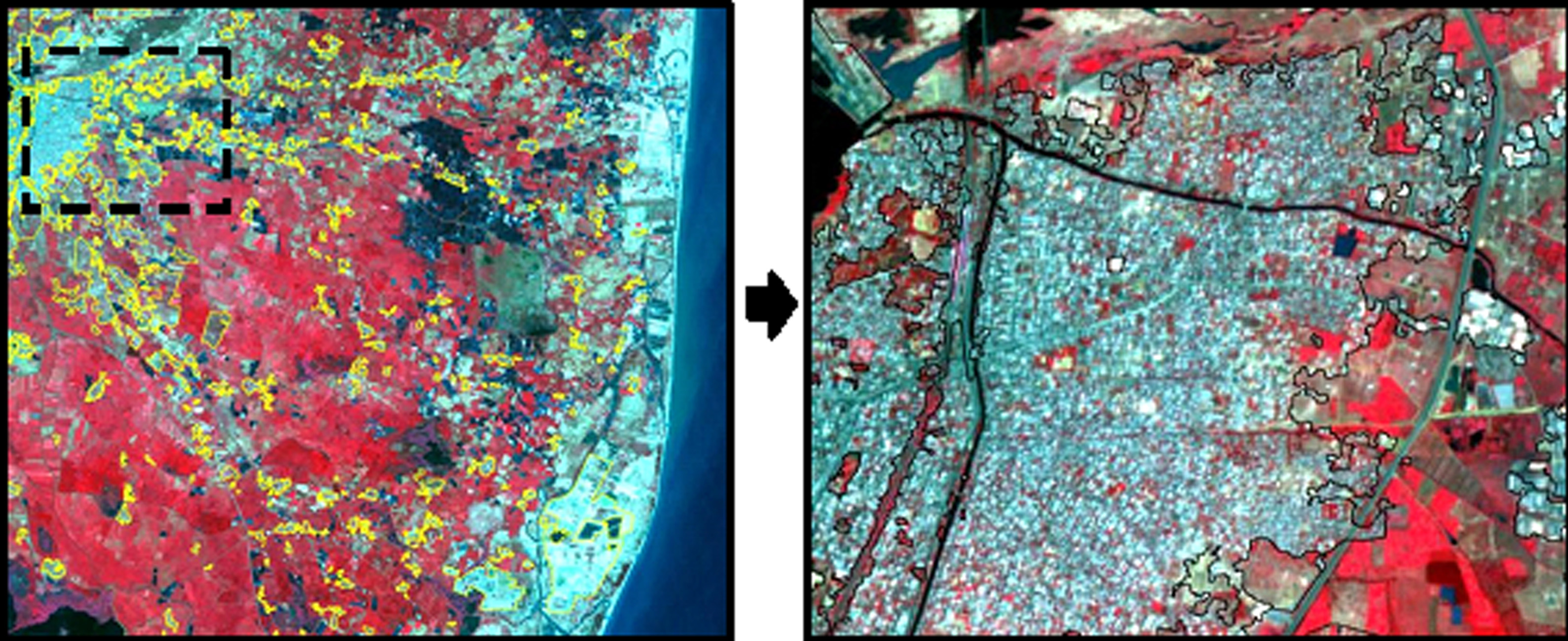
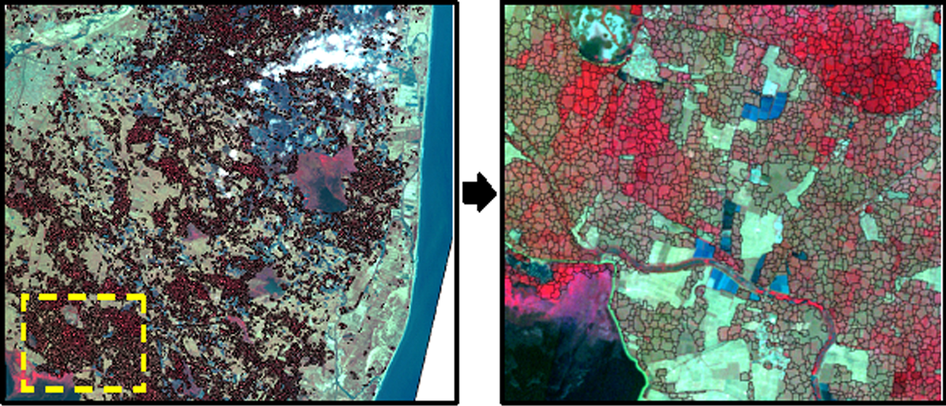
The steps for preparing a LULC map that includes the combination of the object-based and onscreen LULC classi?cation is presented in the map (Figure 2). In the object-based classi?cation method, the LISS-IV images were segmented into image objects. This segmentation process creates image objects that re?ect group of spatially homogeneous neighboring pixels are iteratively clustered until a preset threshold is exceeded. If more weight is assigned to particular spectral layers, these layers have more in?uence on the resulting segmentation boundaries. The parameters used during the segmentation process are scale, shape and compactness. The scale parameter determines the maximum size of the created object, the shape factor controls for the spectral information and shape, and the compactness factor determines compactness of the objects’ edges/borders (Definiens, 2010). In the present study merging technique has been successfully applied on satellite images to extract the major LULC classes. In this study a visual resemblance to potential objects were recognized following a ‘trial and error’ approach (Im et al. 2008; Robertson and King, 2011). Hence, major LULC classes like built-up, cropland and water bodies were clipped out separately from the segmented layers to avoid redundancy (Figure 2).
In this study, to bring out a satisfactory visual match between image objects and landscape features, the segmentation parameters (scale- 5, shape- 0.1 and compactness- 0.5; a weight of 2 for the infra-red layer) were selected on the basis of assigned value of Gutiérrez et al. (2012), which proved satisfactory during ?eld visits in the summer of 2015.
3.4 Segmentation and Overlay
Segmentation was performed on LISS-IV image of 2009. After segmentation, output layers were used for onscreen modification and extraction of sub-classes using ArcGIS software. Advantage of updating and converting level-1 segments into level-2 sub-classes using onscreen value addition lies in its simplicity and error less interpretation. All the value added data was bring into one database using union method. It has also been noticed that the union layer has increased the no of features, which were further dissolved according to classes and to reduce feature number. Slivers were also eliminated through merging with adjacent bigger polygons. To remove the staircase geometric shape of the segments using 25m smoothening process was implied and finalized through topological correction. In the next step of image classification we have used the total classified vector dataset of 2009 and overlaid on 2013 satellite image to identify the LULC changes using onscreen interpretation (Roy et al, 2015). Thus, same dataset of 2009 has been updated with additional field contained 2013 LULC classes. Accuracy assessment reports for individual class categories and overall classi?cation accuracies were performed for classified image of 2013.
3.5 Change Detection
A multi-date post classification comparison change detection technique was used to determine changes in LULC between 2009 and 2013. This is perhaps the most common approach to change detection (Jensen, 2004) and has been successfully used by NRSC (2011) to monitor LULC changes at 1: 50000 scale for entire India. The post-classification approach provides ‘From–To” change information and the kind of landscape transformations that can be easily calculated and mapped (Yuan et al, 2005). A change detection map with 62 combinations of ‘From-To’ change information were derived from prepared for 2009 and 2013.
3.6 Classification and Change Detection Accuracy Assessment
Assessments of the classi?cation accuracy of the LULC maps were conducted by comparing samples of the classi?ed layer and reference layer following Congalton (1991). Fifty reference points were veri?ed by ?eld visits, and 190 reference points were veri?ed through comparison with recent Bhuvan imagery dated between 2009 and 2014 (Bhuvan, 2016). The class and overall accuracies, which provide an indication of the classi?cation agreement between two maps (the classi?ed and the ground-truth maps) that is not attributable to chance, were calculated and are presented as error matrices. The change detection accuracy was obtained by random sampling method to calculate an error matrix for obtained classes (Fuller et al, 2003; Yuan et al, 2005). Classification of the polygons as ‘change’ and ‘no change’ in the resulting LULC change layer was conducted. A total of 24282 polygons were used in the change detection assessment: 12748 polygons for the ‘change’ and 11534 for the ‘no change’ category. All reference polygons were validated through ?eld visits and an inspection of Bhuvan imagery.
4 . RESULTS AND DISCUSSIONS
4.1 Segmentation Accuracy
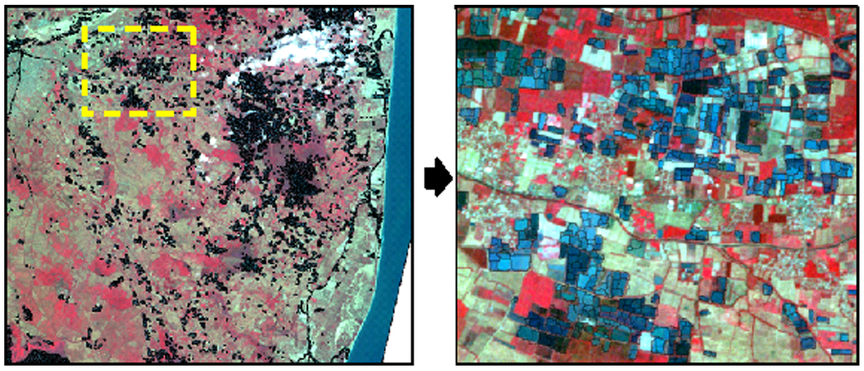
Extraction of major LULC dominant classes separately through segmentation shows higher accuracy to identify objects with homogenous spectral and textural characteristics. In the present study, the built-up, cropland and water body were having higher dominance over the study area (Saxena et al, 2014) hence, were segmented separately (Figures 3, 4 and 5). The results of the segmentation accuracy are presented in table (Table 3). The accuracy assessments with respect to the post classified segments of 2009 show overall accuracy of cropland, water body and built-up segments were 99.3%, 94.79% and 89.72%, respectively.
Table 3. Accuracy assessment for segmentation
|
Segments
|
Accuracy
|
|
Built-up
|
89.72%
|
|
Cropland
|
99.30%
|
|
Water body
|
94.79%
|
It was noticed from the accuracy of the built-up segment that due to complexity of LULC of the study area (Lu and Weng, 2007), it has achieved a comparatively less than water body and cropland. More specifically the presence of abandoned aqua ponds and adjacent built-up areas have created similar textural and spectral identity which were reduced the efficiency to extract segments precisely.
4.2 Modification and Extraction of Sub-Classes
Extraction of major LULC classes and many sub-classes cannot be depicted either object based or pixel based method. Thus, through onscreen value addition to the extracted segmented layer, thirteen level-2 classes were brought out. Table (Table 4) shows total number of segments was classified at level-1, which were further sub-divided into thirteen LULC classes at level-2.
Table 4. Modification of extracted segments at level-2
|
Level-1
|
Level-2
|
Segments
|
Total
|
Extraction type
|
|
Built-up
|
Compact
|
129
|
559
|
Automatic
|
|
Sparse
|
67
|
Value addition to compact
|
|
Vegetated
|
94
|
Value addition to compact
|
|
Rural
|
210
|
Value addition to compact
|
|
Industrial
|
59
|
Value addition to compact
|
|
Agriculture
|
Cropland
|
2532
|
5238
|
Automatic
|
|
Fallow land
|
814
|
Manually
|
|
Plantation
|
126
|
Value addition to cropland
|
|
Aquaculture
|
1766
|
Value addition to water body
|
|
Wasteland
|
Scrubland
|
425
|
428
|
Manually
|
|
Sandy area
|
3
|
Value addition to built-up
|
|
Wetland
|
Wetland
|
62
|
62
|
Value addition to water body
|
|
Water body
|
Water body
|
203
|
203
|
Automatic
|
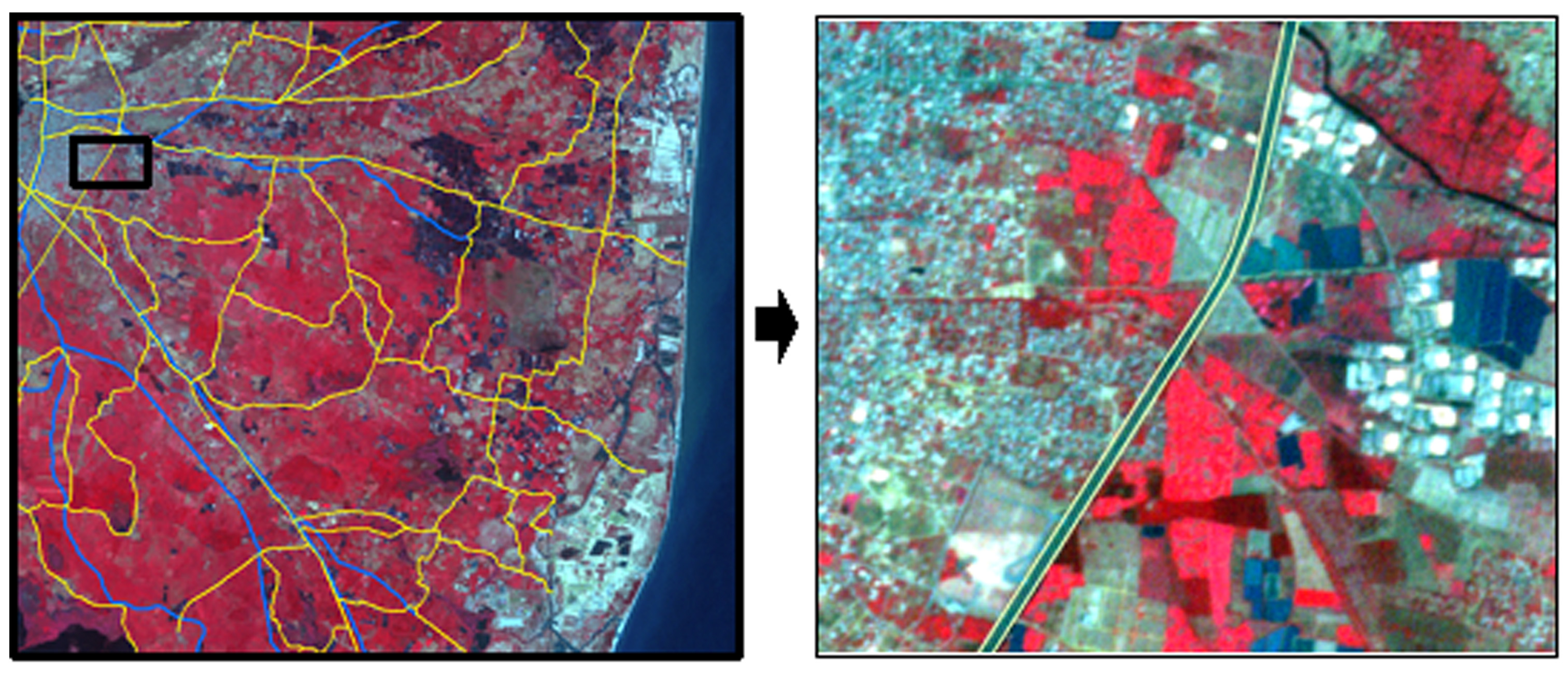
It has also been noticed from the LISS-IV satellite image that, the study area is covered by few irrigation canal which is covering an area about 2.9 sq. km. Similarly, the study area is covered by few major roads and rails which are covering an area about 0.73sq.km. These segments have been extracted onscreen to incorporate in LULC mapping (Figure 6 and Table 5).
Table 5. Modification of extracted segments at level-2
|
Type
|
Mappable No.
|
Length (km)
|
Area coverage (km2)
|
|
Roads
|
2
|
4
|
0.73
|
|
Canals
|
8
|
104
|
2.9
|
4.3 Classification Accuracy
The overall accuracy achieved for the LULC map shows the capabilities of combined classification approach. The Kappa statistic (0.89) also shows a good classi?cation agreement. Kappa values were 0.88 for combined method, showing that the classi?cation agreement between images ranged from good to very good (Monserud and Leemans, 1992). A ‘From-To’ change analysis in the present study introduced more accurate results applying a combined classi?cation approach, delivering greater insight into actual and LULC change increase in ‘urban’, ‘agriculture’, ‘aquaculture’ and ‘industrial’ areas. The results of the classi?cation accuracy assessment showed in table (Table 6). These results show that the extraction and merging of the best- classi?ed classes from object-based and onscreen methods produces a LULC map with improved accuracy in comparison to individual object-based or pixel based classi?cation methods.
Table 6. Classification accuracy for 2013
|
Level-1
|
Level-2
|
User's accuracy
|
Producer's accuracy
|
|
Built-up
|
Compact
|
0.96
|
0.96
|
|
Sparse
|
0.80
|
0.89
|
|
Vegetated
|
0.83
|
0.86
|
|
Rural
|
0.93
|
0.95
|
|
Industry
|
0.92
|
0.95
|
|
Agriculture
|
Cropland
|
0.88
|
0.91
|
|
Fallow land
|
0.91
|
0.83
|
|
Plantation
|
0.89
|
0.91
|
|
Aquaculture
|
0.95
|
0.96
|
|
Wasteland
|
Scrubland
|
0.80
|
0.84
|
|
Wetland
|
Wetland
|
0.89
|
0.94
|
|
Water body
|
Water body
|
0.84
|
0.86
|
|
Overall accuracy
|
0.89
|
|
Kappa statistic
|
0.88
|
4.4 Land Use / Land Cover Change
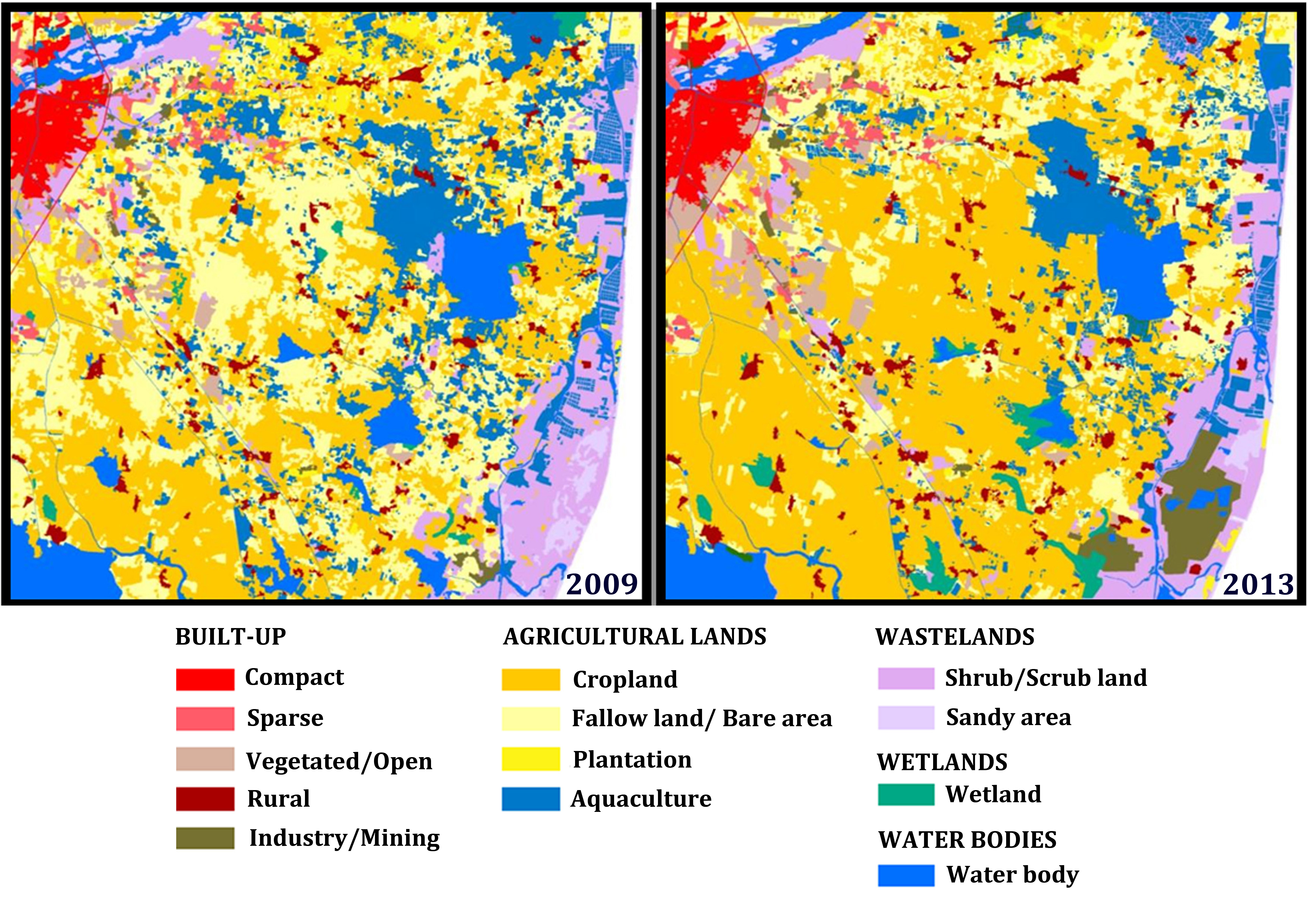
It has been observed (Figure 7) in comparing both the classification output that there has been a major transformation from scrubland to industrial expansion along the coast of study area. The map also depicted the major transformation of aquaculture to agriculture during 2009-2013. A total of 61 possible LULC changes were detected (Table 7), of which 24 are larger than 1 km2. Most of LULC changes are the result of agriculture intensification, industrialization and urban expansion.
Table 7. Land use / land cover change combinations and converted area
|
No.
|
‘From – To’ Classes
|
Area (sq.km)
|
No.
|
‘From – To’ Classes
|
Area (sq.km)
|
|
1
|
Aquaculture to Cropland
|
14.19
|
32
|
Plantation to Built-up Industries
|
0.04
|
|
2
|
Aquaculture to Fallow land
|
9.44
|
33
|
Plantation to Built-up Rural
|
0.13
|
|
3
|
Aquaculture to Built-up Industries
|
0.98
|
34
|
Plantation to Built-up Vegetated
|
0.15
|
|
4
|
Aquaculture to Built-up Rural
|
0.2
|
35
|
Plantation to Wasteland-Scrubland
|
0.36
|
|
5
|
Aquaculture to Built-up Vegetated
|
0.81
|
36
|
Built-up Vegetated to Built-up Compact
|
0.27
|
|
6
|
Aquaculture to Wasteland-Scrubland
|
3.02
|
37
|
Built-up Vegetated to Built-up Sparse
|
0.18
|
|
7
|
Aquaculture to Water body
|
0.27
|
38
|
Wasteland Sandy to Aquaculture
|
0.13
|
|
8
|
Aquaculture to Wetland
|
0.12
|
39
|
Wasteland Sandy to Fallow land
|
0.09
|
|
9
|
Cropland to Aquaculture
|
2.68
|
40
|
Wasteland Sandy to Agri. Plantation
|
0.09
|
|
10
|
Cropland to Fallow land
|
20.11
|
41
|
Wasteland Sandy to Built-up Industries
|
0.94
|
|
11
|
Cropland to Agri. Plantation
|
2.03
|
42
|
Wasteland Sandy to Built-up Sparse
|
0.04
|
|
12
|
Cropland to Built-up Compact
|
0.16
|
43
|
Wasteland Sandy to Wasteland-Scrubland
|
1.52
|
|
13
|
Cropland to Built-up Industries
|
0.55
|
44
|
Wasteland Sandy to Water body
|
1.11
|
|
14
|
Cropland to Built-up Rural
|
1.64
|
45
|
Wasteland Scrubland to Aquaculture
|
2.34
|
|
15
|
Cropland to Built-up Sparse
|
0.27
|
46
|
Wasteland Scrubland to Plantation
|
0.58
|
|
16
|
Cropland to Built-up Vegetated
|
2.2
|
47
|
Wasteland Scrubland to Built-up Compact
|
0.35
|
|
17
|
Cropland to Wasteland-Scrubland
|
2.8
|
48
|
Wasteland Scrubland to Built-up Industries
|
5.3
|
|
18
|
Cropland to Water body
|
0.47
|
49
|
Wasteland Scrubland to Built-up Rural
|
0.54
|
|
19
|
Cropland to Wetland
|
1.23
|
50
|
Wasteland Scrubland to Built-up Sparse
|
0.15
|
|
20
|
Fallow land to Aquaculture
|
3.7
|
51
|
Wasteland Scrubland to Built-up Vegetated
|
1.97
|
|
21
|
Fallow land to Cropland
|
68.54
|
52
|
Wasteland Scrubland to Wasteland Sandy
|
0.91
|
|
22
|
Fallow land to Agri. Plantation
|
0.98
|
53
|
Wasteland Scrubland to Water body
|
1.28
|
|
23
|
Fallow land to Built-up Compact
|
0.08
|
54
|
Wasteland Scrubland to Wetland
|
0.13
|
|
24
|
Fallow land to Built-up Industries
|
0.93
|
55
|
Water body to Cropland
|
0.87
|
|
25
|
Fallow land to Built-up Rural
|
0.83
|
56
|
Water body to Fallow land
|
0.46
|
|
26
|
Fallow land to Built-up Sparse
|
0.36
|
57
|
Water body to Wasteland-Sandy
|
1.32
|
|
27
|
Fallow land to Built-up Vegetated
|
2.74
|
58
|
Water body to Wetland
|
4.1
|
|
28
|
Fallow land to Wasteland-Scrubland
|
3.06
|
59
|
Wetland to Cropland
|
0.66
|
|
29
|
Fallow land to Water body
|
0.2
|
60
|
Wetland to Fallow land
|
0.52
|
|
30
|
Plantation to Cropland
|
1.54
|
61
|
Wetland to Water body
|
0.48
|
|
31
|
Plantation to Plantation
|
1.25
|
|
|
|
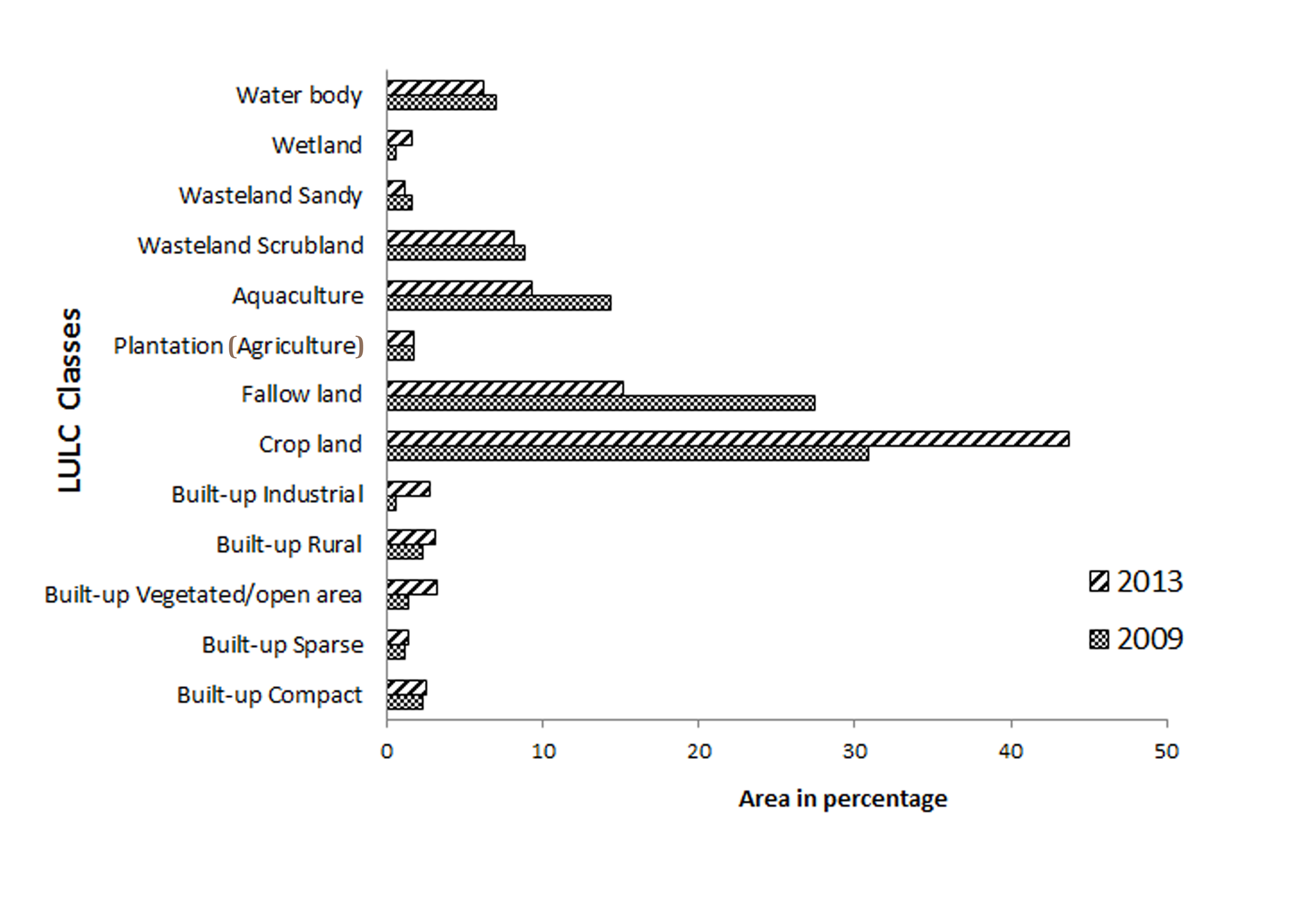
A summary of the LULC change results is provided in table (Table 8). Approximately 230 km2 (56.9%) of the total study area (404.46 km2) remained unchanged, and 174.46 km2 (43.1%) changed. LULC classes, viz. cropland, scrubland, aquaculture and industry are more dynamic in nature (Table 7). Hence, all the classes have major contribution in 2013 LULC change. The study investigated that there was a considerable increase of cropland, industry and built-up vegetated area by 12.78 %, 2.16% and 1.83%, respectively in 2013. Simultaneously, decrease in fallow land, aquaculture and scrubland by 12.25%, 4.99% and 0.69%, respectively in 2013 has also been observed (Table 8). It has been noticed that, ‘Aquaculture’ class was lost between 2009 and 2013 and mostly transformed into ‘cropland’ and ‘urban built-up vegetated’ (Table 9). It has found that majority of the urbanization primarily occurred in the cropland areas (Tian et al, 2014). ‘Industrial’ area replaced almost 8.74 km2 of scrubland, cropland, fallow land and aquaculture in total, which is an increase of 2.16% of TGA. The ‘Urban’ class replaced nearly 9.29 km2 of the ‘cropland’ and ‘fallow land’ and ‘scrubland’ class which is 2.29 % of TGA.
Table 8. LULC change statistics for 2009 and 2013
|
Level-1 Classes
|
Level-2
Classes
|
Area in sq. km
|
Change (%) w.r.t TGA
|
|
2009
|
2013
|
Change
|
|
Built up
|
Compact
|
9.12
|
9.97
|
0.86
|
0.21
|
|
Sparse
|
4.64
|
5.65
|
1.01
|
0.25
|
|
Vegetated/open area
|
5.57
|
12.99
|
7.42
|
1.83
|
|
Rural
|
9.36
|
12.71
|
3.35
|
0.83
|
|
Industrial
|
2.34
|
11.08
|
8.74
|
2.16
|
|
Agriculture
|
Crop land
|
125.06
|
176.74
|
51.68
|
12.78
|
|
Fallow land
|
110.9
|
61.34
|
-49.56
|
-12.25
|
|
Plantation
|
6.96
|
7.17
|
0.21
|
0.05
|
|
Aquaculture
|
57.93
|
37.74
|
-20.19
|
-4.99
|
|
Wasteland
|
Scrubland
|
35.51
|
32.71
|
-2.8
|
-0.69
|
|
Sandy area
|
6.41
|
4.7
|
-1.71
|
-0.42
|
|
Wetland
|
Wetland
|
2.46
|
6.39
|
3.94
|
0.97
|
|
Water body
|
Water body
|
28.21
|
25.27
|
-2.95
|
-0.73
|
Table 9. LULC change matrix (2009-2013)
|
Land Use / Land Cover- 2009
|
Land Use / Land Cover- 2013
|
|
LU Codes
|
1
|
2
|
3
|
4
|
5
|
6
|
7
|
8
|
9
|
13
|
15
|
16
|
17
|
2009 Total
|
|
1
|
9.12
|
|
|
|
|
|
|
|
|
|
|
|
|
9.12
|
|
2
|
|
4.64
|
|
|
|
|
|
|
|
|
|
|
|
4.64
|
|
3
|
0.27
|
0.18
|
5.11
|
|
|
|
|
|
|
|
|
|
|
5.57
|
|
4
|
|
|
|
9.36
|
|
|
|
|
|
|
|
|
|
9.36
|
|
5
|
|
|
|
|
2.34
|
|
|
|
|
|
|
|
|
2.34
|
|
6
|
0.16
|
0.27
|
2.2
|
1.64
|
0.55
|
90.92
|
20.11
|
2.03
|
2.68
|
2.8
|
|
1.23
|
0.47
|
125
|
|
7
|
0.08
|
0.36
|
2.74
|
0.83
|
0.93
|
68.54
|
29.48
|
0.98
|
3.7
|
3.06
|
|
|
0.2
|
111
|
|
8
|
|
|
0.15
|
0.13
|
0.04
|
1.54
|
1.25
|
3.48
|
|
0.36
|
|
|
|
6.96
|
|
9
|
|
|
0.81
|
0.2
|
0.98
|
14.19
|
9.44
|
|
28.89
|
3.02
|
|
0.12
|
0.27
|
57.9
|
|
13
|
0.35
|
0.15
|
1.97
|
0.54
|
5.3
|
|
|
0.58
|
2.34
|
21.97
|
0.91
|
0.13
|
1.28
|
35.5
|
|
15
|
|
0.04
|
|
|
0.94
|
0.01
|
0.09
|
0.09
|
0.13
|
1.52
|
2.47
|
0.01
|
1.11
|
6.41
|
|
16
|
|
|
|
|
|
0.66
|
0.52
|
|
|
|
|
0.8
|
0.48
|
2.46
|
|
17
|
|
|
|
|
|
0.87
|
0.46
|
|
|
|
1.32
|
4.1
|
21.46
|
28.2
|
|
2013 Total
|
9.97
|
5.65
|
12.99
|
12.70
|
11.10
|
176.70
|
61.34
|
7.17
|
37.70
|
32.70
|
4.70
|
6.39
|
25.30
|
404
|
The classified map is showing that there was a substantial interclass change about 12% of TGA between cropland and fallow land, but it was found as not considerable due to unavailability of multi season data. The most striking ?ndings were that the largest patch of aquaculture field and scrub land has been decreased to approximately 12 km2 due to industrial development after 2011 along the coastal track (Figure 8 and Figure 9).
An objective of the study was to establish a method for mapping LULC that can be applied at large scale mapping. We were interested to develop a methodology to classify high resolution satellite image with maximum accuracy. We performed a combined object based and onscreen classification techniques together. The combined classi?cation approach has the advantage that only classes with the highest classi?cation accuracies contribute to the ?nal LULC map, resulting in a higher overall classi?cation accuracy (Gutiérrez et al, 2012). Other authors have also obtained higher classi?cation accuracies when applying a combination of classi?cation methods, including Bhaskaran, Paramananda and Ramnarayan (2010). Minimal errors introduced during classification of imagery can be overcome by applying query based onscreen rectification. We were used the same database to update the change using satellite image of 2013, hence, it did not require further topological correction and simultaneously it reduces the classification error .
5 . CONCLUSIONS
Object and onscreen based classification present a promising mode to improve classi?cation of remotely sensed images. Discrimination of LULC classes with different spectral, textural, and topographical characteristics using combined object-based and onscreen classi?cation approaches may lead to advance work?ows for classifying past, present and future LULC. This technique is very useful for a complex LULC, where LULC class change rate is very high. As the accuracy for the present study is very high, so we recommend this classification approach for region with different characteristics. However, significance research is still required to reduce the subjectivity and human bias of onscreen rectification procedure.
Operational GIS projects related to LULC needs highly accurate datasets on timely basis, which can further be integrated with other datasets during decision making processes. The classification approaches in this study have produced highly accurate datasets which can be maintained and updated within GIS environment. Furthermore, it will be bene?cial for researchers and decision makers to execute the development plan for certain LULC.


 ,
Mohit Modi 1
,
Mohit Modi 1