Keywords

divergence , land use land cover , radar , optical , Remote Sensing

1 . INTRODUCTION

The growth and advancement of remote sensing sensors, platforms, and related technologies (e.g. Geographic Information Systems and Global Positioning Systems) have revolutionized the way in which geospatial data about the Earth’s surface has been collected (Toth and Jóźków, 2016). Such data provides a critical basis for many applications, which use this data to make important decisions that impact the health and well-being of society. The mapping of land use and land cover (LULC) is one such important application. These changes can range from small localized events (e.g. the building of a new residential neighborhood) to that of changes that have much more profound impact (e.g. large-scale deforestation). Quite often they are in response to the need to meet the demands of the growing global population (e.g. the provision of food, water, and shelter), which is currently estimated to be 7.6 billion and is expected to increase to 9.7 billion by 2050 (United Nations, 2019). Meeting the needs of this growing population is no easy feat, and will continue to rely on up-to-date LULC information derived from remote sensing systems to support sustainable planning initiatives (Nath, 2018).

Traditionally, LULC was extracted primarily from optical sensors, such as those on board the Landsat spaceborne missions. These sensors, however, have several drawbacks for collecting LULC information including their inability to penetrate atmospheric disturbances, and they are fully dependent on the Sun’s energy to be functional (Aghababaee et al., 2013; Reiche et al., 2015; Mishra et al., 2017). The use of radar sensors overcome these challenges, providing a valuable tool for collecting LULC data in those regions of the world where those conditions persistent. Several studies have also examined the fusion of both optical and radar data for extracting LULC information, showing higher mapping accuracies compared to the use of each data type on its own (e.g. Pereira et al., 2013; Idol et al., 2015a, Symeonakis et al., 2018). Moreover, within the last decade there has been an increase in the number of free and accessible sources of optical and radar data from different platforms; this has provided many new opportunities for advancing LULC research.

The increasing amount of available remote sensing data has provided many new opportunities for overcoming data gaps in LULC mapping, especially in developing countries (for example, see a recent review of LULC mapping globally by Joshi et al., 2016). However, working with such large volumes of data is not without its own challenges. One such challenge is how to sieve through and select the most relevant image bands for mapping and monitoring LULC, and for specific areas. Generally, as more image bands of data are added, this leads to an increase in classification accuracy since the probability of spectral separability between LULC classes is also increased. However, there is no guarantee that all image bands will be of value in the classification process. Some image bands with similar wavelengths may also be correlated with each other (Sinduja et al., 2015); this can increase processing time, which may be substantial when using some machine learning algorithms to classify imagery (Catak and Babalan, 2013). Likewise, many algorithms used to extract features from imagery may become intractable when tasked with the processing of high dimensional data, thus rendering their use for real world applications inapplicable (Liu, 2015). To accommodate the increased number of image bands, the size of the training samples must also be increased, however such growth is exponential, an issue known as the Hughes phenomenon (Hughes, 1968). Failure to increase the size of training samples accordingly while increasing the number of image bands will typically lead to an initial continual increase in classification accuracy up to a peak point. Following this, the accuracy begins to decrease (Haack and Mahabir, 2017).

Other factors can also impact the properties of the accuracy curve (e.g. rate of decrease, peak accuracy, and shape), all of which ultimately influence the selection of the optimum number of image bands needed for a viable LULC classification. Major factors include the choice of remote sensing classifier, the properties of the image bands being evaluated, and the ability of these image bands to discriminate between the different LULC classes being examined. With respect to the former, given the different permutations of parameters that each classifier can undergo, and the hundreds or even thousands of classifiers that exist today, a study examining this property is extremely ambitious. With respect to the latter factors, the sensitivity of the LULC with respect to the data being evaluated, much less work has explored these areas, with even fewer studies examining more than one location for the same or different LULC classes. Most work therein report on the resulting classification accuracies without examining its link to both the properties of the imagery used and that of the underlying LULC classes being studied. These two components are not mutually exclusive in that what makes a LULC feature more or less separable from other LULC classes will ultimately affect the choice of remote sensing data. Ultimately this affects the resulting classification accuracy of the LULC information being extracted.

The purpose of this study is twofold. First, to determine the optimal number of image bands and band combinations required for a viable classification across three geographic sites. These sites were located in the same country and were specifically chosen to highlight the diversity in LULC in a developing country and the challenges that exist with mapping them. Another reason for choosing Peru as a case study was to develop a methodology that can be used help overcome their pressing need for updated LULC maps (Republic of Peru, 2015).  The second objective of this study was to compare the spectral and spatial properties of the selected image bands to the physical properties of the LULC. This information is needed to fully realize the potential of available remote sensing data as a source of LULC information that meets the specific needs of developing countries.

2 . STUDY AREA

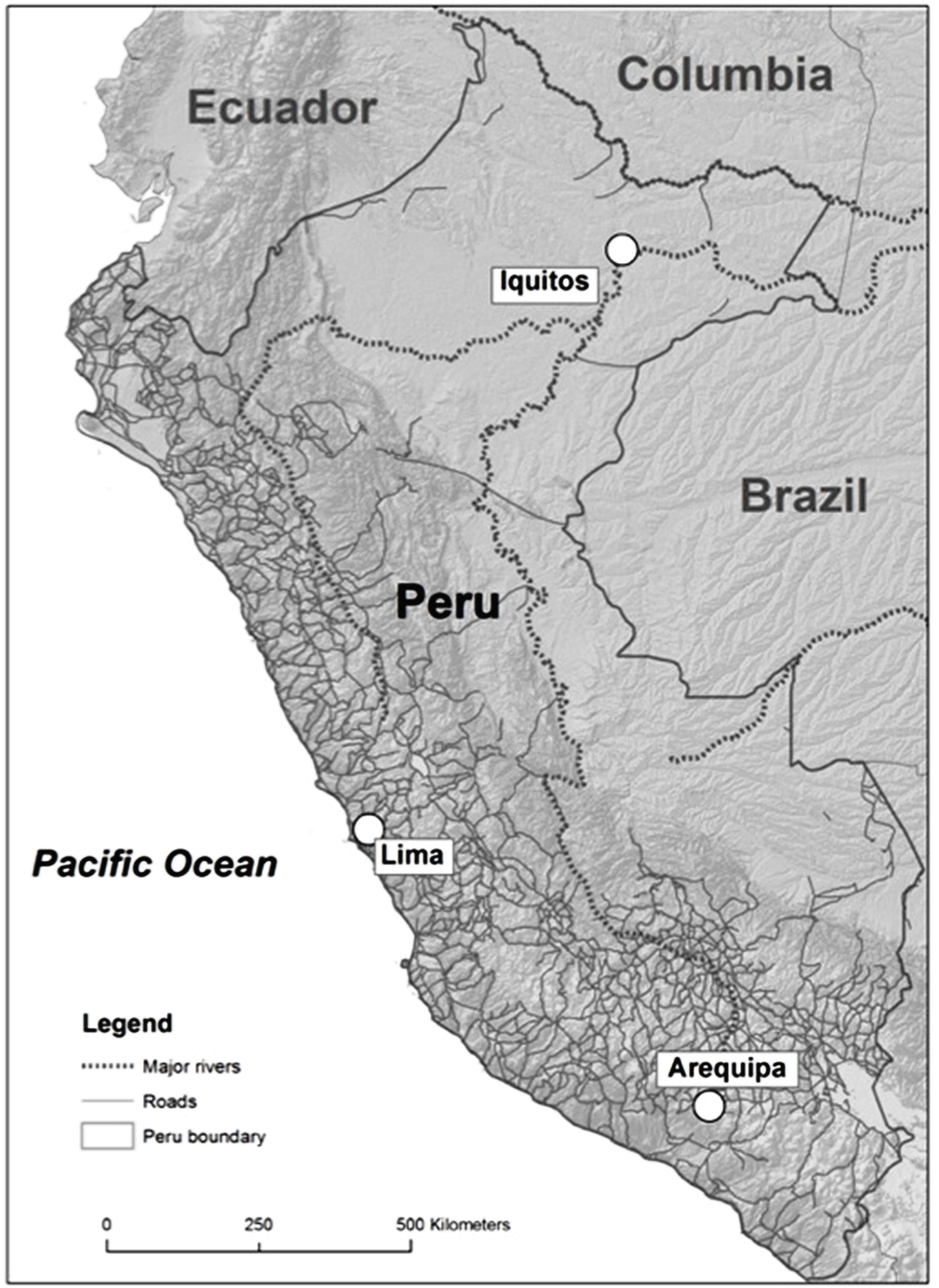
Three sites in Peru were selected for analysis in this study: Iquitos, Arequipa and Lima. Figure 1 shows the three sites and their locations with respect to Peru. The first study area, Iquitos, is located in the interior of Peru in the Amazon Basin. Iquitos has a population of 437,630 and is the sixth largest city in Peru (World Population Review, 2018). It is the largest city in the world that is not accessible by road, only by air or boat (Ruiz-Calderon et al., 2016). The city grew rapidly in the 19^th century based upon the rubber industry (de Jong, 2012), the economy has since diversified to include timber, some minerals, agricultural products, and significant tourism (EY, 2015). The average annual minimum temperature is 21ºC with the coolest month being July. The average annual maximum temperature is 31ºC with the warmest month being September (Weather and Climate, 2019).

Figure 1. Location map of three study sites in Peru: Arequipa, Iquitos, and Lima.

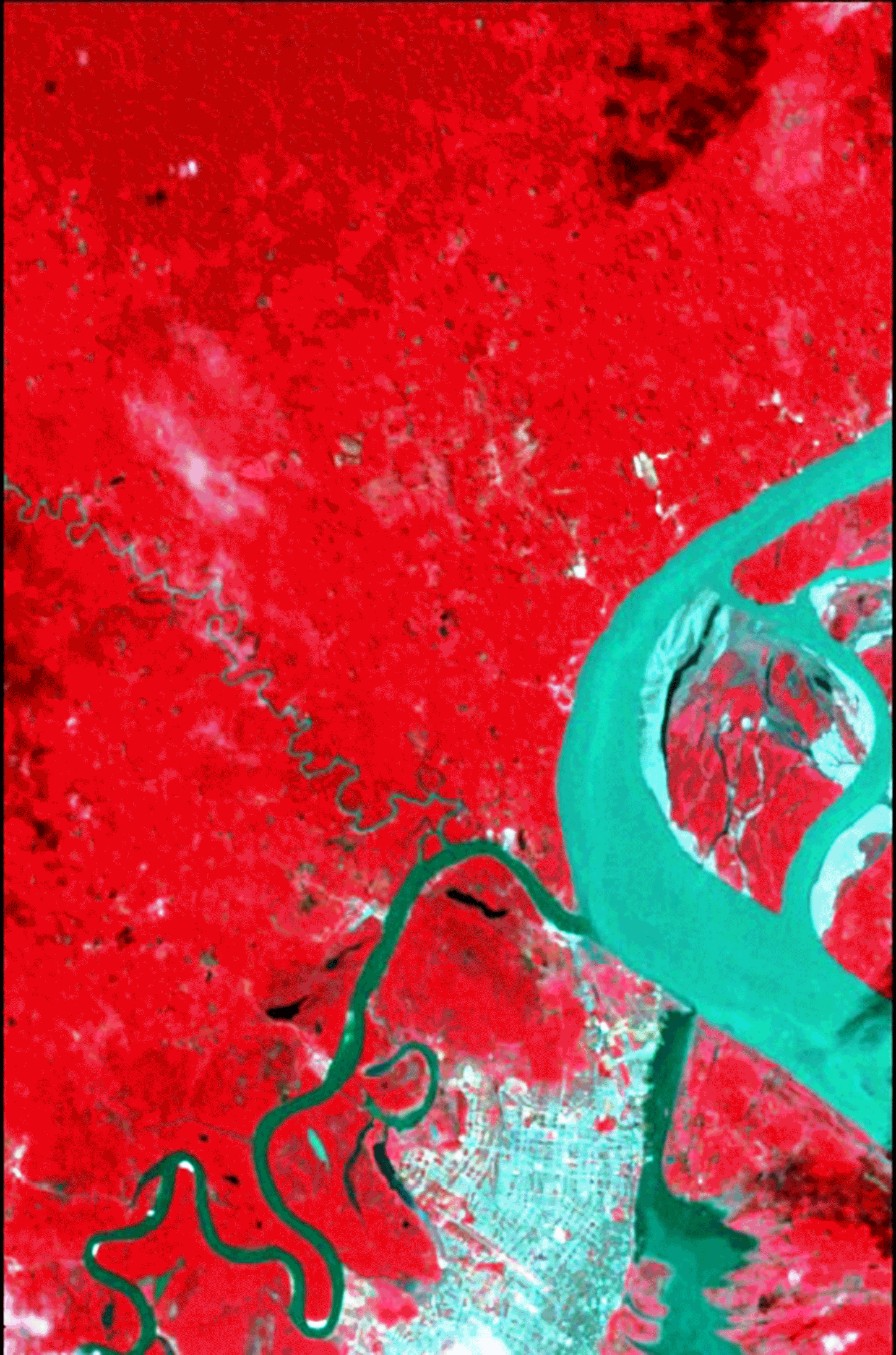
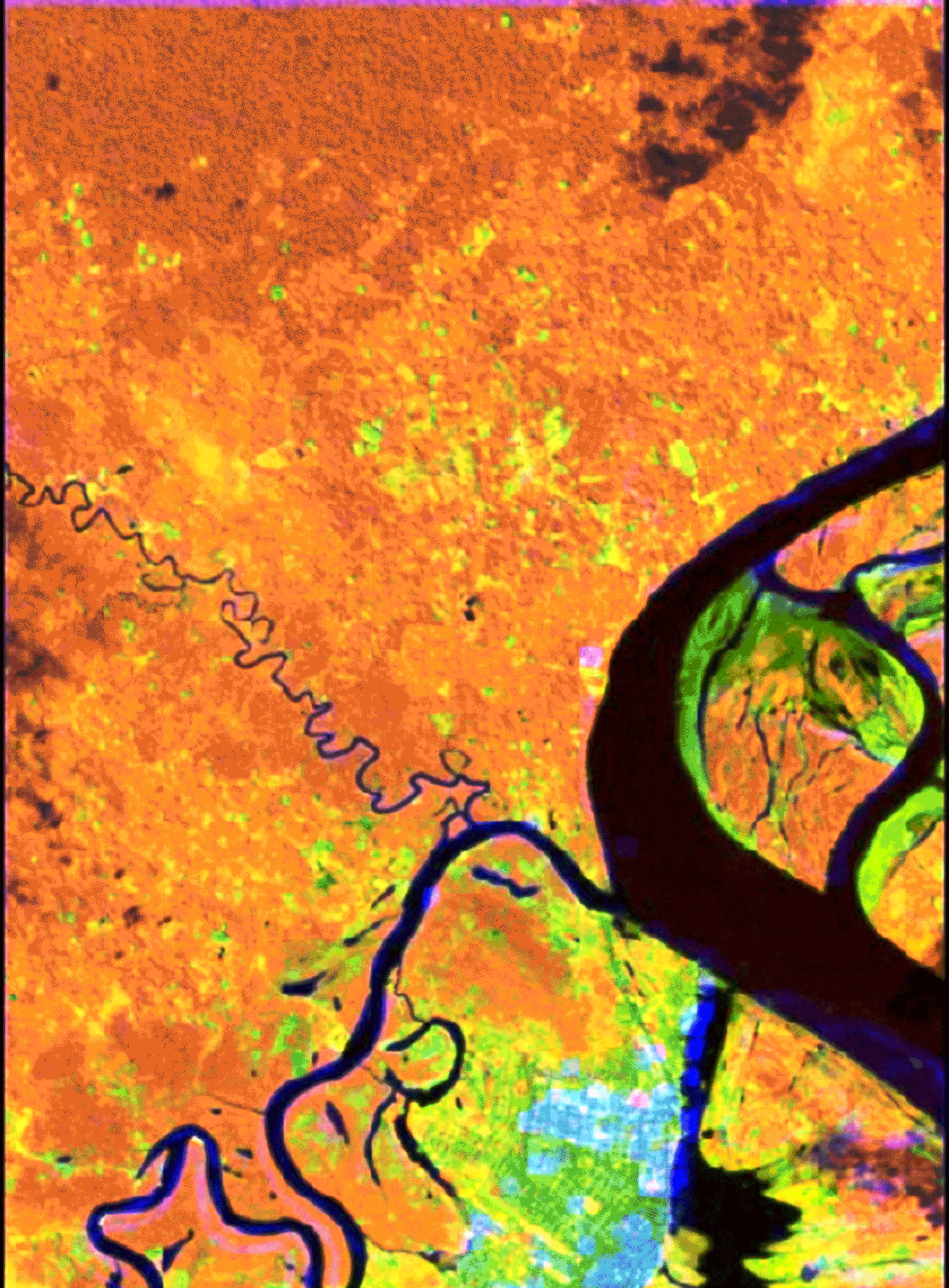
Figure 2 is a false color composite (bands 2, 3 and 4 in B, G and R) Landsat Thematic Mapper (TM) image for Iquitos. The image was captured on 27 July 2007 and has an approximate scene width of 14 km. The primary features in the Iquitos image are the silt laden Amazon river and tributaries to the west and the city of Iquitos to the south. The other features of the image include smooth textured and vibrant red closed canopy forest to the north. Mixed agriculture and secondary forest, in much of scene, is visible with coarser texture, and more mottled red and pink tones.

Figure 2. Landsat TM subset for Iquitos.

Arequipa, the second study area, is the second largest city in Peru. The current population of this city is 841,130 people (World Population Review, 2019). It’s located in the southern part of Peru and is about 100 km from the Pacific Ocean. Arequipa is a West Coast Desert with a very hot and dry climate. The average annual minimum temperature is 6ºC with July being the coolest month. The average annual maximum temperature is 22ºC with the warmest month being March (Weather and Climate, 2019). Arequipa is a very industrial city with most irrigated agriculture occurring on the periphery.

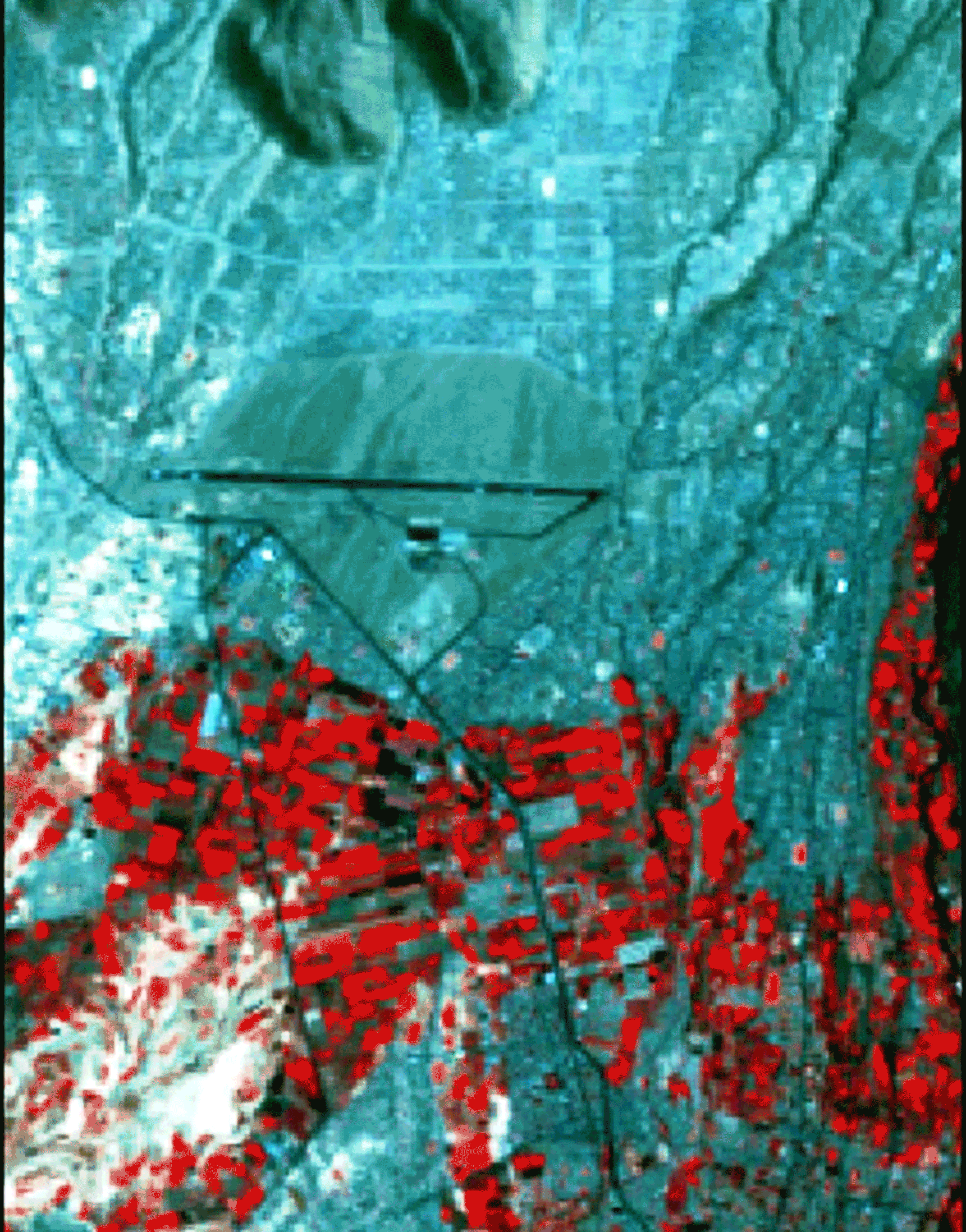
Figure 3 is a false color composite (bands 2, 3 and 4 in B, G and R) Landsat TM image for the Arequipa study area. The image was captured on 12 October 2009 and has an approximate scene width of 6.5 km. The sub-scene is dominated to the north by the extensive urban features of the city in blue grey tones with considerable texture. The airport is located in the central part of this northern area. Some small rectangular parks, visible in red tones, are also located within the built-up areas. This is a common planning feature in this region and typically occurs in the center of residential blocks. Larger commercial and industrial buildings are noticeable by visibly coarser texture, especially to the southwest of the airport. To the north of airport there is a large area of bare soil in similar blue grey tones as urban but with a smooth texture. The most prominent landform features in the study area are the Andes Mountains to the north of the city. To the south, there is a large and highly reflective salt flat. This southern region also contains many irrigated agricultural fields in red tones.

Figure 3. Landsat TM subset for Arequipa.

The third study area, Lima, is the capital of Peru with a very long history that predates European entry into the Americas. Lima is the largest city in Peru with a population of 9,751,717 people (World Population Review, 2019). The city is the largest financial and industrial Centre in Peru with an estimated 7,000 factories producing textiles, clothing, and multiple food products (Hoge, 2014). Located on the coastal plain of the Pacific Ocean, Lima has a mild climate and is very dry as it is also a West Coast Desert (World Fact Book, 2019). The average annual minimum temperature is 17ºC with the coolest month being August. The average annual maximum temperature is 22ºC with the warmest month being March (Weather and Climate, 2019).

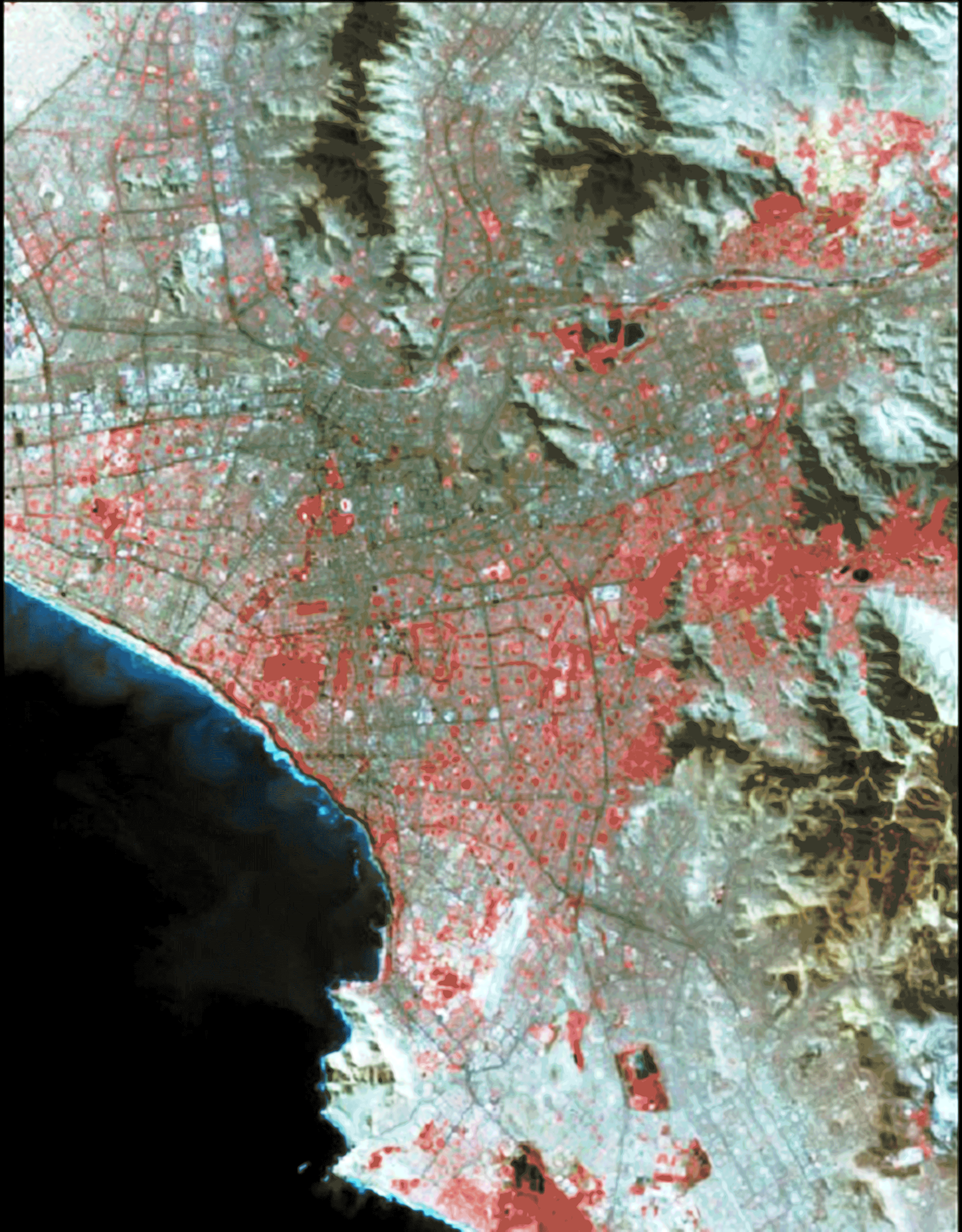
Figure 4 is a false color composite (bands 2, 3 and 4 in B, G and R) Landsat TM image for Lima. The image was taken on 5 May 2015 and has an approximate scene width of 23 km. The Pacific Ocean is in the southwest of this image. Much of the scene contains built up areas of residential, commercial, and industrial uses indicated by blue grey tones. The presence of vegetation is visible by red tones within the urban landscape. The northeast part of the sub-scene contains considerable mountainous terrain.

Figure 4. Landsat TM subset for Lima.

3 . DATA

This study uses both optical and radar imagery. The optical imagery was collected from the Landsat 5 TM sensor from the United States Geological Survey Earth Explorer online platform (USGS, 2019). All seven spectral bands of this imagery were used in this study. The spatial resolution was 30 m for all bands except the thermal band which was 120 m. Radar imagery was collected from the PALSAR sensor on board the Advanced Land Observation Satellite spaceborne platform. This sensor uses L-band radar with the collected imagery having a spatial resolution of 12.5 m. Two polarizations of the PALSAR sensor, Horizontal-Horizontal (HH) like polarization and Horizontal-Vertical (HV) cross polarization bands were acquired for the three sites from the Alaska Space Facility.

Remote sensing data are a compilation of two components: the spectral brightness value for each pixel in an image scene and the spatial arrangement of these pixels. While spectral brightness on its own is valuable for separating features that are very contrasting (e.g. dark features such as wet soils versus bright features such as clouds), for many complex environments (e.g. urban areas and human settlements), spectral brightness on its own is insufficient for separating between features in an image scene. Such features, however, are often more easily distinguished by their spatial characteristics compared to their spectral characteristics alone (Nyoungui et al., 2002; Mahabir et al., 2018). This spatial information can be extracted using various textural measures, the most commonly used being derived from the gray-level co-occurrence matrix (GLCM) (Haralick et al., 1973).

While texture can be extracted from any type of imagery, in optical imagery, the chemical, physical, and biological characteristics of features within the image are provided. This is in comparison to radar imagery, which are associated with the shape, structure, and dielectric properties of features (Pereira et al., 2013). This makes radar data more suitable for deriving texture since it better captures form and structure type properties of features, which can be used to help better distinguish between LULC features. In some cases, image texture extracted from radar data have yielded better classification results compared to the original radar images themselves (e.g. Kiema, 2002; Lloyd et al., 2004; Pathak and Dikshit, 2010). Further, additional research has shown that combining the original radar and derived texture can lead to improved classification accuracy for different LULC features (Herold et al., 2003; Dekker, 2003; Herold et al., 2004). As such, given that the aim of this study is to maximize separation between LULC features in remote sensing imagery, texture formed a major component of this study. Specifically, variance texture layers were extracted from the GLCM from each of the collected radar bands. Variance texture is expressed as (Haralick et al., 1973):

\(Variance = \sum_i \sum_j (i-\mu)^2 P(i,j)\)           (1)

where, \(P(i, j)\) is the \((i, j)\)  entry of normalized GLCM \(P(i, j)\) / R,  R is the total sum of P, and  \(\mu\) the mean of the moving window. Texture in this study was computed with an angle of 0^o and distance of 1, and for three different window sizes of 5 x 5, 11 x 11, and 17 x 17. The variance texture measure and window sizes used in this research were specifically chosen based upon their success in recent LULC classification studies (Idol et al., 2015a, 2015b).

Table 1 contains the list of bands in the data stacks and the image dates for the three study locations. The TM thermal band was deleted from the Lima data stack because as stated later on in this study, it did not prove useful in the other two sites, thus limiting comparison across sites. As will be discussed in the results, this deletion does not change the overall conclusions for this study site. In addition, for Lima, the largest texture window size did not function in the separability analysis, most likely because of the complex urban surface landscape and the difficulty of obtaining viable texture values over larger windows. Consequently, the variance HH and HV texture layers at the 17 x 17 window size for Lima were also excluded from further analysis.

As with other studies that examine data from different sensors, acquiring imagery for the same time for different sites can be challenging. This can be specifically seen with the three sites as in Table 1. With respect to the three study locations, this was primarily due to cloud cover and fog conditions in the optical imagery used in this research. For Iquitos, the two image dates are within two months and occur within the same year, which should not be an issue. For Arequipa, the same season but one year later for the LULC classes selected should not influence the analysis. The image dates for Lima are more problematic, both because of the differences in years and seasons. However, a close visual examination of the various LULC classes in the data used for Lima showed that the classes did not change significantly over that time frame. Thus the temporal gap in image dates is not expected to influence the analysis of this study.

Following the collection of imagery and the derivation of the various texture layers, the nearest neighbor algorithm was used to resample all TM data to 12.5 m (the spatial resolution of the finer radar data). The original TM data were in 8 bit radiometric resolution while the PALSAR was in 16 bit.

As will be discussed in the next section, the PALSAR data were rescaled to 8 bit radiometric resolution and all data were co-registered and layer stacked.

In order to understand the link between the statistical properties of the data stack and features in the image bands as they relate to each site, Table 2 contains the band statistics for the Iquitos site as an example. The high mean for band 4, near infrared, is understandable since much of the scene is heavily vegetated. Similarly, the higher mean for band 5, mid-infrared 1, is also responsive to the extensive vegetation. Given the tropical location, the high mean for band 6, thermal infrared, is expected. The means and standard deviations for the original PALSAR (bands 8 and 9) are the lowest, however, the derived texture bands among the highest. The variance texture bands, 10-15, which are increasing in window size, generally indicate a reduction in mean values and standard deviations with larger windows. This is understandable as the larger window sizes are basically a filtering or smoothing of the data.

Table 3 lists the LULC classes for each of the three sites. For each class one area of interest (AOI) was selected for spectral signature extraction. The number of and specific classes were limited by the landscapes of each study site and thus vary from site to site. The specific classes used in this study were selected based on various factors, including, their ability to adequately reflect the LULC at the three study sites, their extractability from the coarse image data sources used, and their persistence across images dates for each site.

Iquitos had a fewest number of identified classes. The city of Iquitos provided an urban site but it was not possible to separate this area into subclasses of residential and industrial based on the imagery used. Both classes were therefore grouped into an urban class. As shown in Figure 2, there are areas of relatively unchanged tropical rainforest to the north of Iquitos study area indicated by vibrant red with a smooth texture. The highly turbid Amazon River provided a water site and surrounding the city are areas of mixed agriculture and forest with more texture. These areas have secondary growth forest, pastures, and various crops.

In Arequipa, the residential location was characterized by smaller structures and a very organized pattern of blocks of residences surrounding open areas. These appear as a red square in the color infrared TM image composite. The commercial and industrial AOI had larger buildings. Two agricultural fields which appeared to have different crops were also identified. There is a large bare soil area (light blue in the image scene) to the north of the airport and a highly reflective salt flat area in the south of the image scene in Figure 3. Unlike the other two locations, there are no water features.

The Lima subscene, like Arequipa, has extensive areas of residential and commercial/industrial evident by the relative size and organization of buildings. The clear, deep Pacific provided an ocean AOI as did one of the larger urban parks indicated as a red tone. There are regions of bare soil, typically blue toned, and on slopes to the north of the city some dark areas that are also relatively bare but with brown tones, most likely related to the soil and geologic materials. It should be noted that while the classes used in this study are generalized and limited in number, for a selection and relative comparison of image bands, they were considered sufficient. At a future research stage based upon results from this study, more detailed classes might be incorporated such as multiple crops types.

4 . METHODOLOGY

In the first part of this study spectral signatures were extracted for each of the LULC classes using AOI polygons. To reduce spectral confusion between LULC classes, each class was carefully selected using visual analysis and as large an AOI as possible was identified. As an example, for the Lima study area, very large polygons were selected for ocean (124,271 pixels), and industrial and commercial (108,915 pixels) classes. The other classes had smaller AOIs and total number of pixels: residential (68,801), urban (2,985), bare soil (5,766), and dark soil (18,301) pixels. This is a result of the much smaller number of pixels comprising these features, both in terms of the entire study area and with respect to their spatial distributions.

The second part of this study evaluated the use of separability measures to determine the single best band, and band combinations for different numbers of bands. There are various measures of separability for evaluating spectral signatures in remote sensing. The three measures initially evaluated in this study were divergence, transformed divergence, and Jeffries-Matusita. The results for transformed divergence and Jeffries-Matusita for different band combination (e.g. best single, two, and three bands), however, became saturated at their maximum value for many class pairs. This resulted in many band combinations having average and minimum values equal to the maximum values of 2,000 and 1,414 for transformed divergence and Jeffries-Matusita measures, respectively. Therefore, only the divergence measure was used to evaluate bands.

Divergence, a measure of statistical distance between two classes, provides information on their spectral separability. Unlike the transformed divergence and Jeffries-Matusita measures, however, the divergence measure has no upper bound, that is, it does not saturate (Chandra and Ghosh, 2006). It’s an indirect estimate of the likelihood of correct classifications between groups of different band combinations (Swain et al., 1981). Discussions of separability measures, including some of their disadvantages, can be found in Richards (2013). The formula for divergence is given as (Swain et al., 1981):

\(D_{ij} = {1\over2}tr[(Cov_i-Cov_j) (Cov_i^{-1}- Cov_j^{-1})] {1\over2}+tr[(Cov_i^{-1}- Cov_j^{-1}) (\mu_i-\mu_j) (\mu_i-\mu_j)^T]\)  (2)

 where,   i and j are the two classes or spectral signatures being compared, Cov and \(\mu\) are the covariance matrix and mean vectors for classes i and j, tr[] is the trace of a matrix, and T is the transposition function.

In this study, the average divergence values were used to determine the optimum class separability between LULC classes and the best bands to be used prior to image classification. The average divergence value is expressed as (Richards, 2013):

 \(div_{avg} = \sum_{i=1}^m \sum_{j=1}^m p(w_i) p(w_j) Div_{i,j}\)       (3)

where,  m is the number of classes, \(p(w_i)\) and \(p(w_j)\) are the prior class probabilities for classes i and j, and \(Div_{i,j}\)  is the divergence value between classes i and j, respectfully.

A concern in this study was the combination of different radiometric resolutions between the TM (8 bit) and PALSAR (16 bit) data. The specific question addressed; should all the data be rescaled to the same radiometric resolution, and what impact this decision would have on the selection of the best band combinations. To answer this question, separability measures by band and using the same AOIs were obtained for the combined 8 and 16 bit data stack. A second experiment rescaled all data to 8 bit. The results of these experiments were identical in separability values by band and selection of best band combinations. Thus, the radiometric resolution of all data was consistently set to 8 bits for analysis.

5 . RESULTS

5.1 Land Use/Cover Class Statistics

The spectral signatures (digital number and standard deviation) were extracted for the various LULC classes for all three sites and examined. Understanding the relationships between these signatures is important in understanding the LULC class pairs and average divergence values. As an example, Table 4 contains the spectral signatures for Iquitos. Water, as would be expected, has low standard deviation but the mean values in the shorter wavelengths are quite high, even higher than the forest and mixed forest/agriculture classes (as indicated by the values in band 6). This is in part a function of the tremendous sediment load of the water as can be seen in Figure 2, and perhaps because of the mid-morning acquisition time of the imagery as well. Also, as expected, the backscatter for the PALSAR radar and derived texture measures has very low means and standard deviations for water as it is a specular feature.

The forest and mixed forest/agriculture classes have very similar statistics in all bands and the signatures are generally typical of green vegetation. The mean values for the near infrared band is very high compared to values in the visible bands for all classes. In both bands 4 and 5, the mixed forest/agriculture have higher means than the closed canopy forest, which is a result of the agriculture having higher near infrared reflectance than the forest. The very low radar backscatter values (bands 8 and 9) are possible due to cleared agricultural fields. These two classes also have lower values in the thermal infrared compared to the water or urban LULC classes. As would be anticipated, the texture means and standard deviations decrease with increasing window size.

The urban signature has similar means in the first four TM bands, which helps explains why in Figure 2, it appears relatively light grey or blue grey in this false color image. The standard deviations for these four bands are considerably higher than the other LULCs, which is a function of surface variations in the urban landscape. The urban area is also the warmest LULC in the sub-scene. This class has almost identical mean backscatters for the two PALSAR bands as the forest and mixed forest/agriculture but higher standard deviations typical of the varied components of urban features. As expected, the urban radar texture measures have much higher means and standard deviations than any other class. It is uncertain as to why the mean texture bands do not follow a pattern of lowering of values with increasing window size, especially for the urban signature.

5.2  Best Single Band and Band Combinations

Based on the spectral signatures for each site, the divergence measure was used to determine the best bands that would result in the highest classification accuracies. This was done for the best single band, and then the best two, three, four, five, and six bands etc. until all bands were considered. The selection of individual and band combination was based upon the average divergence value for all class pairs and for each spectral signature. The divergence values for individual class pairs were also examined to better understand how these values relate to surface features and their spectral signatures. The subsections that follow present the results of this analysis.

5.2.1 Best Single Band

Table 5 contains the ranking by average class pair divergence values for the three Peruvian study sites. Although each of the study sites was unique with respect to their composition of LULC classes, there were similar results with respect to the top eight bands’ rankings. The best band in all three locations was one of the TM optical bands. For Iquitos, the best band was the TM near infrared band. For Arequipa, the best band was the TM red band. Finally, for Lima, the best band was the first TM mid infrared band. Further comparing the utility of these TM bands, the results in Table 5 show that, with the inclusion of the second TM mid-infrared band, these visible and near infrared TM bands were among the top eight bands for all study sites. Conversely, the TM visible blue and green bands rank low among the TM bands and the thermal band is consistently the least useful of all the TM bands in both the Iquitos and Arequipa sites. Given the coarser spatial resolution of the thermal data (i.e. 120 m compared to 30 m for all other TM bands) and the expected limited variation in 

surface temperatures in the Lima study site when these data were obtained, the exclusion of the thermal band for Lima would not be expected to provide results different from the other sites. As previously stated, unfortunately the largest texture window (17 x 17) was not included for Lima.

With respect to the derived texture bands, the variance texture for the largest windows was among the highest ranked bands. For Iquitos and Arequipa, the second highest ranking band was the HH texture at 17 x 17 window size. For Lima, the coarser texture window HV variance 11 x 11 texture band is ranked fourth after three TM optical bands. Conversely, compared to the coarser texture data, the two original PALSAR polarizations were among the lowest ranked bands.

5.2.2  Best Two Bands

The best two bands for Iquitos were the TM near infrared and the PALSAR HH variance texture at a window size of 17 x 17; these were also the two best single bands as shown in Table 5. These results seem reasonable as these bands are from two very different types of remote sensing data, representing different wavelengths and physical properties of the landscape (represented by derived texture values).

Similar to Iquitos, the best two bands for Arequipa were also from two different wavelengths, one of which was also a texture band. The best two bands for Arequipa were the TM visible red and the PALSAR HH variance texture at the largest (17 x 17) window size. For these two bands, the highest class separability was between bare soil and agriculture. The lowest class separability was between bare soil and residential, as well as between the two agricultural classes as both pairs had the same low divergence value. These high and low separabilities are reasonable based upon their AOI signature class statistics. For the bare soil and agriculture 2 classes, their respective mean signatures and standard deviations were 88/3.5 and 53/4.3 in TM visible red, and 8/8.0 and 188/59.3 in the HH variance texture 17x17 bands, respectively. The low standard deviations for the visible red together with the difference in means create considerable separability. Likewise, while the mean and standard deviation for the agriculture 2 texture is high, these values are very different than those for the bare soil LULC class and thus quite separable. For Lima, the best two bands were the TM mid infrared 1 and the PALSAR HH variance texture at 11 x 11.

5.2.3 Best Three Bands

The best three bands for Iquitos were the TM near infrared, TM mid infrared 1, and the PALSAR HH variance at a 17 x 17 window. Similarly, compared to the results for the best two bands for all sites, these best three individual bands represent very different types of remote sensing data. With respect to the highest average divergence values for all class pairs, there are considerable differences for specific class pairs. The water and urban LULC classes had the highest class pair divergence value followed by water and mixed forest/agriculture, and then water and forest. These results are understandable following the examination of the image sub-scene and the class statistics in Table 4. The lowest class pair divergence was between forest and mixed forest/agriculture. The best three bands for Arequipa were the TM visible red and near infrared bands, with the PALSAR HH texture window of 17 x 17, while for Lima the best three were the two TM mid infrared bands and the largest HV texture window.

Selection of the best three bands is very important in remote sensing for creating color composites, which are used for viewing imagery and for the manual extraction thematic information. The best three band combination for Iquitos was examined visually in different color and band assignments, with the best image shown in Figure 5. This image is a false color composite consisting of PALSAR variance texture at 17x17 window, TM mid infrared 1, and TM near infrared in B, G, and Red. The approximate scene width is 14 km.

Figure 5. Best three band combination for Iquitos.

This figure is not significantly different than the standard color infrared composite in Figure 2. The forest to the north is more distinct in Figure 5 as is the mixed forest/agriculture, however, the water LULC class remains visibly about the same. Also, the urban area in Figure 5 is less well delineated compared to the color infrared image.

5.3  Other Band Combinations

The best four bands from 1365 possible combinations for Iquitos were TM visible red, near infrared, and mid infrared together with the PALSAR HH texture band at 17 x 17. The best five bands added a second HH texture band but at a 5 x 5 window to the best four bands. The best six added a third texture band, HV at 17 x 17 window, to the best five bands. The results for Arequipa and Lima were similar in the lack of utility for the original PALSAR data, the TM thermal, and the shorter TM optical bands.

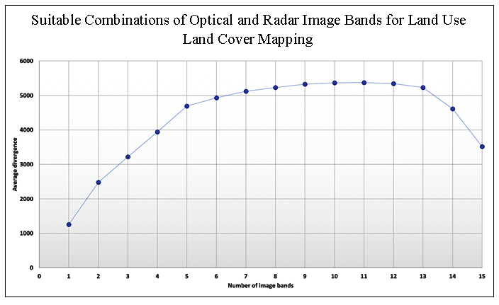
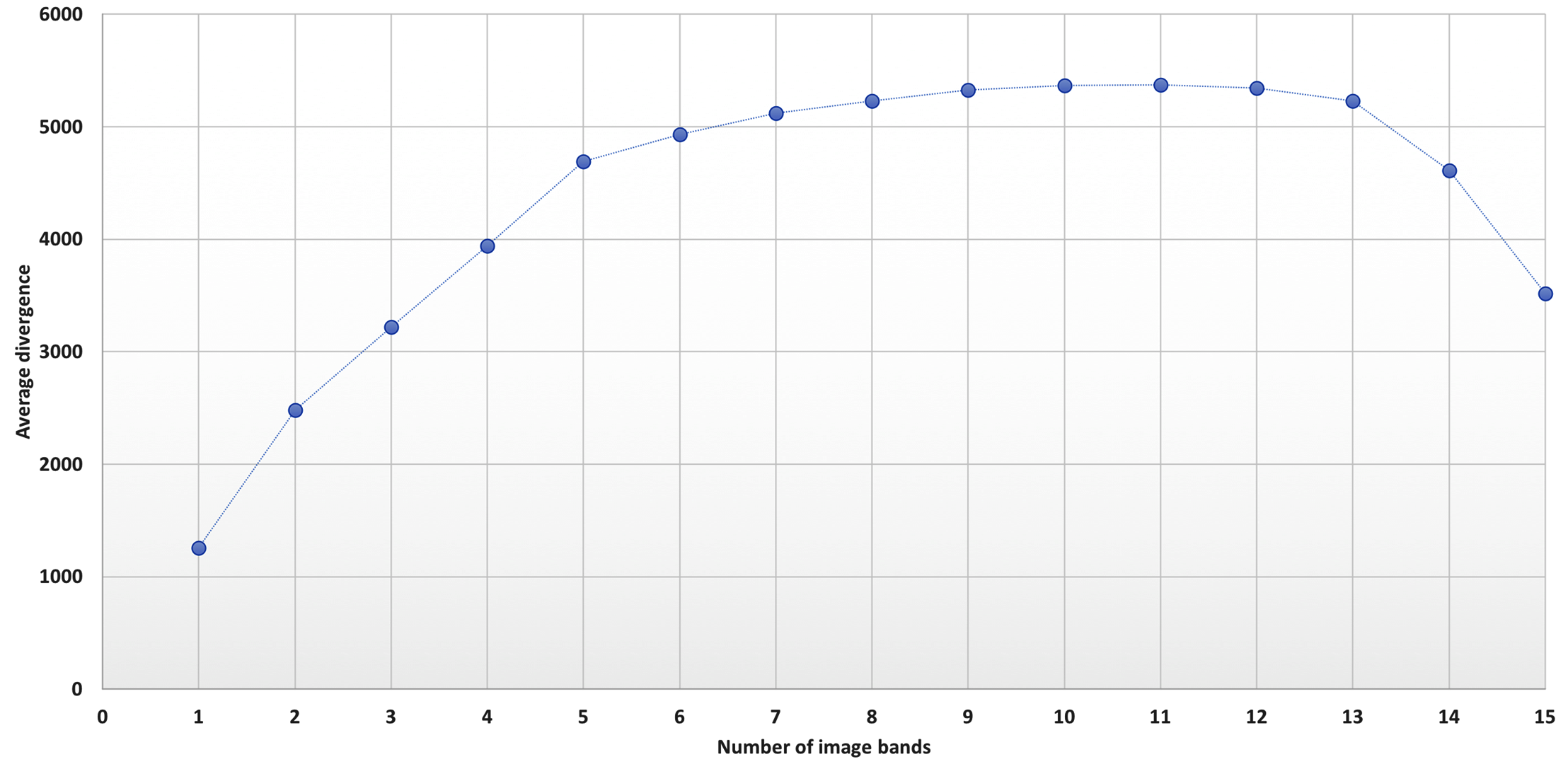
As shown in Figure 6, the divergence values follow an expected pattern of initially increasing with the number of bands. This progression starts with the best individual band for Iquitos at an average divergence value of 1287 and increases steadily to a peak divergence value at 5496 with 11 bands. Following this point the divergence value decreases to a low of 3609 with the inclusion of all 15 bands. However, as illustrated in Figure 6, there is minimal increase in divergence value from 7 to 11 bands with the divergence at seven bands being 5232.

Figure 6. Average class pair divergence values for Iquitos by number of bands.

Similar divergence patterns were observed for the other two study sites. For Arequipa, the optimum divergence value was at 7 bands. For Lima, in which only 12 bands were used, the maximum divergence was at 8 bands, however, with minimal increase in divergence value moving from 5 to 8 bands. These results suggest that there is a negative effect with the addition of too many bands and for these data sets, there is no reason to include more than 6 bands on average. This information provides important evidence for the use of separability analysis. It not only indicates what bands should be used in the mapping of LULC but also the number of necessary bands for a viable LULC classification.

6 . CONCLUSIONS

Today’s remote sensing user is faced with the challenge of sieving through large volumes of data in order to determine which data are relevant for the intended application. One such application is the extraction of LULC information, an important tool for understanding and monitoring the physical processes affecting the Earth. Traditionally, LULC information has been derived from optical imagery, however, there has been growing interest in the use of radar data to help overcome some of its inherent issues. Further, there has been an increase in the number of studies that combine both optical and radar data in the mapping of LULC. Many of these studies show the resulting accuracies to be higher when compared to the sole use of either optical or radar data. This trend, coupled with the upward growth in the deployment and advancement of spaceborne sensors and platforms (e.g. SmallSats and CubeSats), will continue to see the amount of imagery from which LULC information can be derived increase as well. As an example, a recent analysis showing this upward trend for high spatial resolution imagery found that between 1997 (1 satellite) and 2016 (13 satellites), 79 satellites collecting this type of imagery were deployed (Mahabir et al., 2018).

Towards addressing the need for identifying the most relevant data from large remote sensing data stacks, this study has examined one approach. More specifically, spectral divergence analysis was applied to data stacks consisting of optical, radar, and derived radar texture measures to determine the best single band and band combinations for generalized LULC mapping for three locations in Peru. For the single best band, all three sites showed this band to be an optical band from the TM imagery in the visible red (Arequipa), near infrared (Iquitos), and mid infrared (Lima) parts of the electromagnetic spectrum. The other TM bands with shorter wavelengths and the thermal band were consistently ranked among the lower optical bands. In the case of the PALSAR data, the original data were ranked the lowest for all three sites. Conversely, the largest window derived texture bands were among the top four ranked bands. These results suggest that, in situations where resources are limited with respect to the collection of image data, it would be better to prioritize the collection of optical data for the LULC classification.

With respect to the best band combinations, for all three sites, the best band combinations used imagery that was composed of different data types. For example, for Iquitos, the best two bands were the TM near infrared and the PALSAR HH variance texture at 17 x 17 window size. The best three bands added the TM mid infrared 1 band to the best two bands, with the best four bands adding the TM visible red to this combination of bands. These specific band combinations are understandable, and as discussed in the results, relate to the underlying spectral and physical properties of the various LULC classes for the different study sites.

Further comparing the average divergence values for each band in the data stacks, the divergence values initially increased to a maximum peak and decreased thereafter for all sites. In the case of Iquitos and Arequipa, the maximum divergence value was achieved using 11 bands. However, this increase was marginal moving from 7 bands. Likewise, for Lima, while the maximum divergence was achieved using 8 bands, there was only a small increase in divergence moving from 5 bands. These results suggest that, at least with the data used in this study, there is no need to include more than 6 bands for viable thematic mapping. Moreover, the specific bands required to reach an optimal classification were also identified. The method used in this research can therefore be used as a simple approach to determine which image bands should be collected and prioritized prior to LULC classification. Furthermore, such an approach may also provide a simple first step towards deriving a new LULC nomenclature that may better serve the needs of specific geographic regions for which currently available LULC databases may be inappropriate.

As with any study various limitations have also been identified, which at the same time presents opportunities of future work. First, the specific LULC classes examined in this study were generalized, and while they were considered suitable for a relative comparison of image bands and LULC classes in this research, it would be interesting if a more detailed set of LULC classes were used (e.g. multiple crop types). Second, other data from different wavelengths and sources should be investigated as these could lead to different results. This should include data comprising of different seasons and wavelengths. Third, only one measure of separability was used with the need to further compare and contrast the results of other measures across different sites. Finally, other texture measures should be investigated with the additional need to examine the correlation between derived texture measures at a range of difference window sizes.

Tables

Figures

Conflict of Interest

Abbreviations

References