Keywords

baseflow , land-use change , recession curve , Recession Model , Watershed

1 . INTRODUCTION

River baseflow is the result of interrelation and interdependence of a number of environmental factors, namely geological and geomorphological conditions, soil, climate, vegetation, and land-use dynamics (Kienzle, 2006). Baseflow recession modeling is useful for assessing the capacity of water reserves and what percentage of the total runoff comes from groundwater flow. Aquifers are essential water-carrying layers. These permeable geological formations are located above or between impermeable layers and can store and transmit water in sufficient quantities in the field (Thomas et al., 2015).

There has been significantly increasing trend of studies scrutinizing the impact of anthropogenic changes on the hydrological cycle (Barnett et al., 2008). Human interventions on hydrological systems at a local scale, such as land-use changes, irrigation arrangements by dam systems, and water pumping, continuously alter river flows in most watersheds throughout the world (Gerten et al., 2008).  Urbanization amplifies the effects of changes on the hydrological cycle as it converts vegetation-covered areas into a permanent impervious surface, leading to diminished water storage and infiltration capacity (Nathan and McMohan, 1990). In China, groundwater pumping and river flow diversion have significantly modified the water storage capacity of the Chaobai Watershed (Wang and Xia, 2010).

Various physical land attributes jointly shape baseflow characteristics, as conveyed in previous studies about the mushrooming anthropogenic modifications on the hydrological cycle at a local scale. Research on the slope of baseflow recession curves can be applied to various research objectives at the watershed scale, such as flow separation and evapotranspiration estimation (Szilagyi, 1998) and assessment of aquifer parameters (Brutsaert et al., 1998). This research depends on the characterization of the recession curve, namely the optimization of parameters and baseflow recession coefficient.

The recession behavior of flow hydrographs is widely investigated to understand the hydrological processes of watersheds in the future, including evaluating the geomorphological effects (Biswal and Marani, 2010; Biswal and Kumar, 2013, 2014) and the role of river network dynamics on water storage. The behavior of catchments can be characterized by reducing the sensitivity function related to the non-linear storage-discharge relationship. Lo et al. (2010) developed a parametric model of baseflow behavior to estimate water table depths using a land surface watershed model. Carrillo et al. (2011) analyzed hydrograph recession curves using land surface model calibration based on surface water or groundwater behavior. Staudinger et al. (2011) simulated seasonal baseflow, and the temporal variation is illustrated by different recession curves between hydrological models of baseflow. Baseflow recession models approximate water storage capacity on a watershed scale. For this purpose, Vogel and Kroll (1996), Biswal and Marani (2010), and Shaw and Riha (2012) used a single recession event based on variations in recession curves, and Kirchner (2009) assessed watershed behavior using optimization of the recession curve parameters. Rupp and Selker (2006), Wang and Cai (2009), and Thomas et al. (2013) developed a different numerical approach to characterize the storage-discharge relationship.

Baseflow recession curves are generally expressed as natural flow storage capacity, where recession curves contain valuable information about the characteristics of storage and aquifer. Hydrograph recession curves represent the theoretical relationship between aquifer structure and groundwater flowing into the river channel. This theoretical relationship is often described empirically using a baseflow recession curve. Baseflow recession can be understood by estimating its contributing factors, namely physical characteristics of the watershed, using modeling and recession calculation procedures. The recording stages of time-series discharge data create particular difficulties in selecting a recession model. Baseflow recession coefficients are calculated based on the visualization of flow hydrograph. The inflection point on the recession limb of a hydrograph occurs when surface detention is drained. In some cases, after the inflection point, the river continues to flow using water supplies from channel storage, interflow, and baseflow (Eckhard, 2004). Variations in the baseflow recession are specifically attributable to differences in climate during the recession period and are determined by the onset of the recession, while the amount of flow stored in a watershed depends on aquifer types and antecedent climatic conditions (Thomas et al., 2015).

Perzyna (1990) claims that recession modeling required dataset of at least ten years long. This is particularly challenging in sites with incomplete or very short records, although in some instances, several locations hydrologically have similarity in long flow records (Stedinger et al., 1993). At ungauged sites, a simple regression model can be used to analyze the characteristics of baseflow recessions. Regional regression models are developed to statistically estimate baseflows in watersheds with no gauging stations (Tallaksen, 1991). Based on the description above, this study was conducted to analyze the variation in baseflow recession curves as a function of land-use change in the Keduang Watershed, Wonogiri Regency, Jawa Tengah Province.

2 . MATERIALS AND METHODS

2.1 Study area

The Keduang watershed is administratively located in Wonogiri Regency, Jawa Tengah Province, and has a stream gauge station managed by the Watershed Management Research and Technology Station (WMRTS) for Surakarta under the Ministry of Environment and Forestry (Figure 1 and Table 1). This watershed has 10 years daily discharge data, which are feasible for analyzing variations in baseflow recession curves.

Figure 1. Study area: Keduang watershed, Wonogiri, Jawa Tengah Province

2.2  Research procedure

2.2.1      Baseflow recession curve

This research analyzed the baseflow recession models within the RC 4.0 module (build 12) in the HydroOffice  2012 software. The module is commonly used to model single and master recession curves either manually or with the help of genetic algorithms (Gregor and Malik, 2012b). Of all the recession models in it (Table 2), the linear reservoir was selected based on theoretical considerations, empirical judgments, and best visual suitability. Besides, it supports the analysis of at least ten years of time-series daily discharge data.

2.2.2  Land-use change parameters

Landsat satellite imagery (1: 50,000) from 2000 until 2010, acquired from the Forestry Planology Agency Region XI Java-Madura under the Ministry of Environment and Forestry, was analyzed in ArcGIS 10.3. The satellite data were corrected geometrically using Digital Elevation Model (DEM), with 20m pixels and maximum Root Mean Square Error (RMSE) of 0.5 m. The land utilization was categorized into six classes, namely forest, agricultural land, settlement, vacant land, bush/shrub, and water body. The definition of the thematic category using this six-types classification scheme is presented in Table 3.

The recession curve, as a function of land-use change in the research watershed, was visualized using the graphical modeling feature provided by the Matlab® 2015 software. In this process, the baseflow recession segment is a function of seven types of different land-use change. Curves with varying shapes were visualized based on the optimization of the model coefficient and the smallest RMSE.

The Matlab version 2015 has a group of functions that are rung through the GUI, with open-source codes for modification. The familiar graphical user interface makes an intuitive analysis for an extended dataset possible, with which the variation in baseflow recession curve as a function of land-use change was examined. The linear reservoir equation was selected for recession modeling using 10 years data of land-use change (from 2000 until 2010), resulting in varying recession curves with optimized coefficient and the best residual value.

3 . RESULTS AND DISCUSSIONS

3.1      Master recession curves based on the best MSE

The master recession curves (MRC) were visualized in two ways, namely manually and by genetic algorithm, as described below.

3.1.1 Manual visualization of master recession curves

The manually visualized master recession curves (MRC-manual) were modeled with the linear reservoir equation, and the analysis yielded three parameter values: discharge at initial recession (Q₀)= 9.07, α= 0.079, and recession constant= 0.924. The combined parameters were in the range of optimum baseflow recession constant, as evidenced by Nathan and McMohan (1990) (Figure 2).

Figure 2. Manual visualization of master recession curves

The resulting MRC-manual is comparable to Tallaksen (1995) in a way that higher the recession coefficient, more gently sloping the curve, and vice versa.  A gently sloping curve has sizeable baseflow storage that lasts for a relatively long time, whereas a steep curve reflects a fast and massive release from baseflow storage.

3.1.2 Visualization of master recession curves using genetic algorithm

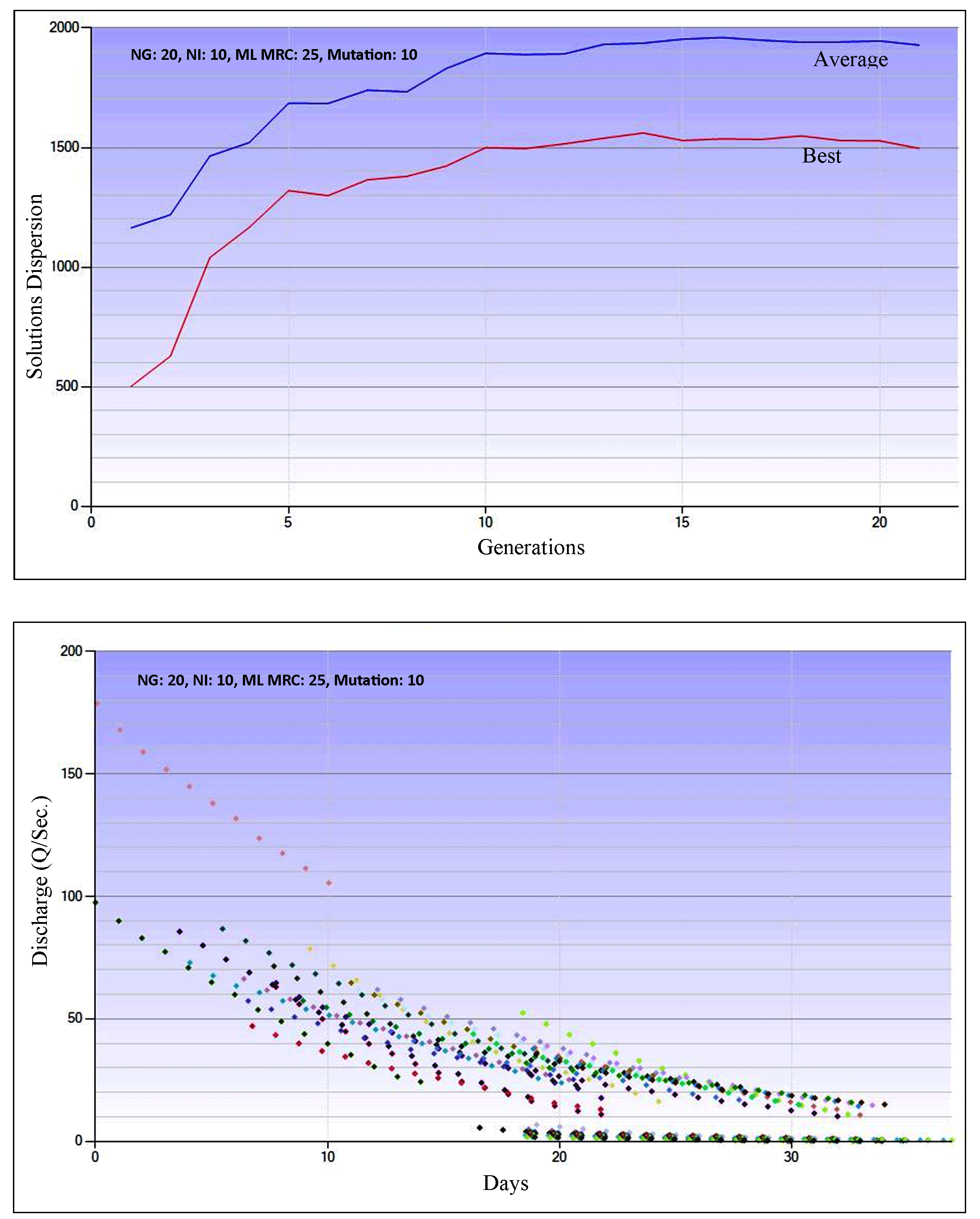
Before the visualization, the parameters used were optimized, i.e., the number of generation (NG) was set at 20, the number of individuals (NI) at 10, the cross of probability at 0.90, the maximum length of the master recession curve (ML MRC) at 25, and maximal dispersion of mutation at 10. The best solution performance for the watershed observed is achieved with t=25 days and a discharge of 100 m³/sec. For optimum and accurate estimates, the algorithm was tested for its performance. Meanwhile, the performance of the evolutionary algorithm is demonstrated through the dispersion of solutions and evolution in the evolutionary cycle. The duration of the algorithm generation depends on the number of selected recession segments, the number of evolution cycles, parallel (individual) solutions, and the maximum length of the master recession curve, as presented in Figure 3.

Figure 3. Visualization of the best solution for optimization of MRC-genetic algorithm

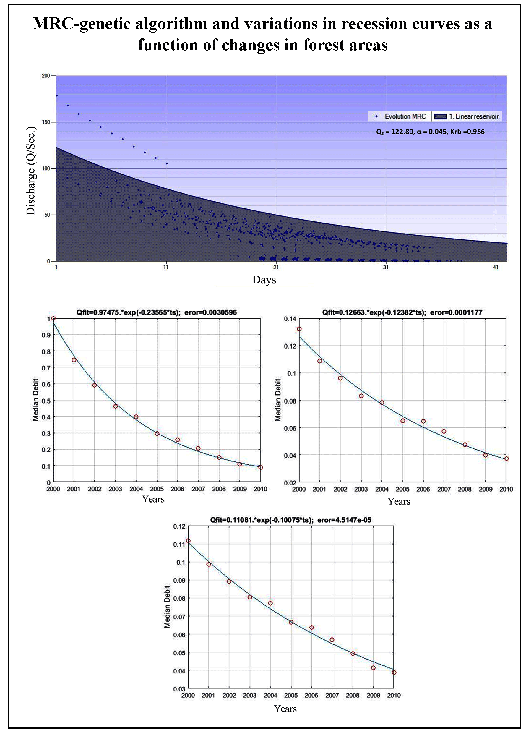
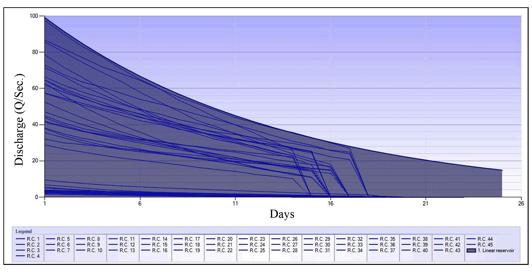
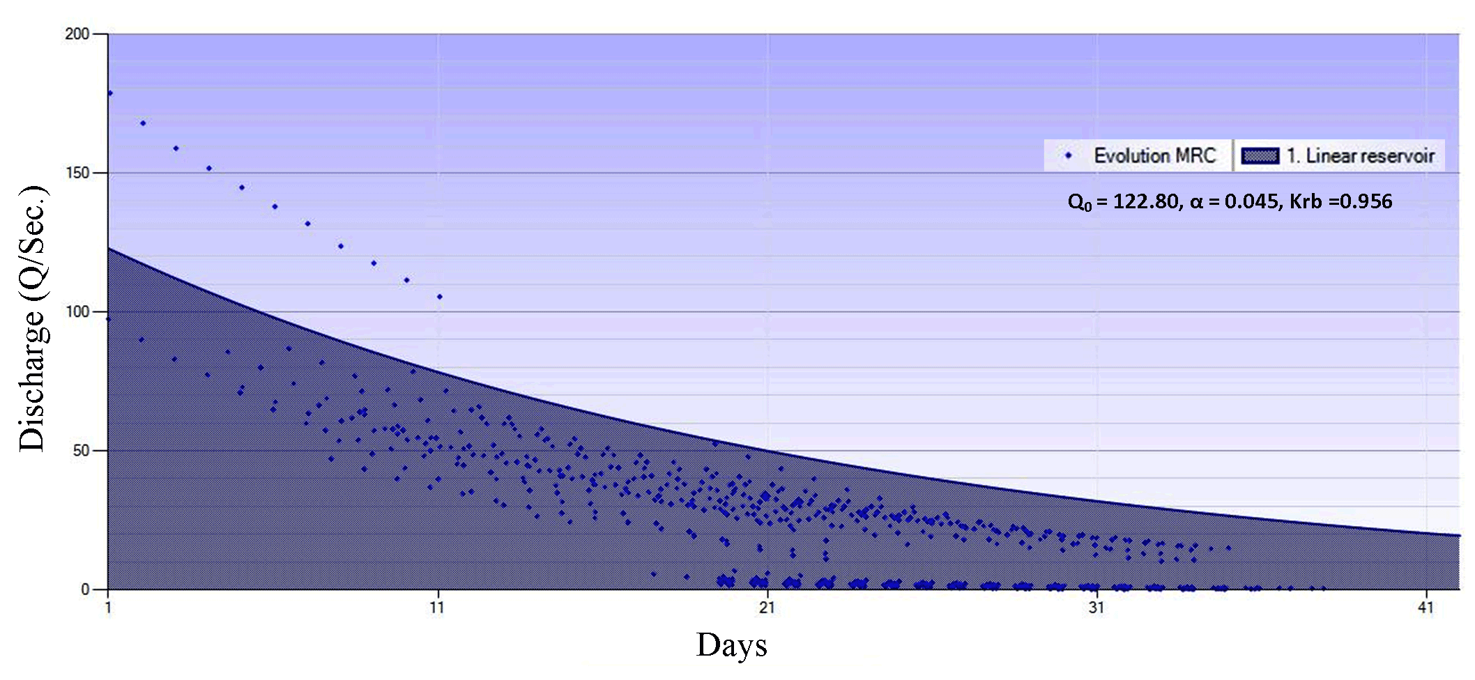
After the best evolution and solution were obtained, the MRC-genetic algorithm was calibrated with the linear reservoir model, and its baseflow recession coefficients and parameters were determined. Optimization of recession coefficient and parameters for Keduang Watershed produced Qo (122.80), α (0.045), and recession constant (0.956). The MRC-genetic algorithm had a gently sloping curve with a recession constant of ± 0.900, meaning that this MRC represents substantially large baseflow storage, as presented in Figure 4.

Figure 4. Visualization of MRC-genetic algorithm

The MRC-genetic algorithm is characterized by baseflow recessions with fairly accurate relevance. Famiglietti et al. (2011) proved that aquifer structures are related to groundwater flowing out to river channels. Kirchner (2009) characterized the behavior of a catchment by reducing the sensitivity function related to the non-linear groundwater discharge-storage relationship. Clark et al. (2011) explain how to deal with the consequences of inaccurate characterization of the processes incorporated in hydrological modeling.

The baseflow behavior was modeled parametrically to estimate water table depths and input these data to the land surface model (Lo et al., 2010). Recession curves were analyzed to illustrate the calibration of land surface models and behaviors of surface water and groundwater (Staudinger et al., 2011). This study visualizes variations in baseflow recession curves as a function of seven types of dominant land-use change into the best curve shape to analyze this causal function.

The RMSE for the Keduang watershed was in the range of 0.04127-2.05645, with a median value of 0.38585. The individual recession segment with the smallest RMSE (<0.1) is considered representative of the characteristics of this segment. The RMSE of the annual recession segment varied from 0.0413 to 0.2030, with a median value of 0.0776.  The calculation results of the recession coefficient and parameters are accompanied by the smallest RMSE calculation.

3.2 Variations in the land-use change in the research watershed

The land surface dynamics of the Keduang watershed were shaped by seven main types of land-use conversion, namely the narrowing of forest area (from 38.68% of the total watershed area to 21.90%), increased conversions of forests to agricultural land (from 5.24% to 9.23%) and settlements (from 4.45% to 9.58%), reduced agricultural areas (from 30.68% to 25.25%), increased conversions of agricultural land to settlements (from 4.41% to 10.35%) and back to forests (from 1.96% to 3.41%), and expanded residential areas (from 13.71% to 18.89%). Meanwhile, the variations in vacant land, bush/shrub, and water body were relatively constant.

From the spatiotemporal perspective, forests are inclined to shrink as more and more of their areas are cleared and used for agricultural and residential purposes instead.  Agricultural and residential areas, as well as the conversion of agricultural land to forests and settlements, continue to increase significantly. These variations were modeled using the Matlab (R) software to analyze their effects on the characteristics of baseflow in the research watershed.

Land uses continuously changed over the ten years (2000-2010) as a result of socio-economic and political dynamics. All processes taking place in the watershed can support human activities. Landforms in a watershed are constantly changing system, and at the same time, ecosystems growing on them are very sensitive to human interventions. More often than not, artificial modifications within and around river channels disrupt the ecological characteristics (Leuven and Poudevigne, 2002). Land-use change can be characterized by the complex interactions between the behaviors and structures of its determinants, including those related to demands, technological capacity, and social relations -all of which control environmental requirements, capacities, and properties (Staudinger et al., 2011).

3.3 Variations in baseflow recession curves based on land-use change

Variations in baseflow recession curves as a function of land-use dynamics represent the different spatial characteristics of the watershed observed. For instance, they may reflect the trends of change in forests, agricultural land, and settlements that contribute to the current conditions of the baseflow recession.  The recession coefficients for variations in land-use change in Kedaung Watershed are summarized in Table 4.

 

Table 4. Curves modeled from variations in land-use and baseflow recession discharge

Classes of land-use change	Recession models	MSEs
Forest to forest (preserved)	Qmodel= 0.9747*Exp(0.2357*ts)	0.0031
Forest to agricultural land	Qmodel= 0.1266*Exp(0.1238*ts)	1.18E-04
Forest to settlement	Qmodel= 0.1108*Exp(0.1008*ts)	4.51E-05
Agricultural land to agricultural land (unchanged)	Qmodel= 0.7628*Exp(0.2015*ts)	2.75E-03
Agricultural land to forest	Qmodel= 0.0465*Exp(0.1141*ts)	1.88E-05
Agricultural land to settlement	Qmodel= 0.1072*Exp(0.0952*ts)	7.78E-05
Settlement to settlement (unchanged)	Qmodel= 0.3359*Exp(0.1542*ts)	7.18E-04

Source: Curve analysis in Matlab® from 2000 until 2010.

 

Based on the recession coefficients, the slope of the modeled curves illustrates the variation in baseflow recession curves, which can be defined as gently or steep sloping. According to the equations listed in Table 4, the types of land-use change represented by gently to steep sloping curves are in the following order: preserved forests (gently sloping), unchanged agricultural land and settlements, the conversion of forests to agricultural land, agricultural land back to forests, forests to settlements, agricultural land to settlements (steep). In conclusion, the conversion of forest to non-forest use, together with the areal dynamics of agricultural land and settlements, alters the capacity of baseflow storage. Forests are known to retain water better and longer than non-forest areas.

3.3.1 Baseflow recession curves as a function of changes in forest areas

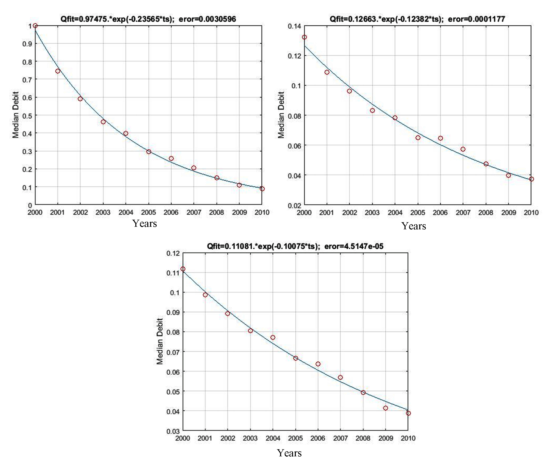
The equations of baseflow recession models as a function of changes in forest areas were as follows: Qmodel= 0.9747*Exp(-0.2357^*ts) for preserved forests (coefficient of the model=  0.2357; MSE= 0.0031), Qmodel= 0.1266*Exp(-0.1238^*ts) for the conversion of forests to agricultural land (0.1238; 1.18e-04), and Qmodel= 0.1108*Exp(-0.1008^*ts) for the conversion of forests to settlements (0.1008; 4.51e-05).  Figure 5 shows that these recession curves were relatively sloping, as evident from 23.57% slower recession in preserved forests, while the curve slopes of forests that had been converted into agricultural land and settlements were 12.38% and 10.08%, respectively. These results indicate that forests, when preserved, have larger storage capacity and can store water longer by 23.57% than the ones converted to non-forest land.

Figure 5. Variations in recession curves as a function of changes in forest areas

 

In other words, this study confirms that forests play a significant part in the hydrological cycle. When the rain starts to fall on dense vegetation, the water is intercepted by the leaves, stems, and branches of emergent and canopy trees. Upon saturation, the retained water is replaced by subsequent rain and drips into the leaves, stems, and branches of the lower canopy structure before it finally reaches the plants on the forest floor, litter layer, and soil surface. The amount of water retained on the surface of the leaves, stems, and branches is called interception or canopy storage capacity, and it largely depends on the shape, density, and texture of the vegetation.

The nature of vegetation canopy is an important element in the interception process. Interception occurs when rainwater falling on the surface of vegetation is retained for a while, and then evaporated back into the atmosphere (water loss) or absorbed by the vegetation. This process lasts during and after rainfall until the surface of the plant dries again.  Every time rain falls on a vegetated area, there is a portion of water that never reaches the ground surface, and as such, does not partake in the formation of soil moisture, runoff, and groundwater. Instead, it either returns to the air or is intercepted by the leaves and litters. Interception plays a crucial role in the hydrological cycle because it significantly reduces the portions of rainwater that reach the ground, specifically in a densely vegetated surface like forests. Therefore, watershed management must take into account this process in its planning and implementation.

3.3.2 Baseflow recession curves as a function of changes in agricultural land

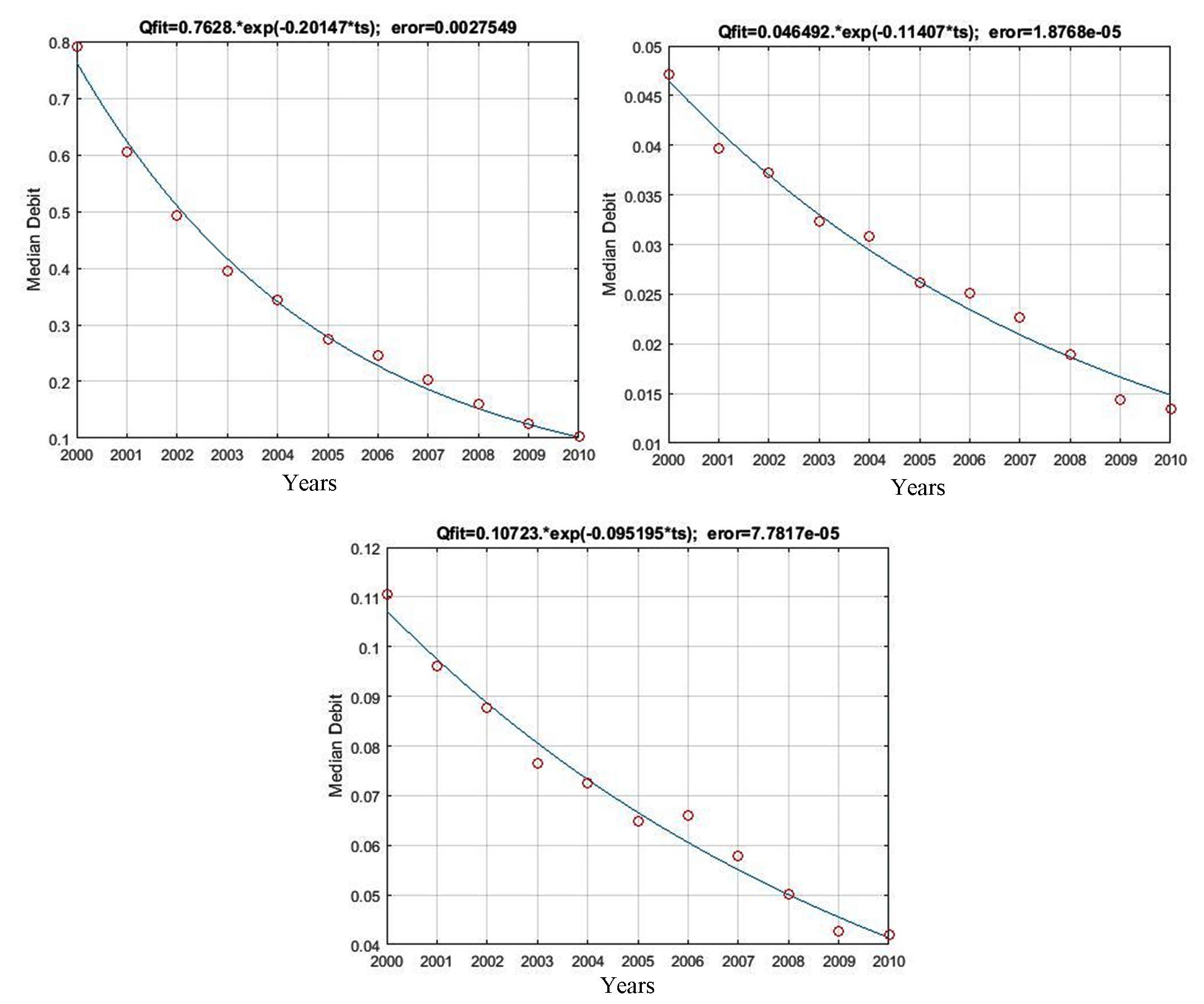
The equations of baseflow recession models as a function of changes in agricultural land were as follows: Qmodel= 0.7628*Exp(-0.2015^*ts) for unchanged agricultural land (coefficient= 0.2015; MSE= 2.75e-03), Qmodel= 0.0465*Exp(-0.1141^*ts) for the conversion of agricultural land back to forests (0.1141; 1.88e-05), and Qmodel= 0.1072*Exp(-0.0952^*ts) for agricultural land to settlements (0.0952; 7.78e-05).  Figure 6 shows that the recession curves as a function of changes in agricultural land were relatively steeper compared to changes in forest areas in general. The curve slope for unchanged agricultural land was 20.15%, followed by 11.41% and 9.52% for the conversion of agricultural land to forests and settlements, respectively. In other words, unchanged agricultural land has a larger storage capacity than the one converted into forests and settlements. Nevertheless, with generally steeper slopes, the entire water storage capacity of agricultural land (unchanged and converted) has a lower yield than that of forests.

 

Figure 6. Variations in recession curves as a function of changes in agricultural land

 

This finding is consistent with the previous studies of forest hydrology, which also detected an extensive conversion of forest to non-forest areas. Significant environmental changes in a watershed can lower the canopy storage capacity, which evidently plays a crucial role in water balance. The greater the canopy storage capacity, the more likely the canopy interception takes place, and higher the amount of rainwater loss that should reach the ground. However, under certain circumstances, the interaction between water that evaporates in vertical interception with the one produced by horizontal interception (i.e., dew interception by forest canopy) is likely to provide additional water yield in some watersheds. Therefore, interception can affect the water balance of a watershed at varying scales due to a local humidity deficit associated with the decreased amount and different sizes of drops of rain falling on the canopy and water escaping to the ground.

Changes in land cover from one type of vegetation to another can affect the annual water balance in a watershed. The shape, density, and texture of vegetation strongly determine interception or canopy storage capacity. Scientific evidence collected since 1960 indicates that interception is much faster than transpiration, and on a watershed scale, the loss of water by interception is a form of real water loss in the water balance system (Ward, 1975). Studies by Hewlett (1961) and Hibbert (1967) in a small watershed in North America found a real increase in water yield as a result of narrowing forest vegetation, while, in other circumstances, there has been a decline in water yield as a result of changes from broadleaf to pine forests. These situations are the consequence of changes in the amount of interception in the watersheds.

3.3.3 Baseflow recession curves as a function of changes in settlement areas

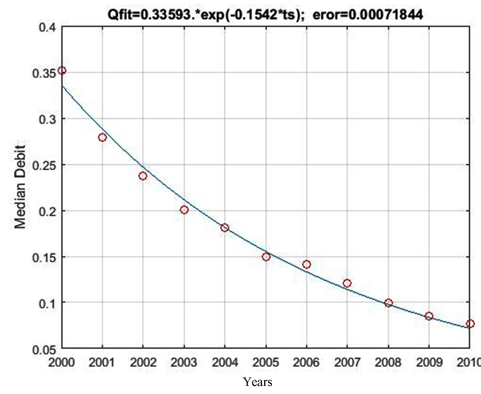
The equation of the baseflow recession model for changes in residential areas was Qmodel= 0.3359*Exp^(-0.1542^*ts) with a model coefficient of 0.1542 and MSE of 7.18e-04. Figure 7 shows that the baseflow recession curve of unchanged settlements was steeper (15.42) than that of preserved forests (23.57) and unchanged agricultural land (20.15). In this case, unchanged settlements have the smallest water storage capacity.

 

Figure 7. Variations in recession curves as a function of changes in settlement areas

 

Overall, the equation indicates that on a watershed scale, forests have the capacity to store water better and longer than the ones that have been converted for agricultural and residential purposes. The baseflow recession curve as a function of changes in forests is more gently sloping than the curves reflecting the dynamics of agricultural land and settlements.

Land use is one environmental attribute that changes very quickly and, as a result, causes various effects on the hydrological conditions of a watershed. If land utilization modifies the landscape of a watershed, then the effect will potentially expand to water yield. To some extent, it can alter the hydrological conditions of the region. More often than not, the conversions of forests to non-forest areas, such as agricultural land and settlements, and of agricultural land to settlements are permanent and extensive (large-scale), leading to changes in water yield and hydrological conditions. Most issues on water resources pertain to the time and distribution of water flow, and for this reason, the integration of many approaches like vegetation management and engineering measures is necessary.

In the hydrological cycle mechanism, rainwater seeping into the soil controls water availability for evapotranspiration. The supply of rainwater into the soil is beneficial for most plants in the infiltration zone and its surroundings. Ecologists and agricultural experts must understand the interrelationship between plants and their water requirements by considering the formation and mechanism of infiltration and surface runoff, especially the plant-soil-water nexus.

Infiltrated water that does not return to the atmosphere by evapotranspiration continues to seep deeper through the soil and reaches groundwater that eventually flows into the river and its surroundings. Increasing the rate and area of ​​infiltration can multiply the amount of flow discharge during the dry season (baseflow) to provide water for various purposes. Depending on soil biophysical conditions, some or all parts of rainwater falling into the ground seep through the soil pores.

The rate of infiltration is dependent on the diameter of soil pores. Under the influence of gravity, rainwater flows vertically into the ground through the soil profile. The capillary force causes water to move upward, downward, and laterally and occurs in soils with relatively small pores. Meanwhile, in soils with large pores, this force can be ignored, and water flows deeper into the ground gravitationally. Infiltration is influenced by, among others, the texture and structure of the soil, initial moisture, biological activities and organic elements, the type and depth of the litter layer, and vegetation or other canopies that cover the soil. Soils with crumb structure have a higher infiltration capacity than clay, and water-saturated soils have a smaller capacity than the dry ones. Dense canopy cover can reduce the amount of rainwater that reaches the ground and, at the same time, the quantity of infiltration water.

Vegetation root systems and litter help increase soil permeability and, consequently, the rate of infiltration. Initial moisture is the most vital element that determines the potential pressure on the soil surface. Decreased infiltration rate makes soil grains expand and fills the soil pores. Vegetation growth requires a certain level of soil moisture, and as such, soil moisture can shape the developing land use. Drought events have more to do with soil moisture rather than the number of rain events in the watershed observed. Soil moisture is beneficial for human life, and when it is too high or too low, it can cause problems for this purpose.

4 . CONCLUSIONS

Variations in baseflow recession curves as a function of seven types of dominant land-use change in Keduang Watershed are represented by these equations: Qmodel= 0.9747*Exp^(-0.2357*ts) for preserved forests, Qmodel= 0.1266*Exp^(-0.1238*ts) for the conversion of forests to agricultural land, Qmodel= 0.1108*Exp^(-0.1008*ts)  for forests to settlements, Qmodel= 0.7628*Exp^(-0.2015*ts) for unchanged agricultural land, Qmodel= 0.0465*Exp^(-0.1141*ts) for the conversion of agricultural land back to forests, Qmodel= 0.1072*Exp^(-0.0952*ts) for agricultural land to settlements, and Qmodel= 0.3359*Exp^(-0.1542*ts) for settlements. These equations represent the slope of the baseflow recession curve, which reflects the water storage capacity of the watershed.

The water storage capacity of preserved forests is 23.57%, followed by 12.38% and 10.08% in forest areas converted into agricultural land and settlements. Unchanged agricultural land has 20.15% water storage capacity, and when converted into forests and settlements, its capacities are 11.41% and 9.52%, respectively. Meanwhile, the unchanged residential areas have a water storage capacity of 15.42%.  Overall, forests can store water better and longer than the ones that have been converted to agricultural fields and settlements.

Tables

Figures

Conflict of Interest

Acknowledgements

Abbreviations

References

5.
Boussinesq, J., 1877. Essai sur la theorie des eaux courantes. Memoires presentes par divers savants a l’Academie des Sciences de l’Institut National de France, Tome XXIII, 1. Imprimerie Nationale, Paris.
18.
Hewlett, J. D., 1961. Watershed management. In report for 1961 South-Eastern Forest Expt. Sta. Asheville, NCUSDA Forest Service, Southeastern Forest Expt. Sta., 62-66.
23.
Kovács, A., 2003. Geometry and hydraulic parameters of karst aquifers- A hydrodynamic modelling approach. PhD. thesis, La Faculté des sciences de lUniversité de Neuchâtel, Suisse, 131.
24.
Kullman, E., 1990. Krasovo-puklinové vody. Karst-fissure waters. GÚDŠ, Bratislava,184.
27.
Maillet, E., 1905. Essai d'hydraulique souterraine et fluviale. Libraire Sci., A. Herman, Paris.
29.
Perzyna, G., 1990. Parameter estimation from short observation series of low flows. In: G. Perzyna (Eds), Derived Frequency Distribution for Low Flows, Dr. Sci. Thesis. Inst. Geophys., University of Oslo, Oslo, 1993, Part 3. University of Oslo, Oslo.
33.
Stedinger, J. R., Vogel, R. M. and Foufoula-Georgiou, E., 1993. Frequency analysis of extreme events. In: D.R. Maidment (Eds), Handbook of Hydrology. McGraw-Hill, New York, 18.55.
35.
Tallaksen, L. M., 1991. Recession rate and variability with special emphasis upon the influence of evapotranspiration. Dr. Scient. Thesis, University of Oslo, Rapp. Hydrology, 25.
39.
Toebes, C. and Strang, D. D., 1964. On recession curves 1: Recession equations. J. Hydrology, New Zealand, 3(2), 2-15.
43.
Ward, R. C., 1975. Principles of Hydrology. McGraw-Hill Book Company, UK.