1 . INTRODUCTION
Unmanned Aerial Systems (UAS) have been widely used in many applications such as vegetation monitoring (Merza and Chapman, 2011); agriculture (Walsh et al., 2018; Marino and Alvino, 2019), hydro-geomorphological assessments (Casado et al., 2016), hydrology, water conservation, water quality analysis (Koparan et al., 2019), river characterization (Casado et al., 2016; Larrinaga and Brotons, 2019), soil management (Oliveira et al., 2019), urban mapping (Noor et al., 2018), disaster management (Yang et al., 2016; Carvajal-Ramírez et al., 2019) including post-fire vegetation analysis (Fernández-Guisuraga et al., 2018). At present, satellite based remote sensing has limitations such as resolutions, availability including frequency and flexibility, complicated image processing, higher costs etc. (Zhang and Kovacs, 2012; Wan et al., 2018) whereas ground-based sensor systems have issues related to mobility (moving one place to another), cost-effectiveness and real time mapping (Zhang and Kovacs, 2012; Sankaran et al., 2015; Caturegli et al., 2019). However, UAS based techniques are useful for survey of relatively smaller area, but for efficient work it needs to be larger than 5 hectors (Wahab et al., 2018). UAS is more efficient tool to bridge the gap between- 1) high expensive satellite and manned areal remote sensing and 2) labors and time-consuming conventional fieldwork techniques of data collection for environmental planning, management and monitoring (Wahab et al., 2018).
The market revenue of UAS based remote sensing and mapping is booming since last decade (Colomina and Molina, 2014; Barbedo, 2019). At the same time scientific community and industry have remarkably involved with publications and production of essential equipment (Colomina and Molina, 2014). Many conferences/meetings were organized in this period and volumes were published by reputed organizations and publishers (Colomina and Molina, 2014). Many commercial, non-profit organizations and governmental agencies are involved and have invested their energies for research, development and applications of the UAS techniques.
Popular terms observed for this technique are Remotely-Piloted Aerial Systems (RPAS), ‘Unmanned Aerial Vehicle’ (UAV), ‘aerial robot’, ‘drone’ (Colomina and Molina, 2014), etc. International Civil Aviation Organization (ICAO) has coined the term RPAS and integrated this technology into ‘international civil aviation system’ (ICAO, 2011). UAS includes: 1) unmanned aircraft (UA), 2) a Ground Control Station (GCS) and 3) a communication data links (Colomina and Molina, 2014). 1) Aircraft trajectory: waypoints, strips, speed, attitude, etc. and 2) mission management: sensor configuration, triggering events, flying directions, etc. are important aspects during the mission. Micro- and mini- UAS vehicles are very sensitive to winds therefore 80% forward and 60-80% cross overlap are suggested to compensate errors occurred due to aircraft instability (Colomina and Molina, 2014). Four types of UAS are parachutes, blimps, rotocopters, and fixed wing systems (Sankaran et al., 2015). Further, stable imaging platforms have been suggested as solution to the problem of wind induced instability in UAV (Yang et al., 2016).
Colomina and Molina (2014) have explained different aspects of UAS: recent unmanned aircraft, navigation, sensing techniques, data processing techniques and photogrammetry. Novelties of the technique are very high resolution (centimeter level), low-cost equipment, powerful, sophisticated computer vision, robotics and geomatic engineering (Colomina and Molina, 2014; Gracia-Romero et al., 2019; Caturegli et al., 2019). Therefore, the advances of the technique are: 1) cost-effective: low weight, slow flight, speed and extended range, (Casado et al., 2016), 2), less fuel (Casado et al., 2016), 3), timely and on-demand data (Casado et al., 2016) and 4) safety mission (Casado et al. 2016). UAS can capture images even in cloudy conditions (Casado et al., 2016). This technique is more useful for large-scale low-altitude imaging and geospatial information (Colomina and Molina, 2014) for policy makers, regulatory bodies and mapping authorities.
UAS applications are detection and quantification of stress plants, prediction of yield, estimations of biomass and canopy cover, classifications of vegetation, assessment of plant heights, etc. (Barbedo, 2019; Oliveira et al., 2019; Durfee et al., 2019). Vegetation indices (VIs) show significant relationship with disparities in ground cover (Schut et al., 2018) including vegetation, soil characteristics (Oliveira et al., 2019), barren and impervious surfaces, water bodies etc. VIs are widely used for analysis of 1) precision agriculture: analysis of crop performance (Buchaillot et al., 2016; Marino and Alvino, 2019; Gracia-Romero et al., 2019), diseased crops/plants (Sandino et al., 2018; Javan et al., 2019), plant nutrients (Walsh et al., 2018), plant phenology (Park et al., 2019), plant height (Fathipoor et al., 2019), 2) preparation of DEM (Themistocleous, 2019), 3) management of covered soils (Oliveira et al., 2019), etc. Durfee et al. (2019) have used VIs for assessing the green cover at watershed level. Carvajal-Ramírez et al. (2019) have calculated fire severity indices for pre- and post-fire situations using MSS imageries captured by UAS.
Walsh et al. (2018) have calculated VIs for Spring wheat thorough growing stages using UAS images and found positive significant relationship between calculated VIs values and measured plant nutrients. Javan et al. (2019) have successfully used UAV based VIs for detection and mapping of diseased Citrus plants. Buchaillot et al. (2016) have analyzed Maize performance in low nitrogen condition using VIs calculated based on UAS-MSS data in Zimbabwe. Marino and Alvino (2019) have analyzed the abilities of high resolution UAU images to detect the spatiotemporal variability of wheat crop in Italy. Caturegli et al. (2019) have analyzed the applicability of NDVI [Normalized Difference Vegetation Index] and DGCI [Dark Green Color Index] for detection of N content in plant life for precision agricultural management using UAS. Eng et al. (2018) and Cermakova et al. (2019) have used the VARI (Visible Atmospherically Resistant Index) for vegetation analysis. Park et al. (2019) have using UAV based color indices to quantify the leaf phenology of trees and species in tropical forest. Marcial-Pablo et al. (2018) have used VIs for estimations of vegetation fractions using UAV-RGB images. Therefore, UAS based VIs are very useful for analysis of plant nutrients, variability in crop performance, vegetation analysis, etc.
Researchers have used different methods and techniques for analysis of ground surface using VIs calculated from UAS based data. Yeom et al. (2019) have compered the plant growth pattern for conventional tillage (CT) and no-tillage (NT) agricultural lands using UAS based VIs. Wahab et al. (2018) have UAV based GNDVI to assess the growing stage wise vigor and yields of maize crops in Sub-Saharan Africa. Jiang et al (2019) have used UAV based VIs for estimation of above ground biomass (AGB) with TIN [Triangulated Irregular Network] based structure and metrological data. Fathipoor et al. (2019) have combined VIs with plant height estimated using UAV based DEM for crop yield prediction. Further, Niu et al. (2019) have compared VIs indices and point cloud-based plant height estimated using UAV-RGB images for estimation of AGB of maize crops. Oliveira et al. (2019) have successfully used and suggested Random Forest (RF) calculated from UAV based RGB and hyperspectral data for estimation and mapping of biomass production from grasses. Themistocleous (2019) has prepared DEM using five VI. Thus, VIs calculated using UAV based RGB and NIR data are used for planning and monitoring the environmental issues.
Table 1. Types of Unmanned Aerial System
|
UAS types
|
Advantages
|
Limitations
|
|
Parachutes
|
Fly in calm condition (no wind).
|
Can operate in windy condition.
Low speed and short flight time.
|
|
Blimps
|
Useful for area imaging.
Capture clear optical images.
Longer coverage of capture.
|
Unable to fly in windy condition.
|
|
Rotocopters
|
Widely used type for UAS.
Fly at different altitudes (four to eight propellers).
GPS-based navigation.
Fly horizontally and vertically.
Take-off and landing over very little space.
Thermal, multispectral to hyperspectral sensor.
|
Low speed and short flight time.
|
|
Fixed wing systems
|
More speed and longer flight time.
Waypoint navigation
Multiple sensors
|
Limited hovering capabilities.
Image blurring due to higher travel speed than the sensor.
|
Modified after Sankaran et al., 2015.
Recently, some researchers have reviewed the reported research on UAV technology (Xue and Su, 2017; Kadian and Khadanga, 2019; Asmaa et al., 2019 Guo et al., 2020), and its applications in agriculture (Zhang and Kovacs, 2012; Barbedo, 2019), urban planning (Noor et al., 2018), communication (Indu and Singh, 2020), target tracking (Chen and Zhou), damage mapping (Kerle et al. 2020), related regulations and politics (Srivastava et al., 2019). Further, Sankaran et al. (2015) have analyzed research reports on application of UAS-VIs for crop phenotyping. Xue and Su (2017) have analyzed the applications of more than 100 VIs for precision analysis of vegetation and environment. Barbedo (2019) have reviewed applications of UAV and imaging sensors for monitoring and assessing the plant stresses. Thus, it shows limited efforts for analysis of research published on applications of VIs from UAS based datasets. Therefore, the present study focuses on review of applications of VIs-UAS datasets for remote sensing analysis. The analysis discussed in the paper can be useful for preparation and application of UAS based datasets for analysis of biophysical parameters of the Earth surface for sustainable land management.
This article reviews the different aspects of UAS based datasets including sensors, spatial resolutions and techniques of data processing. Introductory section reviews the background of the paper with aims and objectives of the study and its applications. Section ‘data’ covers the types of sensor installed on the UAS platforms and spatial resolution of the data. Third section explains the techniques of data processing including radiometric- and geometric corrections, geo-referencing, image enhancement and classification techniques used in the research that are reported in different papers and articles. Last section discusses the finding and applications of the technology with reported limitations. The citations are listed at the end of the paper and complied information is tabulated.
3 . TECHNIQUES USED FOR REMOTE SENSING OF LAND
3.1 Radiometric Corrections
Simply ground reflectance panel, ambient illumination sensors and mean DN values calculated using white reference were used for calibration of UAV based sensing images (Yeom et al., 2019; Javan et al., 2019). Yeom et al. (2019) have calibrated images using ground reflectance panel and ambient illumination sensors for frame to frame to characterization for precise comparisons throughout day and growing season. Javan et al. (2019) have used reflectance panel and mean DN values calculated for values of images collected before and after flight for all 5 bands (Javan et al., 2019). Guo et al. (2019) have used three pseudo targets and four boards radiometric calibration using handheld device specially designed for spectral measurements. However, calibration of images captured using UAV platforms is quite difficult due to small FOC and different imaging conditions for each image (Guo et al., 2019). Most of time researchers are using UAV based images without calibration or with coarse calibrations (Guo et al., 2019). Therefore, Guo et al. (2019) have used linear regression model for calibration of UAV based MSS images captured at different height for vegetation analysis using VIs. They have reported that atmospheric distortions appear more in images with increasing platform height and suggested universal calibration equation and LRM for images acquired sunny, little cloudy and cloudy weather. RGB images preferred for cost-effective operations without calibration systems. Therefore, they need to be calibrated using reflectance panels (Yeom et al., 2019). Linear calibration model was found useful to calibrate the image digital numbers with corresponding ground reflectance values (Yeom et al., 2019).
Normalized RGB bands (equations (1, 2 and 3)) were used before calculation of VIs in many research projects (Beniaich et al., 2019; Li et al., 2019; Yeom et al., 2019, etc.). However, many studies have used RGB data without this normalization for different applications like crop yield (Wahab et al., 2018). Further, Larrinaga and Brotons (2019) have used normalized ‘G’ as GCC [green chromatic coordinate] for calculation and successfully used for estimations of post fire regeneration of forests with higher accuracy than ExGI.
Researchers have used band conversions for specific studies using UAV data. Technique suggested by Karcher and Richardson (2013) was used for conversion of RGB pixel values into HSB [Hue, Saturation and Brightness] values for analysis of leaf nitrogen status (Caturegli et al., 2019). DN values were transformed to surface reflectance using empirical linear model using six nominal reflectance values to calculate the canopy surface of Rice crop (Jiang et al., 2019). Ribeiro-Gomes et al. (2017) have calibrated thermal cameras using a blackbody source Hyperion R Model 982 for UAV application of agriculture. Thus, some of them have used different models and techniques for radiometric calibration of UAV base RS datasets.
3.2 Geo-referencing
Image clarity and analytical preciseness are fully relied on geo-referencing of image captured using multi-lens sensors (Javan et al., 2019). Distortions in color presentation increase with increasing number of pixels as error in registration. Ortho-mosaic image generation based geo-referencing of captured images has been used to achieve acceptable error (Javan et al., 2019). Javan et al. (2019) have accepted error less than pixel size (0.6). Locational information (latitude, longitude and height) of Ground Control Points (GCP) was commonly used to achieve geometric accuracy of UAV based images (Vanegas et al., 2018; Guo et al., 2019). Wahab et al. (2018) have used 4 X 4 subplots for geo-referencing the images in GIS environment. Vanegas et al. (2018) have used Geoscience Australia online service selection of precise (3cm accuracy) GPS points instead of GPS information with course accuracy (5 to 10 m). Internal navigation systems with GPS are helpful to solve the problem of geo-referencing of RS images (Lulla et al., 2004). Further, Masiero et al. (2017) have used low cost Ultra-Wide-Band (UWB) system for direct geo-referencing of UAV based images with average ground positioning error of about 0.18 m.
3.3 Spectral Indices
Vegetation indices calculated based on images captured using UAV have been widely used for vegetation analysis, monitoring water bodies, preparation of DEM, etc. Themistocleous (2019) has compared efficiency of six VIs (RGI, RGBVI, GLI, VARI, NGRDI and ERGBVE) for preparation of DEM and found Enhanced Red-Green-Blue Vegetation Index (ERGBVE) more useful. Themistocleous (2019) has claimed his invention to the ERGBVE. Vegetation indices have been used for monitoring small water bodies (Cermakova et al., 2019). UAV based RGB VIs gives similar results for crop performance to ground based data (Gracia-Romero et al., 2019).
VIs is widely used for agricultural applications including estimations of leaf area, canopy analysis, plant nutrients (nitrogen status), biomass estimations, crop yield, etc. Researchers have estimated good relationship of VIs with measured plant nutrients (Walsh et al., 2018). Walsh et al. (2018) have successfully analyzed Nitrogen (N) concentration in leaves of Spring wheat in USA. They found ‘one to one’ relationship with estimated N concentration measured for NDVI and model-based relationship of \(CL_{green}\) with measured values of plant N. Further, Buchaillot et al. (2019) have evaluated performance of Maize Genotype under low N condition using NDVI and leaf Chlorophyll content calculated UAV-based image RGB data. Caturegli et al. (2019) have compared the efficiency of NDVI with DGCI for detection of life nitrogen content on Bermuda grass hybrid and tall fescue in Pisa. DGCI shows significant correlation with N content in plant life (Caturegli et al., 2019). Javan et al. (2019) have used 16 VIs for detection of greening diseased Citrus plants in Iran using MSS data captured by UAV based remote sensors. Niu et al. (2019) have been successfully used VIs calculated using UAV-RGB VIs with optimized model for estimation of AGB. They have combined VIs values with modeled plant height for estimations of AGB.
Table 3. Unmanned Aerial System based Vegetation Indices
VI indices can be useful to detect and calculate disease severity based on physiological status of tree leaves including biomass, leaf area, chlorophyll, water content, carotenoid content, anthocyanin content, etc. (Bendig et al., 2015; Jansen et al., 2014). Jansen et al., (2014) have calculated NDVI, PRI [Photochemical Reflectance Index], SIPI [Structure Insensitive Pigment Index], PSSR [Pigment Specific Simple Ratio] WI [Water Index], CRI [Carotenoids Reflectance Index], ARI [Anthocyanin Reflectance Index], PSND [Pigment Specific Normalized Difference], NDWI [Normalized Difference Water Index], LWI [Leaf Water Index] and CLSI [Cercospora Leaf Spot Index] for analysis of physiological status of vegetation. Bendig et al. (2015) have invented MGRVI and the RGBVI for biomass estimations of crops. Larrinaga and Brotons (2019) have calculated ExGI [Excess Green Index], GCC [Green Chromatic Coordinate], VARI [Visible Atmospherically Resistant Index] and GRVI [Green Red Vegetation Index] for post fire analysis of the forest.
Researchers have used VIs for analysis of vegetation fractions, plant growth, crop height and yield, crop diseases, etc. Marcial-Pablo et al. (2018) have used three RGB based Excess Green (ExG), Color Index of Vegetation (CIVE), and Vegetation Index Green (VIg) and three NIR-based Normalized Difference Vegetation Index (NDVI), Green NDVI (GNDVI) and Normalized Green (NG) for estimation of vegetation fractions. Yeom et al. (2019) have analyzed 5 RGB and 8 NIR based VIs for plant growth comparison from conventional tillage (CT) and no-tillage (NT) fields. Crop yield has relationship with crop height which can be detected using UAV based images (Fathipoor et al., 2019). Fathipoor et al. (2019) have estimated crop yield using VIs viz. visible atmospherically resistant index, NDVI and excess red in combination of estimated crop height estimated using UAV based DEM model. Sandino et al. (2018) have calculated NDVI, GNDVI, SAVI and MSAVI2 using UAV-based hyperspectral data for mapping of Pathogens affected forest trees. MSAVI and OSAVI are found more useful for plant growth analysis (Yeom et al., 2019). Albetis et al. (2017) have used different vegetation indices for detection and comparison with biophysical parameters for analysis of Grapevine disease using images captured by UAV.
3.4 RGB-Vegetation Indices
UAV-RGB based vegetation indices have great potential of high precision and low cost assessment, planning and monitoring of agriculture, water resources, settlements, deserters, etc. Caturegli et al. (2019) have used RGB based vegetation indices for analysis and mapping of crop nitrogen at large area. Buchaillot et al. (2019) have reported better potential of UAV based RGB VIs for estimations of crop analysis.
Kauth and Thomas (1976) have transformed row Landsat data into greenness index. Larrinaga and Brotons (2019) have calculated the greenness indices (ExGI, GCC, GRVI and VARI) for analysis of post fire regeneration of Mediterranean forests. Wan et al. (2018) have used Red-Green Ratio Index (RGRI) for estimations of crop flower numbers (Table 3). RGRI index is useful ‘to analysis the angular sensitivity of vegetation indices’ (Wan et al., 2018) and referred as an index of anthocyanin content in vegetation (Gamon and Surfus, 1999).
Several researchers have used Normalized Green-Red Difference Index (NGRDI) after Rouse et al. (1973) analysis of vegetation covers (Larrinaga and Brotons, 2019). Green vegetation reflects maximum amount of energy in the form of green and NIR spectral bands. They absorb radiations through blue and red spectral bands (Jiany et al, 2008). Therefore, this index is similar to NDVI calculated using band-G and -R of RGB image. Green reflects more than red from vegetation, red reflected more than green from soil and almost same reflectance occurred from water and ice. Therefore, NGRDI estimates positive, negative and near-zero for vegetation, soils and water-snow. This is promising indices for estimations of biomass (Bendig et al., 2015). Wan et al. (2018) have used this index for estimations of flowers of oilseeds. Further, Buchaillot et al. (2019) have used NG-RVI for estimation of N in maize crops in Nigeria. This index shows difference and signal structure than the NDVI.
NGRDI is similar to NDVI for calculations (Buchaillot et al., 2019). Buchaillot et al. (2019) have calculated NGRDI (equation) using UVA based RGB data for estimations of crop yield:
\(NGRDI = {R550-R670 \over R550+R670}\) (58)
Further, Buchaillot et al. (2019) have reported new RGB based VIs: NDLab and NDluv indices with performance similar to grain yield (GY) models.
\(NGRDI=(G-R)/(G+R)\) (59) (Cermakova et al., 2019)
Excess Green Red (ExGR) index (equation (4)) is useful for analysis of complex canopy structure (Wan et al., 2018). Therefore, this index shows significant agreement with green vegetation and used to mask the area with green vegetation (Threshold >0) (Holman et al., 2019). Larrinaga and Brotons (2019) have used successfully ExGR for analysis post fire regeneration of forest. It was used for estimations of crop flower numbers (Wan et al., 2018).
\(ExGR=2×G-R-B\) (60) (Cermakova et al., 2019)
ExGR shows potential to get precise vegetation differences (Yeom et al., 2019) and Beniaich et al. (2019) have reported better performance for soil cover analysis. Further, Cermakova et al. (2019) have used Normalized Excess Green Index (equation (62)):
\(NExGR=(2×G-R-B)/(2G+R+B)\) (61) (Cermakova et al., 2019)
This index is known as different names like Leaf Area Index (LAI), Green Leaf Index (GLI), Red Green Blue Vegetation Index (RGBVI), etc.
Bendig et al. (2015) have developed Red-Green-Blue Vegetation Index (RGBVI) (equation (63)) for estimation the plant height to estimate biomass of summer barley crop.
\(RGBVI=((G×G)-(R×B))/((G×G)+(R×B))\) (62) (Cermakova et al., 2019)
They have reported potentials of RGBVI for vegetation analysis with need of further testing in different geophysical environmental situations. Modified GRVI (MGRVI) can be considered as an indicator of plant phenology and useful for estimations of biomass (Wan et al., 2018). MGRVI shows potential of precise differences in vegetation characteristics (Yeom et al., 2019). Therefore, Bendig et al. (2015) have modified GRVI (MGRVI) for estimation of the plant height to estimate biomass of summer barley crop. Wan et al. (2018) have used this index for estimating the number of flowers of oilseeds. Further, Excess Green Minus Excess Red (EXGR) proposed by Meyer and Neto (2008) have been suggested for separation from soil and backgrounds (Beniaich et al., 2019). They have used normalized values for RGB for estimations of EXGR. Themistocleous (2019) has calculated Enhanced Red-Green-Blue Vegetation Index (ERGBVE) and found more efficiency for estimation of DEM compared to other VI.
Dark Green Color Index (DGCI) values vary from 0 (very yellow) to 1(dark green). Caturegli et al. (2019) have calculated DGCI pixel values from RGB pixel values and compared with NDVI values to check the efficiency for detection of leaf nitrogen content. Further, Gitelson et al. (2002) have used Visible Atmospherically Resistant Index (VARI) for correction of indices for atmospheric effects. This index shows significant correlation with crop height estimated using UAV based DEM and crop yield in Iran (Fathipoor et al., 2019). Wan et al. (2018) have used this index for estimations of flower numbers of oilseed rape. Larrinaga and Brotons (2019) have compared VARI (equation (64)) for analysis of post fire analysis of forest cover.
\(VARI=(G-R)/(G+R-B)\) (63) (Cermakova et al., 2019).
Excess Red shows positive correlation with crop height estimated using DEM prepared based on AUV images (Fathipoor et al., 2019). Wan et al. (2018) have used color index for flower number estimations for oilseed crops. Niu et al. (2019) have used CIVE for estimation for AGB in China. Vegetativen (VEG) was also used for estimations for flowering classes of oilseed by Wan et al. (2018).
3.5 NIR-Vegetation Indices
3.6.1 Simple Ratio Index
SRI is mainly relating with crop physiology (Wan et al., 2018). Wan et al. (2018) have used simple ratio index (equation (65)) for estimations of flower numbers of oilseeds after Jordan (1969). Leaves absorb red than the infrared therefore greater ratio represents comparatively more canopy cover (Jordan, 1969). Wan et al. (2018) found significant correlation with number of flowers of oilseeds.
\(SRI= {R_{944} \over R_{758}}\) (64)
3.5.2 Normalized Difference Vegetation Index (NDVI)
Since NDVI was invented (1970), various VIs was developed using new spectral bands according to objectives of the study (Yeom et al., 2019). Rationing is the strength of NDVI which reduces multiplicative noise in multi-image data (Bhagat, 2012). Band-Red has ability to discriminate contrast between vegetation and non-vegetation whereas NIR is more sensitive to plant Chlorophyll. Therefore, NDVI is more superior than the RGB based indices. UAV based VIs show significant relationship with remote sensing based NDVI (Schut et al., 2018). Therefore, UAV-based NDVI was used widely for vegetation analysis including forest classification, plant stress analysis (Caturegli et al., 2019), crop nutrient detection (Walsh et al., 2018; Buchaillot et al., 2019; Caturegli et al., 2019), crop/plant disease detection (Albetis et al. 2017; Javan et al., 2019), etc.
Caturegli et al. (2019) have successfully collected ground based direct NDVI output of captured reflectance at Red region (660 nm) and NIR region (780 nm) using Handheld Crop Sensor (HCS) for estimations of leaf nitrogen content. Holman et al. (2019) have reported the poor accuracy of NDVI calculated from the image captured using altered camera from R to NIR. Ratio between red and NIR remain unchanged when biomass increases (Jiang et al., 2019). Therefore, Jiang et al. (2019) have combined NDVI data with TIN based structural feature for precise estimation of AGB of rice crop. Fathipoor et al. (2019) have found significant correlation of NDVI with crop height and crop yield. Albetis et al. (2017) have compared NDVI with biophysical characteristics for detection of vineyard disease. Marino and Alvino (2019) have used this index for analysis of variability in vegetation cover. However, NDVI is not able to distinguish the typical disease (viz. phylloxera infestation) stress from stress cases by other sources and thermal imagery suggested to overcome this limitation (Vanegas et al., 2018).
3.5.3 Green Normalized Difference Vegetation Index (GNDVI)
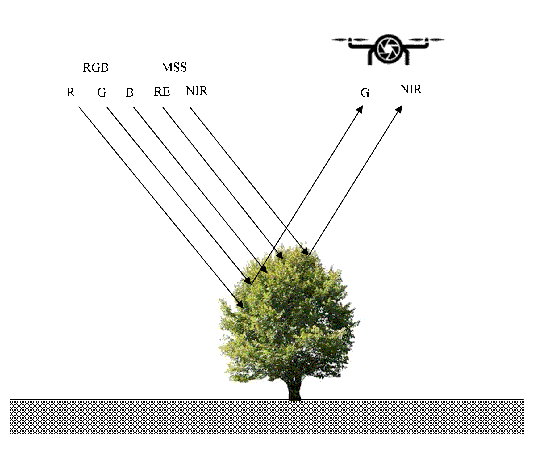
Green Normalized Difference Vegetation Index is similar to NDVI uses visible band-green instead of band-red (Sankaran et al., 2015). Band-INR and G have good abilities to estimate the density and intensity of vegetation cover using solar radiation (Wahab et al., 2018). Reflectance in band-G is more sensitive to plant leaf Chlorophyll and plant health (Wahab et al., 2018). Burke and Lobell (2017) pointed that Band-G is more useful to capture the disparity in nutrient deficiency and therefore crop yield. Therefore, this index is more sensitive to wide range of Chlorophyll and efficient for vegetation analysis than the Normalized Difference Vegetation Index (NDVI) (Gitelson and Merzlyak, 1998). Wahab et al. (2018) have calculated the GNDVI for estimation of vigor and yield of Maize crop. It also shows stronger relation with drought stressed and non-stressed condition crops. Marcial-Pablo et al. (2018) reported superiority of GNDVI for vegetation fraction analysis.
Further, Marino and Alvino (2019) have used Soil-adjusted vegetation index (OSAVI) for estimation of variation in vegetation cover of wheat for yield analyses. Leaf Water Index (LWI) and Two-Dimensional Smoothing Kernels also used for this analysis.
3.5.4 Combinations of Indices (COI)
Some of the researchers have combined RGB indices for detection and estimations of AGB above ground biomass]. Niu et al. (2019) have combined (equation (66)) ExG, ExGR, CIVE and VEG for this purpose as:
\(COI = 0.25 × ExG + 0.3×ExGR + 0.33× CIVE + 0.12 ×VEG\) (65) after Niu et al. (2019)
Wan et al. (2018) have suggested combinations of various VIs (RGRI and NDSI (944, 758)) calculated using UAV-based RGB datasets for estimations for flowing numbers of oilseed ripe.
3.5.5 Estimation, Prediction and Classification Techniques
Researchers have used Support Vector Machine (SVM), Point Cloud (PC), Simple Linear Regression (SLR), Simple Exponential Regression, Random Forest (RF), Partial Least Squares Regression (PLSR) Model, Digital Vigor Model (DVM), K-means method for classification of UAS based RS images for different uses (Table 4).
Table 4. Estimation, Predictions and Classification techniques
|
Technique
|
Data
|
Authors
|
Applications
|
|
Simple Linear Regression (SLR)
|
RGB (3 bands)
MSS (5 bands)
|
Li et al. (2019)
Jiang et al. (2019)
Guo et al. (2019)
|
Estimation of LAI using VIs.
Estimation of plant based on using indices.
To calibrate the MSS images in little cloudy and cloudy weather.
|
|
Multiple Linear Regression (MLR)
|
RGB (3 bands)
|
Li et al. (2019)
|
Estimation of LAI using VIs.
|
|
Partial Least Squares Regression (PLSR)
|
RGB (3 bands)
|
Li et al. (2019)
|
Estimation of LAI using VIs.
|
|
Simple Exponential Regression (SER)
|
MSS (12 bands)
|
Jiang et al. (2019)
|
To estimate the AGB of rice crop.
|
|
Random Forest (RF)
|
RGB (3 bands)
|
Li et al. (2019)
|
Estimation of LAI using VIs.
|
|
Principal Component Regression (PCR)
|
RGB (3 bands)
|
Li et al. (2019)
|
Estimation of LAI using VIs.
|
|
Support Vector Machine (SVM)
|
MSS (5 bands)
|
Javan et al. (2019)
Li et al. (2019)
Durfee et al. (2019)
|
To detect the tree and non-tree objects.
To detect the Greening disease of citrus trees.
Estimation of LAI using VIs.
Canopy classification over a watershed.
|
|
Point Cloud
|
RGB (3 bands)
MSS (5 bands)
|
Themistocleous (2019)
Jiang et al. (2019)
|
To prepared the DEM.
To estimate the TIN based structural aspects of the rice plots.
|
|
Universal Calibration Equation
|
MSS (6 bands)
|
Guo et al. (2019)
|
To calibrate the MSS images in little cloudy and cloudy weather.
|
SVM is classification technique widely used for detection of disparity, land, visitation (plants, crops), etc. (Javan et al., 2019). Javan et al. (2019) have used SVM to detect non-tree space within a plantation (Citrus trees), healthy and diseased trees. Durfee et al. (2019) have used this technique for classification of vegetation over a watershed.
Point cloud technique was used for preparation of DEM using ERGBVE (Themistocleous, 2019). Point cloud data was used to acquire TIN structures of rice plots in Switzerland based on UAV data (Jiang et al., 2019). This method was used for estimation of plant height for calculation of AGB of maize (Niu et al., 2019). Park et al. (2019) have used statistical techniques: mean, median and standard deviation for detection of leaf cover of individual tree using RGB Chromatic Coordinates, excess green, green vegetation, non-photosynthetic indices, etc. Kerle et al. (2020) have showed applicability of 3D point clouds for highly detailed and accurate scene reconstruction to recognize the features.
Simple Linear Regression (SLR) was used of AGB of rice using multiple indices, TIN based structural feature of plots, meteorological data (Jiang et al., 2019). Simple Exponential Regression (SLR) was used of AGB of rice using multiple indices, TIN based structural feature of plots, meteorological data (Jiang et al., 2019).
Buchaillot et al. (2019) have reported better performance of multivariate regression models calculated based on RGB indices for estimations of agronomic parameters. Further, they have calculated grain Yield Loss Index (GYLI) for analysis of variability in crop productions. Fathipoor et al. (2019) have established Partial Least Squares Regression (PLSR) Model using plant height estimated using AUV-RGB based DEM for estimation of crop yield in Iran.
Jiang et al. (2019) have used Random Forest (RF) method for combing the UAV based MSS, structural and metrological data for estimation of AGB of rice crop. Wan et al. (2018) have used this technique for prediction of flower number using UAV-RGB data for oilseed rape. Oliveira et al. (2019) have reported better performance of RF than multiple linear regression calculated from RGB and hyperspectral datasets for estimation and validation of grass. Further, Digital Vigor Model (DVM) has been obtained from Digital Surface Model (DSM) and Digital Terrain Model (DTM) established base on AUV-RGB images (Vanegas et al., 2018). Wan et al. (2018) have used K-mean method for identification of flower coverage area of oilseed rape.
One-tailed Z-test was used to test the significance of relationship between VIs and study objects. Yeom et al. (2019) have conducted this test to find the significance of VIs difference with tillage and non-tillage treatment in agriculture.
Accuracy of estimated results has been achieved more than 95% using UAV remote sensing technique. Javan et al. (2019) have been detected and classified diseased Citrus trees at more than 95% accuracy.


 ,
Ajaykumar Kadam 2
,
Ajaykumar Kadam 2