Keywords

Coastal aquifers , Hydraulic conductivity , Porosity , Transmissivity , Resistivity sounding , Maharashtra

1 . INTRODUCTION

Groundwater is the most prominent natural resource for human life. Excessive groundwater withdrawals have caused encroachment of seawater into the fresh water regions of coastal aquifers, resulting in a worldwide seawater intrusion problem (Werner et al., 2013). Due to rapid growth in population and agriculture, the exploitation of groundwater resources is expanding globally and therefore a cumulative need is required in the field of groundwater management especially in ecologically affected areas. This is more essential due to saline water ingress into coastal aquifers, causing serious concerns in terms of both environmental and economic impacts (Werner, 2010; Shi and Jiao, 2014). In view of this fact, assessable description of the aquifers has become important in order to address most of the hydrological and hydrogeological problems. Formation factor (F_a), porosity (ϕ), hydraulic conductivity (k) and transmissivity (T) are the fundamental properties describing the subsurface hydrology. Usually hydraulic parameters of the aquifers are calculated from pumping tests. However, it is very expensive and time consuming to drill the wells at every location. Besides, the pumping test method yields results appropriate only to a small section of the aquifer. Therefore, better parameter characterization methods are adopted to study the aquifer parameters, especially in hard rock regions.

Surface geophysical methods may contribute substantially towards aquifer characterization. Geoelectrical method, especially the Vertical Electrical Sounding (VES) is a relatively economical, quantitative and non-invasive technique used for locating sites/depths for groundwater exploitation. Besides, it is used as an effective tool for ascertaining the subsurface geological framework of an area to solve or detect the hydrological, geological and geo technical problems (Ward, 1990). The potential benefits of this method in hydrogeological site characterization and aquifer mapping have been stated in numerous studies (Kelly, 1977; Huntley, 1986; Niwas and de Lima, 2003; Cassidy et al., 2014; Das et al., 2016). It is used routinely for aquifer zone delineation and evaluation of the aquifer characteristics. Since a correlation exists between hydraulic and electrical properties, as both properties are related to the pore space structure and heterogeneity (Rubin, 2003), an integration of aquifer parameters calculated from boreholes and surface resistivity parameters is a viable solution to estimate the hydraulic parameters.

Several investigators have characterized and estimated aquifer properties from electrical sounding data in different geologic environments (Batte et al., 2010; Majumdar and Das, 2011; Sikandar and Christen, 2012; Asfahani, 2012; Niwas and Celik, 2012; Nwosu et., al 2013). Soupious et al., (2006) used vertical electrical sounding (VES) data and Dar-Zarrouk (DZ) parameters and suggested a relationship between transverse resistance and the transmissivity of aquifers in Keritis Basin in Chania (Crete-Greece). In these studies several mathematical equations and correlations were developed to estimate hydraulic aquifer properties from surficial electrical data. However, Sattar et al., (2016) are of the view that these estimations are area specific and likely to change in different geologic provinces.

A relation between the aquifer intrinsic permeability and formation factor to estimate transmissivity from borehole resistivity measurements was established by Croft (1971). However, Worthington (1975) obtained an inverse relation between the formation factor and inter-granular permeability. Kelly (1977) established an empirical relation between aquifer electrical resistivity and aquifer hydraulic conductivity and a semi-empirical relation between the aquifer formation factor and hydraulic conductivity. In the present study, an attempt has been made to ascertain the relationship between aquifer and geoelectrical properties in combination with hydro-geochemical information in coastal area of Sindhudurg district, Maharashtra which will improve the characterization of aquifer parameters in the coastal region.

2 . STUDY AREA AND GEOLOGICAL ATTRIBUTES

The study area is a narrow strip between the Sahaydri ranges and Arabian Sea extending from latitude 16º N to 16.5º N and longitude 73º E to 73.74º E in Sindhudurg district, Maharashtra, India (Figure 1). Different types of rock formations exist in the study area having varied petro-physical properties, imparting different capacities to store and transmit water. Geologically the study area exposes rocks ranging from Archean to Quaternary period. The Archean granites and gneisses are medium to coarse grained and consists of quartz, hornblende, orthoclase biotite and microcline (CGWB, 2014). Dharwarian meta-sediments (Archean), Kaladgi formation (Precambrian), Deccan Trap lava flows (Upper Cretaceous to Lower Eocene age), Laterite (Pleistocene) and Alluvial deposits (Recent to Sub-Recent) are the water bearing formations in this district (CGWB, 2014). The Kaladgi formation occurs in limited patches and thus does not form potential aquifer in the area. The Alluviums has limited areal extent found mainly along the coast. As the primary porosity is insignificant in the Deccan trap basalts, secondary porosity due to jointing and fracturing plays an important role in groundwater movement.

Figure 1. Location map of the study area showing the geochemical sampling points and the vertical electrical sounding (VES) points (after GSI, 2000).

The district falls in humid and high rainfall zone. The annual rainfall ranges from 2542-3938 mm from North to South (CGWB, 2014). Fluctuations in the temperature with an average annual rainfall of around 3,287 mm are not significant in this coastal region wherein the mean daily maximum temperature is 32.7 ºC and the mean daily minimum temperature is 18.7 ºC, while the relative humidity is greater than 60%. Groundwater level in the study area varies from 2 to 20 m below ground level (CGWB, 2014).

3 . MATERIALS AND METHODS

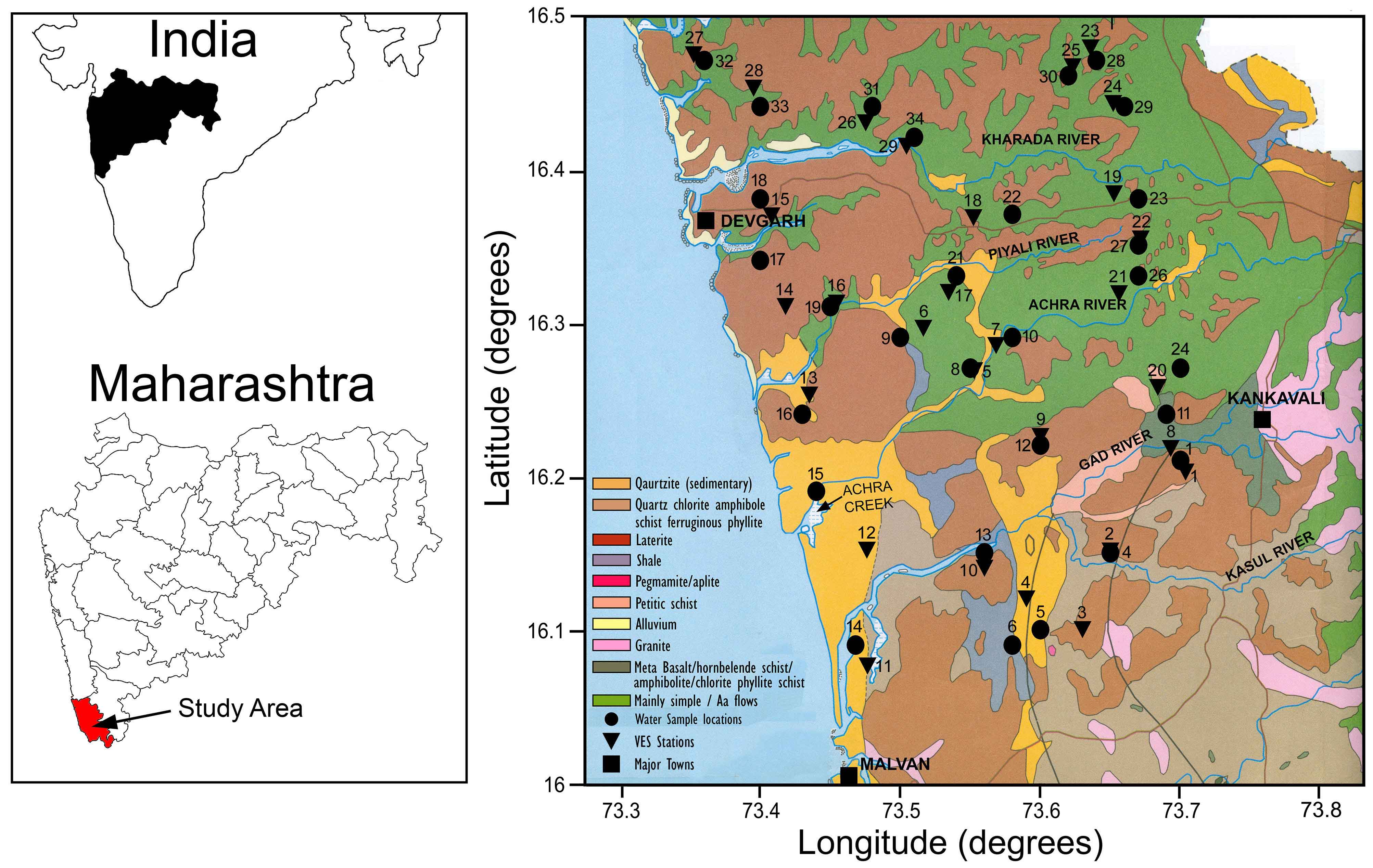
In this work, 29 Schlumberger VES were considered from the study area (Figure 1) with a maximum current electrode half-spacing (AB/2) of 100 m. Resistivity measurements was carried out using a digital signal-enhancement resistivity meter (IGIS make, Hyderabad). All the 29 VES stations were conducted close to pre-existing wells. A total of 29 water samples (Figure 1), collected from the respective dug wells and boreholes were used for the determination of pore-water resistivity.

The calculated apparent resistivity data were inverted to construct true geological model of the subsurface using IPI2WIN software (Bobachev, 2003). The aquifer model parameters (layer resistivity and layer thickness) for all 29 VES sites were used for estimating the hydraulic parameters. The resolution of resistivity data interpretation is often hindered due to some geophysical similarities in the behavior of different geomaterials. In view of this, secondary geophysical parameters (\(T_r\), transverse resistance and \(S\), longitudinal conductance) (also known as Dar Zarrouk, (D-Z) parameters) are used to minimize these uncertainties (Maillet, 1947).

Several relationships between transverse resistance (\(T_r\)), longitudinal conductance (\(S\)), transmissivity and hydraulic conductivity have been established by different workers (Ungemach et al., 1969; Kelly, 1977;  Mazáč et al., 1985; Niwas and Singhal, 1985; Huntley, 1986; Mazáč et al., 1988; Boerner et al., 1996; Christensen and Sorensen, 1998; Rubin and Hubbard, 2005; Soupis et al., 2007). These relationships were essentially site specific.

In order to acquire quantitative information on groundwater flow and pollutant transport modeling, evaluation of hydraulic properties of any given aquifer system is of prime importance. These aquifer hydraulic properties are obtained either from conventional pumping tests carried out in wells or from laboratory core samples experiments (Soupios et al., 2007). In the present study, using the Kozeny–Carman–Bear (KCB) equation (Domenico and Schwartz, 1990), hydraulic conductivity values were estimated. The porosity (\(\phi\)) and other petro physical parameter required in KCB equation was calculated using Archie’s empirical law (Archie, 1942).

\(\rho_o=a\rho_w\phi^{-m}\)              (1)

where, \(\rho_o\), \(\rho_w\), \(a\), \(m\) and \(\phi\) are bulk resistivity, pore-water resistivity, pore geometry factor, cementation factor and fractional porosity, respectively.

Equation 1 is applicable to clay free medium only and thus \(\frac{\rho_o}{​​\rho_w}\)  ratio is known as the intrinsic formation factor (\(F_i\)). Accordingly, equation 1 could be re-written as (equation 2),

\(\phi=e^{\frac{1}{m}In(a)+\frac{1}{m}In(\frac{1}{F_i})}\)          (2)

The coefficients \(a\) and \(m\) is usually determined from core samples for each site under investigation. But, due to unavailability of core samples in the study area, the values for \(a\) and \(m\) reported in published literature was used to obtain porosity values.

Worthington (1993) advocated three different expressions to compute intrinsic formation factor corresponding to the porosity of samples from different sites. A fourth expression is given by Jackson et al., (1978) and De Lima and Sharma (1990) where the coefficient \(a\) has the value of 1 while \(m\) varies from 1.3 to 2.5. As mentioned earlier, Archie’s formula (equation (1) and (2)) is applicable only for clay-free, clean, consolidated sediments and therefore any departure from these assumptions from actual field data make the equation invalid. Worthington (1993) proposed that for unclean, clayey and shaley sands and a mixture of sand/ gravels, some remedial measure for clay conductivity is required and thus in the present study, the coefficient \(a\) has the value of unity while \(m\) is taken as 2.5.

Several researchers have given different models which are basically derived empirically using the notion of parallel conductor (Patnode and Wyllie, 1950; Winsauer and McCardell, 1953; Waxman and Smits, 1968; Sen et al., 1988). In the present study, the Archie’s equation was modified using the Waxman–Smits model (Vinegar and Waxman, 1984) which relates the apparent formation factor (\(F_a\)) (which is the ratio of bulk resistivity to pore-water resistivity) and intrinsic formation factor (\(F_i\)), after taking into account the shale effects. According to Worthington (1993),

\(F_a=F_i(1+BQ_V\rho_w)^{-1}\)              (3)

where, \(BQ_V\)  term is related to the effects of surface conduction due to clay particles. In case of surface conduction effects are non-existent, the apparent formation factor (\(F_a\)) is equal to the intrinsic formation factor (\(F_i\)). Rearranging the terms in equation 3, we obtain,

\(\frac{1}{​​F_a}=\frac{1}{​​F_i}+(\frac {BQ_V}{F_i})\rho_w\)            (4)

Consequently, plotting the pore-water resistivity ( \(\rho_w\) ) as a function of  \(\frac{1}{​​F_a}\)  enables us to get the corrected \(\frac{1}{​​F_i}\)  values. The relation theoretically results in a straight line and \((\frac {BQ_V}{F_i})\)  is denoted by slope (Das et al., 2016). The value of the corrected formation factor thus obtained will subsequently facilitate us to estimate porosity via equation 2. The above approach is followed by using bulk resistivity \(\rho_o\)  obtained from the one-dimensional (1D) resistivity inversion coupled with pore-water resistivities measured from wells near VES stations. However, some uncertainty prevails here due to fact that a few of the wells are at some distance away from the corresponding VES points.

Table 1 gives the resistivity values obtained from 1D inversion and the calculated apparent formation factors. By applying least square best fit linear approach of the individual groups of the dataset between \(\frac{1}{​​F_a}\) and pore-water resistivity (\(\rho_w\)), the intrinsic formation factor is obtained which ranges from 0.000318 to 0.0389 (Table 1). The porosity values can now be estimated by substituting the \(\frac{1}{​​F_i}\)  values, and the \(a\) and \(m\) values are taken as 1 and 2.5, respectively in equation 2.

In order to determine the hydraulic conductivity (\(k\)), KCB equation 5 (Soupis et al., 2007) was used as,

\(k =(\frac{\delta_wg}{\mu})\cdot(\frac{d^2}{180})\cdot(\frac{\phi^3}{{(1-\phi})^2})\)            (5)

where, \(d\) is the grain size (0.01 cm) (Soupis et al., 2007), \(\delta_w\)  fluid density (1000 kg/m³), \(\mu\)  and \(g\) are dynamic viscosity of the fluid (0.0014 kg/ms) and acceleration due to gravity (Fetter, 1994), respectively.

The secondary geophysical parameters of significance in this study are longitudinal conductance \(S\), transverse resistance \(T_r\) and electrical anisotropy \(\lambda\) which are given after (Zohdy, 1974) for \(n\)-layer as,

Longitudinal conductance,   \(S=\sum_{i=1}^{n} (\frac{h_i}{\rho_i})\)    (6)

Transverse resistance, \(T_r=\sum_{i=1}^{n} ({h_i}{\rho_i})\)        (7)

where, \(h_i\)  is the saturated thickness of each layer, \(\rho_i\)  is the true resistivity of each layer.

Coefficient of anisotropy  \(\lambda = \sqrt{( \frac {\rho_t}{\rho_l}) }\)    (8)

where, \(\rho_t\)  and \(\rho_l\)   are the average transverse resistivity and average longitudinal resistivity, respectively.

The rate of flow of the aquifer is called the transmissivity (\(T\)), which can be calculated by the following equation

\(T=k*h\)         (9)

where, \(k\) is hydraulic conductivity of the aquifer which is obtained from equation 5 and \(h\) is thickness of the aquifer derived from the 1D resistivity values of the VES points. These enable us to derive a relation between transverse resistivity and transmissivity, to be discussed later. Also the relation between porosity and electrical anisotropy is obtained in order to understand the functional corresponding relationship.

4 . RESULTS AND DISCUSSION

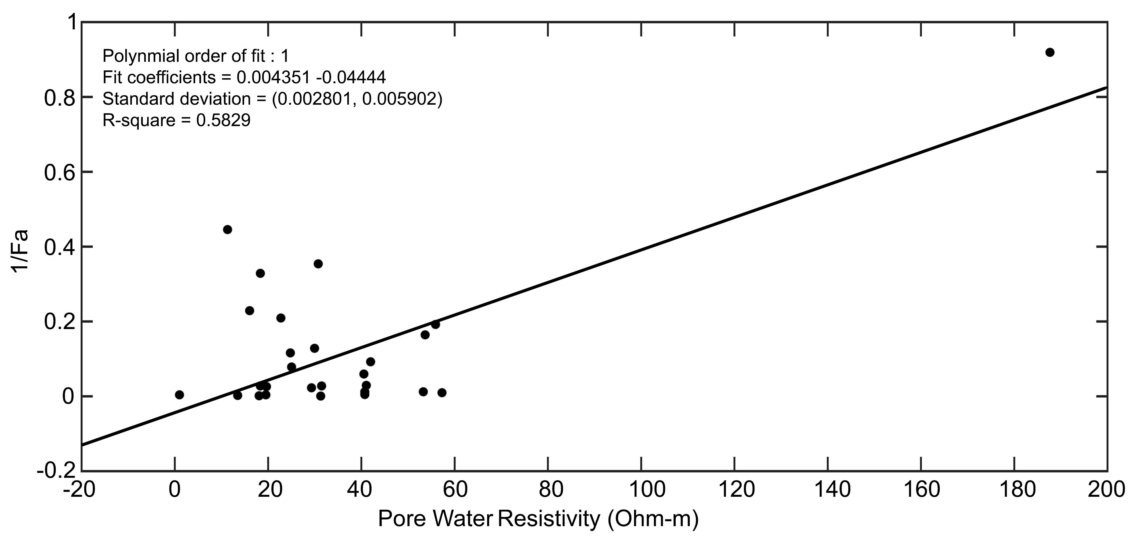
As mentioned earlier, the correlation between pore-water resistivity ( \(\rho_w\) ) and inverted formation factor ( \(\frac{1}{F_a}\) ) is obtained in order to calculate the intrinsic formation factor ( \(F_i\) ) (Figure 2). This revealed a straight 

Figure 2. Determination of the intrinsic formation factor

line with slope 0.004 and intercept value of -0.044 and giving the coefficient of determination of 0.583. The correlation plot suggests that as ρ_w increases, the formation factor (\(F_a\)) decreases which satisfy the Archie’s equation.

In the present work, the spatial variation of aquifer parameters were determined using the ordinary kriging technique, which is a linear stochastic method using semi-variogram model fitting schemes so as to estimate values at unknown sites using the values at known sites (Das et al., 2016).

4.1  Spatial Distribution of Aquifer Thickness

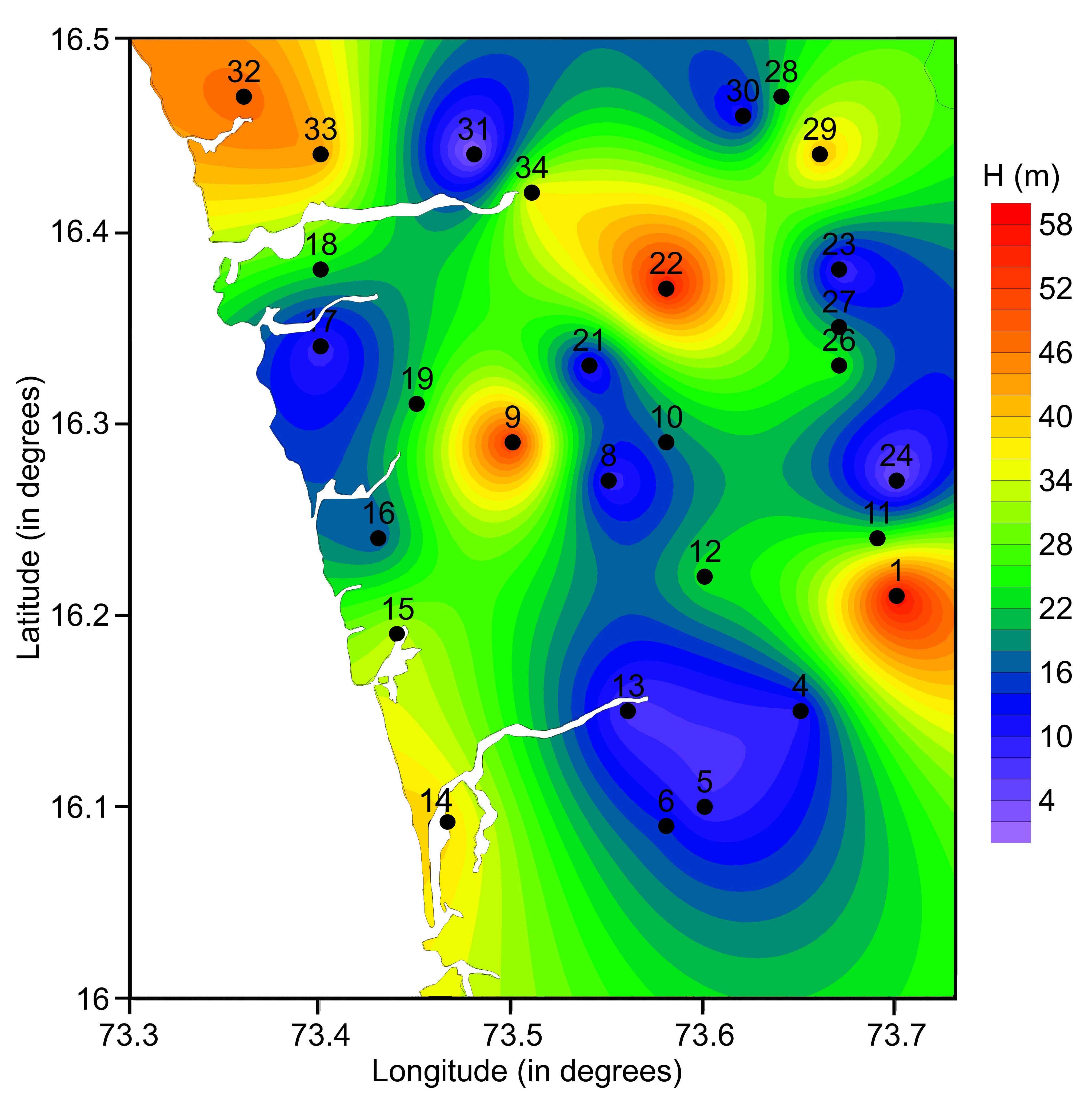
Figure 3 represents the spatial variability of the aquifer thickness, which is extracted from the VES location (Table 1). The aquifer thickness ranges from 0.67 to 59 m in the study area. The low aquifer thickness below 5 m was observed at locations 24 and 31. Higher aquifer thickness greater than 30 m were seen along the coastal sites 14, 15, 32 and 33, central region (9, 22 and 29) and at site number 1 to the East, due to undulating topography. Thickness of the aquifer plays a very important role in understanding the hydraulic parameters of the study area. Moderately thick aquifers seen mainly in the Northwest and central part of the study area may represent productive aquifer zones. In the basaltic terrain, groundwater occurs under unconfined conditions in the phreatic zone up to a depth of 15-20 m in the weathered zone, fractures and joints in the massive unit and weathered/fractured vesicular units.

Figure 3. Spatial variability map of aquifer thickness (H).

4.2  Spatial distribution of porosity

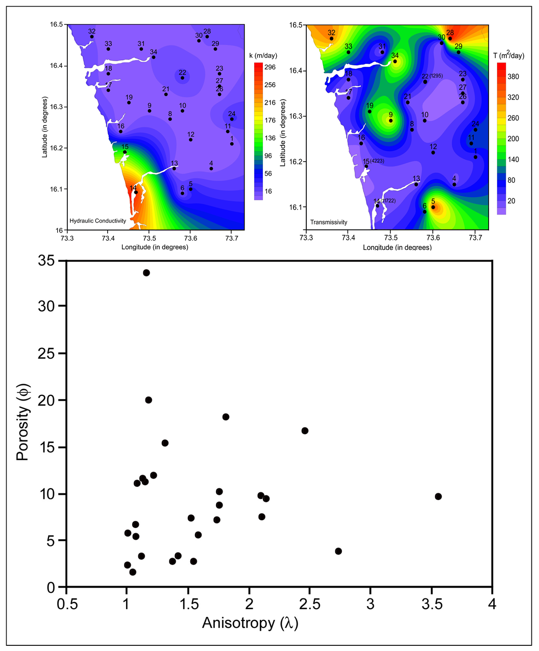
The spatial distribution map of the porosity is shown in Figure 4. Porosity is a very important parameter in the aquifer characterization and groundwater management. Evidently the productivity of an aquifer depends on the geological characteristics of the lithological units and porosity. The aquifer porosity in the study area ranges from 1.5 to 33% (Table 1). Generally the porosity values reported earlier from the southern part of the study area ranges up to about 30% (Das et al 2016). Porosity values >20% are observed at locations 5, 14, 15, 22, 24 and 28. Very high porosity values (>27%) are observed at south-western part at wells 14 and 15, since this part of the coastal tract comprises of alluvium formation of fine grain and un-lithified sediments (Figure 4), resulting in high porosity content.

Figure 4. Spatial variability map of porosity.

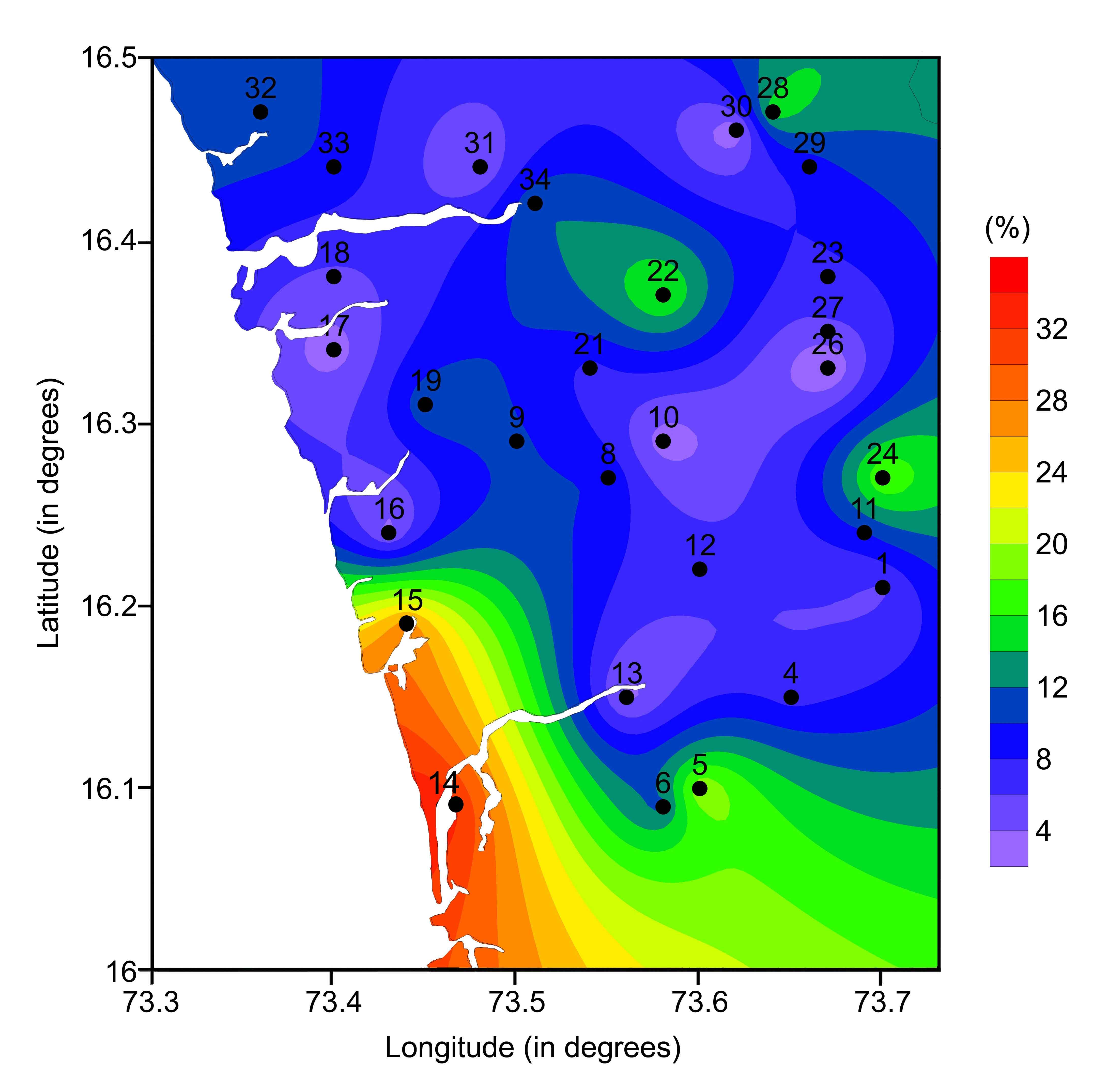
4.3  Spatial Distribution of Hydraulic Conductivity

The spatial distribution map of the hydraulic conductivity (Figure 5) is a vital parameter of aquifer systems as it strongly affects fluid flow by creating flow barriers or preferential flow paths. The estimated hydraulic conductivity (\(k\) is shown in Table 1, which ranges from 0.014 to 293 m/day. High \(k\) values (>100 m/day) are observed in the coastal part at sites 14 and 15. This part also revealed high porosity values indicating that it is underlain by good aquifer materials and thus making the area a good prospect for groundwater. The \(k\) map further suggests moderately high values in the Southern, Eastern and Central parts of the study area, which are characterized by high porosity. This suggests that cracks and inter-connected pores play a major role in the permeability to determine the conductivity of fractured rocks (Francis, 1981; Schwartz and Zhang, 2004).

Figure 5. Spatial variability map of hydraulic conductivity.

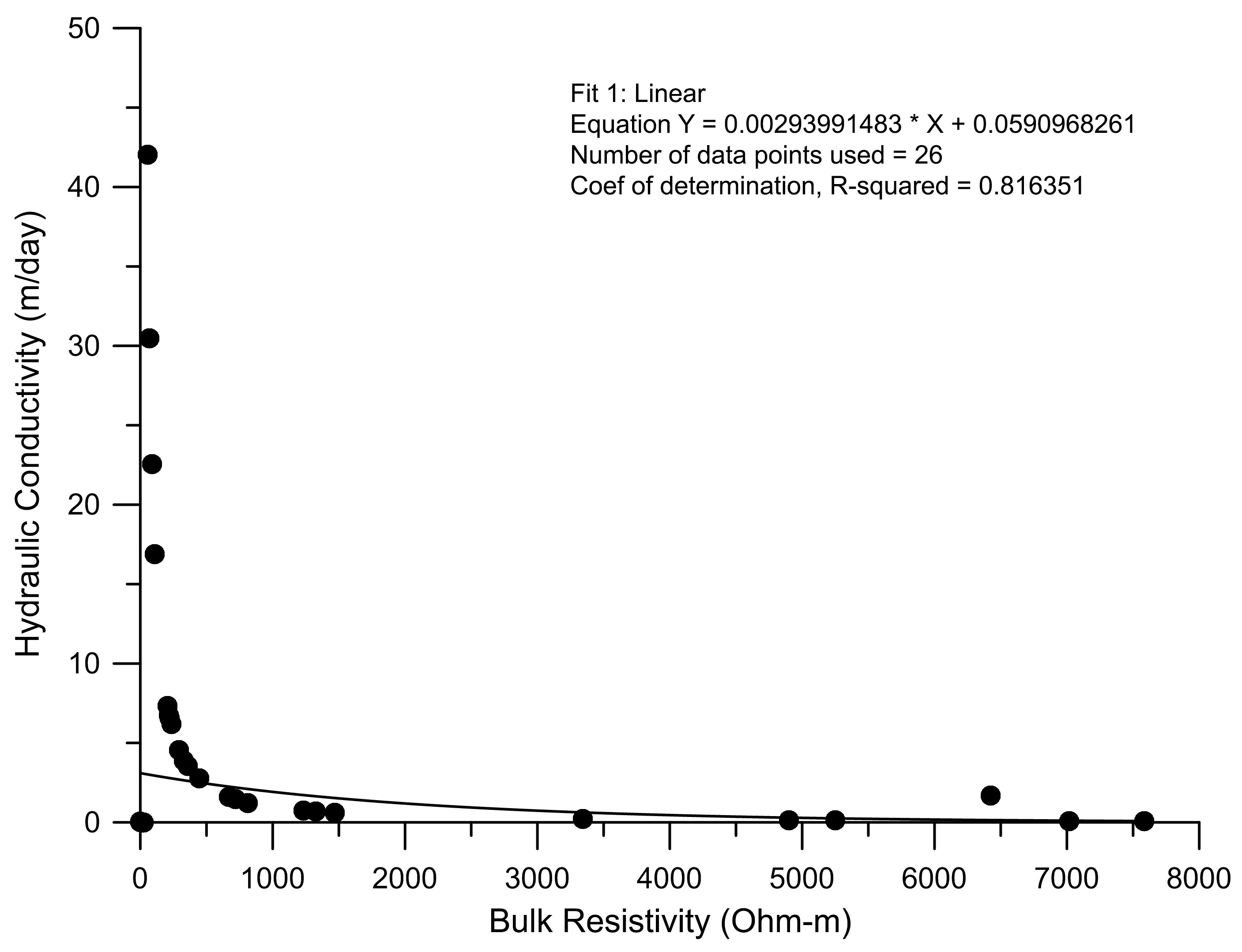
The correlation between bulk resistivity and hydraulic conductivity is usually considered for clean saturated sediments, whose natural fluid characteristics are constant (Henriet, 1975). The correlation plot (Figure 6) reveals a negative relation between these two parameters suggesting that the hydraulic conductivity exponentially decreases with increasing bulk resistivity due granitic gneiss and lateritic formations (Das et al., 2016). Rock properties are influenced by the permeability including particle size, its packing and distribution and degree of lithification. In the present study, the increase in hydraulic conductivity with decreasing bulk resistivity is attributable to the better inter-connectivity of fracture network in crystalline hard rock.

Figure 6. Correlation plot between bulk resistivity and hydraulic conductivity.

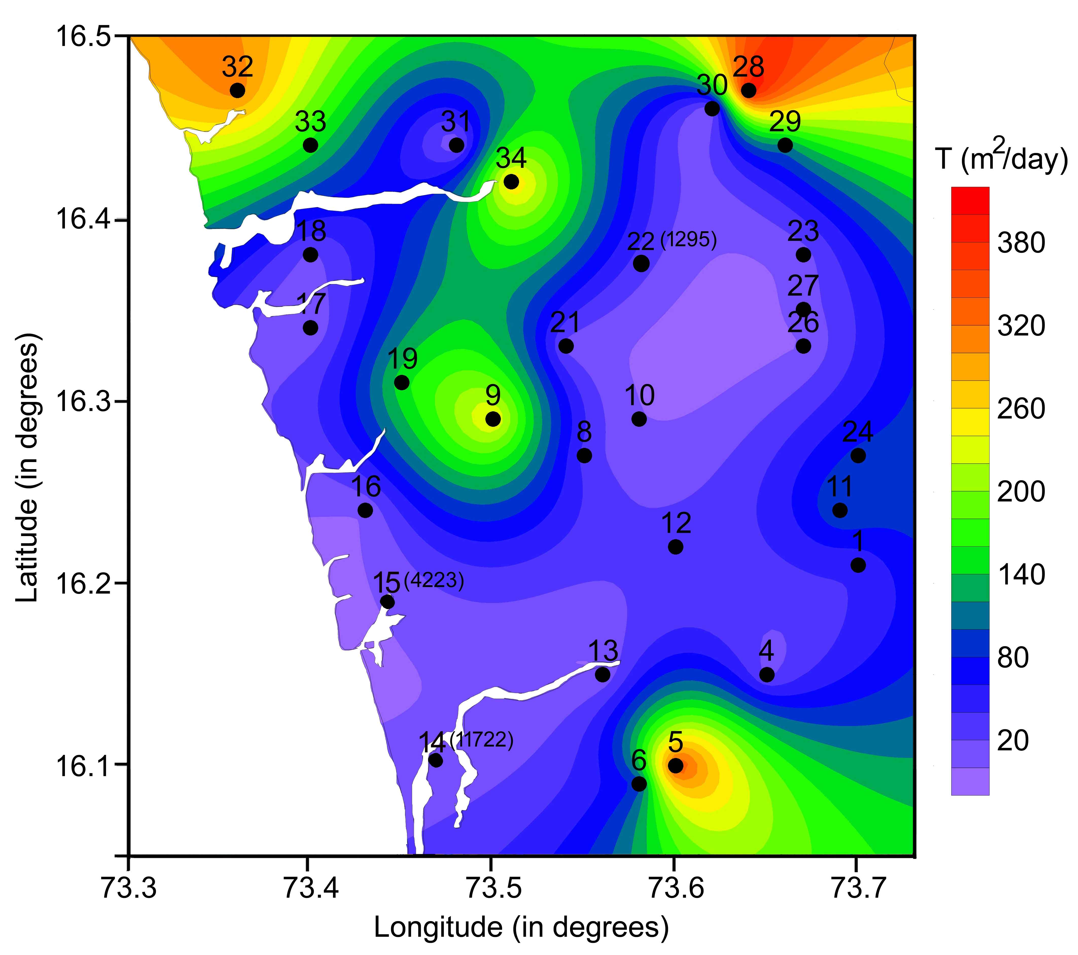
4.4  Spatial Distribution of Transmissivity

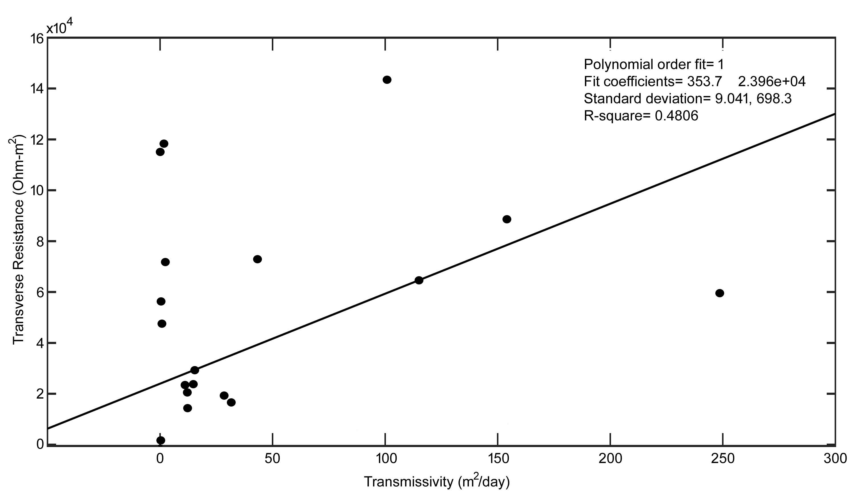
Transmissivity (\(T\)) is defined as the rate of flow under a unit hydraulic gradient through a unit width of aquifer of given saturated thickness. It is the most important parameter in hydrogeological environment because the higher transmissivity, more productive is the aquifer. In the present study, the T value ranges from 0.142 to 11722 m²/day (Table 1). Higher values are observed at station 14 (11722.4 m²/day) and station 15 (4222.9 m²/day) (Figure 7). Station 22 in the central part of the study area shows \(T\) value of 1294.9 m²/day. These three sampling points are not considered in interpretation as the very high T value tends to mask the effects of other features in its vicinity. However, it is marked on the map (Figure 7) and the \(T\) values are given in parenthesis. These three stations have more aquifer thickness and hydraulic conductivity, thereby leading to higher transmissivity. Pumping test results of aquifer parameters from the study area suggests that the transmissivity ranges from 5.6 to 375 m²/day (CGWB, 2014). It can be observed from the present study that apart from samples 14, 15 and 22 all other samples are comparable with the transmissivity values given by CGWB (2014). Also the spatial variation map of transmissivity (Figure 7) reveals a positive correspondence with hydraulic conductivity almost over the entire study area in general and at Western part in particular.

Figure 7. Spatial variability map of transmissivity (T).

4.5  Correlation between Transmissivity and Transverse Resistivity

As mentioned earlier, transmissivity is an indication of the ability of a layer of known hydraulic conductivity to transmit fluids through its entire thickness. It has been advocated that the transmissivity of an aquifer is directly proportional to its transverse resistance (Henriet, 1975; Ward, 1990). In order to check the accuracy of the computed hydraulic conductivity values determined from the resistivity values, an attempt is made to obtain a relationship between transmissivity and transverse 

resistance. The transverse resistance value ranges from 586 to >700000 Ω -m² (Table 1). High transverse resistance values are usually associated with zones of high transmissivity and hence highly permeable to fluid movement. A positive relation is obtained between transmissivity and transverse resistance and the best fit regression line is shown in Figure 8.  This suggests that the prospective aquifer zones in the study area increases with increasing transverse resistance. These are presumably due to changes in hydraulic conductivities and electrical anisotropy, in addition to the disparity in lithology, mineralogy, grain size, size and shape of the pores and pore channels (Salem, 1999).

Figure 8. Relation between Transverse Resistance, TR (Ω -m2) and Transmissivity, T (m2/day).

4.6  Correlation between Electrical Anisotropy and Porosity

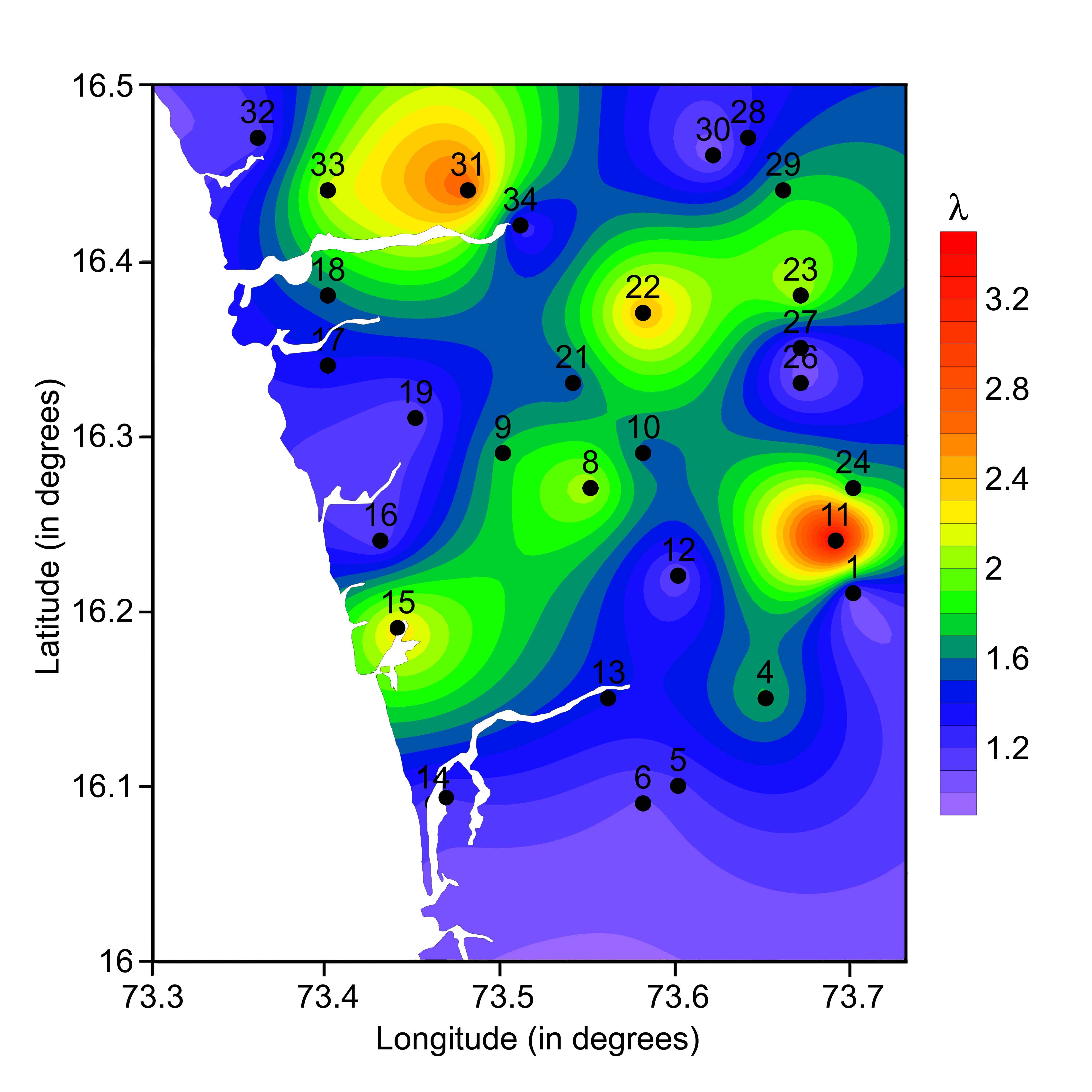
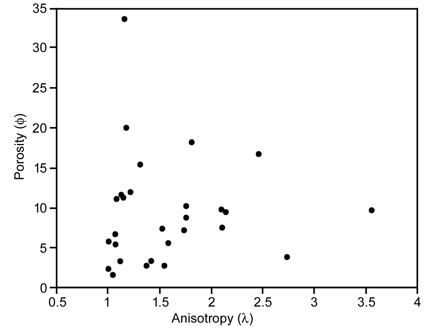
Fractures in rocks are important pathways for groundwater flow and contaminant migration. Groundwater flow through a fracture network is strongly influenced by anisotropy resulting from the geometry of the fractures (Slater et al., 2006), since both current flow and groundwater are channeled through fractures in the rock. It is reported by Zohdy (1974) that the coefficient of anisotropy (λ) is generally 1 and seldom exceeds 2 in most of the geological conditions. Keller and Frischknecht (1966) are of the view that as the hardness and compaction of rocks increases, \(\lambda\) also tends to increase, which are thus associated with low porosity and permeability.

Electrical anisotropy in the study area varies from 1-3.55 (Table 1). The coefficient of anisotropy is not uniform in all directions and is observed to increase from SW to NE and also from SE to NW (Figure 9), thus playing a major role in fracturing. More fracturing towards the NE an SW directions suggest relatively more prospective groundwater zone. Resistivity of subsurface rocks affects both the electrical anisotropy and porosity. Porosity critically depends upon the existence of a petrophysical relationship between geoelectrical properties in an area. An analogy drawn between both these parameters (Figure 10) suggests that about 80% of the sampling sites concentrated within λ values 1-2 reveal higher porosity. This implies that the study area portrays differing extent of saturation zones within the lateritic and basaltic rock formation.

Figure 9. Spatial variability map of electrical anisotropy (λ).

Figure 10. Plot of electrical anisotropy (λ) and porosity.

5 . CONCLUSIONS

An integrated method is presented to estimate the aquifer parameters by using vertical electrical sounding (VES) and hydrochemical data of the coastal region of Sindhudurg district, Western Maharashtra, India. This is very cost effective and quick when pumping test data of the area is unavailable. The relation between bulk resistivity and hydraulic conductivity is established by using VES inverted data and hydrochemical sample analysis. Further, spatial variation of aquifer parameters like transmissivity, hydraulic conductivity, aquifer thickness and porosity was evaluated and contoured using ordinary kriging scheme.

The transmissivity values are vary between 0.142 and 11722 m²/day, which can be attributed to the subsurface inhomogeneity of the sandy silt and lateritic formations in the coastal part of the study area. The high values of transmissivity could be due to the presence of fractured medium saturated with water, suggesting high potential within the water-bearing formation. The T values observed here are corroborating well with the values obtained from pumping test data of CGWB (2014). A positive linear relationship has been obtained between transmissivity and transverse resistance which suggests high permeability formations. The calculated hydraulic conductivity reveals high values (>100 m/day) near the coastal part of the study area. This is due to the increase in sandy silt thickness and also due to high porosity values because the grain size is very fine. The high porosity also advocates that the geological medium could be fractured and indicative of high potential water-bearing formations. The regions of high porosity also corroborates with the regions of electrical anisotropy (between 1 and 2). This suggests the subsurface in homogeniety is due to layers with different resistivity values and also due to fracturing, metamorphism and disseminated ore grains in the rocks.

From the foregoing it can be surmised that geoelectrical sounding technique can be successfully integrated with hydro geochemical parameters for evaluating the hydraulic parameters of the aquifer. This scheme is very suitable where pumping tests data is not available and therefore is cost effective and can significantly reduce the amount of test drilling sites. Such studies can thus be implemented for detailed investigation so as to provide rapid complementary data for the assessment of groundwater potential zones especially in hard-rock terrain of the country where resources are meager.

Tables

Figures

Conflict of Interest

Acknowledgements

Abbreviations

References