Predicting the Amount of Fertilizers using Linear Programming for Agricultural Products from Optimum Cropping Pattern

1. Introduction

Over the centuries, surface and groundwater have been the important resources for agriculture, industry and urban areas. Water resources in each country is a source of income and water has been regarded as an economical resource (Rogers et al., 2002; Othman et al., 2012). Water shortages directly and indirectly effect on sectors such as water resources management, planning, water supply and especially in cropping pattern (Heydari, et al., 2013). Due to The resource constraints and increasing demand for water in different areas such as drinking, agriculture, industry and environmental issues, led to the decision makers seriously think about sustainable development, optimal use of resources and analysis on it (Othman et al., 2012; Othman, et al. 2014).

During the last decades, optimization models have been used widely in water resources systems planning and management. The main focus of studies was on developing tools to help decision making in water resources planning and development (Othman et al., 2012). The optimal answer for a programming problem is a plan that shows the maximum or minimum amount of the objective while satisfying all constraint (Othman et al., 2012). Note that maximization problem can convert to the minimization problem by multiplying 

the objective function in the minus one and vice versa (Heydari, et al., 2015).

Aside from the optimum cropping pattern, the policy makers, employers and managers in the agricultural sector are very interested to be informed about the amount of agricultural inputs (such as fertilizers) before the agricultural activities commence. This knowledge helps them to know the funding requirements as well as storing, maintaining and managing the agricultural process.

Most of the resources, restrictions, aims and sensitivities of these kinds of matter that can be compiled with developing models based on linear programming are considered and determined as an optimal cropping pattern. Here are examples of some studies that have been conducted on determining an optimal cropping pattern especially with the help of computer software and programming models. Omoregie and Thomson (2001) have studied the competition in oilseeds production method using linear programming in Nigeria. The results of this study are concerned that transportation costs as the main factor in reducing the profitability of oilseed production. Singh et al. (2001) have used linear programming to optimize cropping pattern in Pakistan.

Maximizing the net income was the objective function. Total available water and land during different seasons, the minimum area under wheat and rice for local food requirements, farmers’ socio-economic conditions and preference to grow a particular crop in a specific area were constraints. Based on the results, the cultivation of wheat was the most profitable crops. Doppler et al. (2002)  have provided the optimal pattern of water and cultivation together for the Jordan valley using the approach of MOTAD risky planning. Based on the results, it was found that even if the risky considerations are included in the model, the share of cereals will be increased due to the lack of cereals’ price fluctuations in the risky pattern. Francisco and Ali, (2006) have analyzed the interaction and dynamic effects between various production technologies, activities and constraints among vegetable growers in Manila Taiwan. In this study, the minimum variance pattern was used for incorporating the risk.

In recent years, other researchers (Fasakhodi et al., 2010; Montazar et al., 2010; Zeng et al., 2010, Regulwar and Gurav, 2011; Singh and Panda, 2012) have been used linear programming to determine the cropping pattern. The important issue for agricultural managers is to estimate the costs of economic evaluation of projects. They tend to know the implementation cost of the project with almost a good accuracy before  starting the project. The main objectives of this study are to achieve the optimum cropping pattern and estimate the cost of the fertilizer in Khuzestan region. 

The objectives of this study are:

1. To obtain the optimum cropping pattern that supplies the maximum final value of agricultural products with regard to the constraints.
2. To estimate the cost and required quantities of the fertilizer according to the calculated optimum cropping pattern.

2. Material And Methods

2.1 Study Area

Khuzestan State is one of the 31 provinces of Iran (Figure 1). The capital of Khuzestan is Ahvaz and it also covers an area of 63,238 km². Khuzestan has excellent potentials for farming expansion. The abundance of water and fertile soil has caused the area to become suitable land for cultivation such as Wheat, Barley, Husks, Corn, Pea, Lentil, Sunflower, Cotton, Sugar Beet, Watermelon, Cucumber, Potato, Onions, Tomatoes, Canola, Beans, Soya Bean and Rice. The weather of Khuzestan is usually hot (summertime temperatures regularly exceed 40°C) and sometimes humid. While winters are much more cold (sometimes temperature drops below 0°C) and dry.

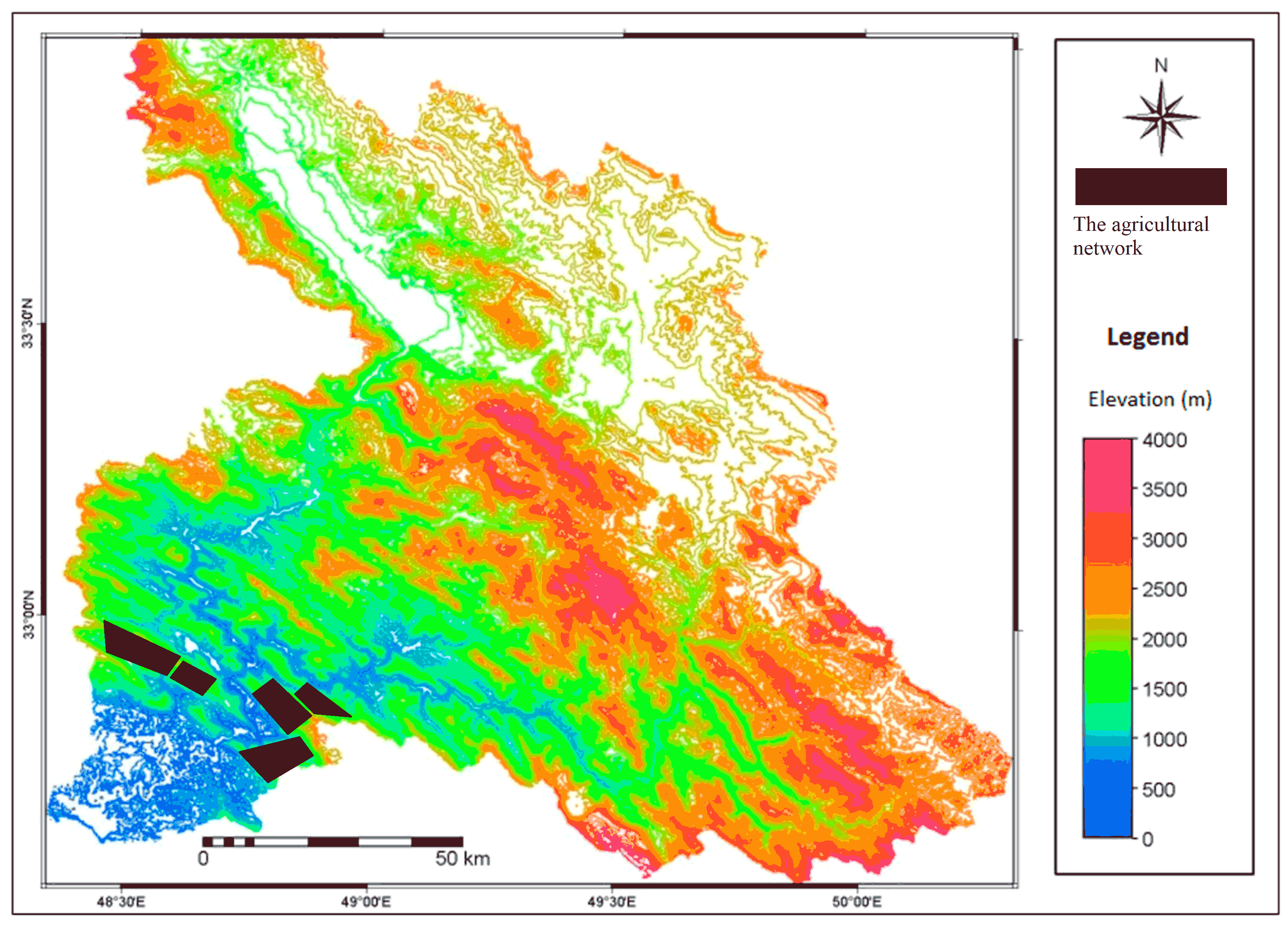
In 2016, only four crops (Wheat, Barley, Sugar Beet and Soybeans) were cultivated in very low levels in the study area.

2.2 Methodology

The methodology is shown in the flowchart (Figure 2). Design cultivated and processes are influenced by many factors that study about that force the designer pattern to collect a wealth of data and information. It is crucial to pay particular attention to the projects’ effective operation to obtain the utmost benefits and satisfaction from all the goals set earlier (Heydari et al., 2015).

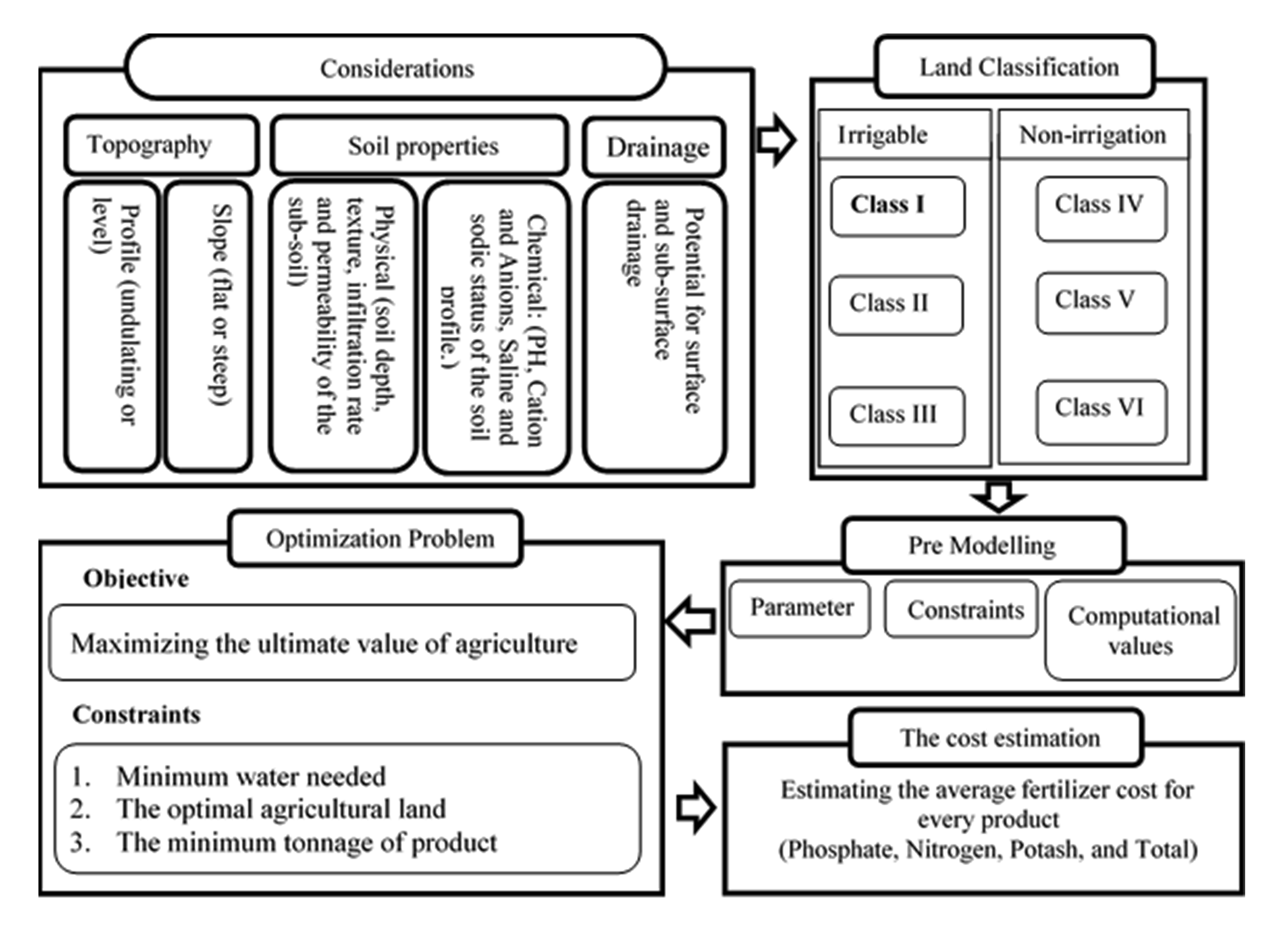
The first requirement in the study of water resources projects in an area is knowledge of water resources and ability to estimate it in the region (Salarian et al., 2013). So the topography, agricultural land, drainage and soil properties of study area were considered and classified into 6 classes. Only 2100 acres of the best farming land (Class I) was studied (Table 1). The volume of assigned water to the described land was about 6 million cubic meters (MCM). 17 agricultural products of the region, including Wheat, Barley, Husks, Corn, Pea, Lentil, Sunflower, Cotton, Sugar Beet, Watermelon, Cucumber, Potato, Onions, Tomatoes, Canola, Beans, Soya bean and Rice were used for this modeling.

Table 1. Soil classes

Classes	I	II	III	IV	V	VI	Total Reported
Karun III downstream (ha)	2100	10600	13400	440	21300	20960	68800
Total (ha) (Khuzestan)	--	--	--	--	--	--	931256
Area (%)	0.23	1.14	1.44	0.05	2.29	2.25	17.93

2.2.1 Pre Modeling

The required data for modeling were prepared in the form of constants, the upper and lower limits values and computational values in the pre modeling phase. Table 2 shows the mentioned data, ( \(∀i=1,2,3,…,17\) ):

Minimum land required for production _i = (Minimum tonnage _i)/(Average production per hectare _i)            (1)                                

Minimum water required to provide the desired capacity_i = (Min land required)_i * (Minimum required water)  (2)

Value per hectare_i = (The product value per ton) _i * (Average production per hectare) _i                                    (3)

Table 2. Inputs*

Agricultural Products		Units	Wheat	Barley	Husks	Corn	Pea	Lentil	Cotton	Sugar beet	Watermelon	Cucumber	Potato	Onions	Tomatoes	Canola	Beans	Soy spring	Rice
Constants	The minimum required water	m3/ha	4340	3730	4180	5060	3940	4630	9160	4710	11850	3800	2970	4530	4625	6590	4930	3220	8890
	Average production per hectare	ton/ha	2.68	2.71	4.25	6.39	1.05	1.2	2.37	42.02	27.69	19.48	29.03	37.18	37.69	2.08	1.67	2.34	4.23
	The product value per tone	1000 Toman	1050	780	850	870	1900	2000	2200	210	374	300	300	200	200	1900	1800	1700	2700
Constraints	Maximum available agricultural land	ha	400	300	40	20	200	200	200	30	40	40	40	40	40	140	200	60	110
	The minimum land required for production	ha	374	185	24	8	57	59	8	2	3	2	3	3	5	72	60	56	95
Computational value	Value per hectare	1000 Toman	2.81	2.11	3.62	5.56	2	2.39	5.21	8.82	10.35	5.84	8.71	7.44	7.54	3.95	3.01	3.97	11.42
	The minimum land required for production	ha	374	185	24	8	57	59	8	2	3	2	3	3	5	72	60	56	95
	Minimum water required to provide the desired capacity	1000 m3	1622.4	688.2	98.3	39.6	225.1	271.2	77.3	9.0	19.0	7.8	10.2	14.6	8.8	475.5	295.2	179.3	840.9

* The data is assumed only for the case study and annual distribution is considered.

2.2.2 Optimization Modeling

The optimization problem had been modeled with the purpose of maximizing the final value of farming and subject to minimum water required, the optimal farming land and the supplying the minimum demand of any agricultural product (equation 4 to 8).

Objective Function:

Maximum Z = Ʃ(Optimal area of agricultural land for production * Value per hectare)_i  \(∀i=1,2,3,…,17 \)           (4)

Constraints:

Minimum water required to provide the desired capacity_i  \(≤\)  the total allocated water   \(∀i=1,2,3,…,17 \)           (5)

The optimal area of agricultural land_i \(≤\)  Maximum available agricultural land _i     \(∀i=1,2,3,…,17 \)         (6)

The optimal area of agricultural land _i \(≥\)  Minimum land required for production _i       \(∀i=1,2,3,…,17 \)      (7)

The minimum tonnage_i \(≥\)  Average production per hectare _i    \(∀i=1,2,3,…,17 \)         (8)

2.2.3 Implementation

The explained model solved through Linear Programming in MS Excel (Solver). Excel includes an effective tool called Solver for optimization problems. The solver can solve the vast majority of optimization problems like linear programming, nonlinear programming and integer programming.

2.2.4 The cost estimation:

The predicted expenses of the fertilizer of farming, including phosphate fertilizer, nitrogenous fertilizer, and potash fertilizer were the last phase. Considering that the objective function determined the best cropping pattern in terms of the number of acres of every crop, we are able to estimate and forecast the cost of the each fertilizer. For this specific purpose, we need to multiply the obtained result of cultivation pattern in hector to cost breakdown values in tables obtained from ministry of agriculture of Iran (Table 3).

Table 3. The average consumed and cost of fertilizer

	Phosphate		Nitrogen		Potash		other		total
	Cost per kg	Weight (kg/ha)	Cost per kg	Weight (kg/ha)	Cost per kg	Weight (kg/ha)	Cost per kg	Weight (kg/ha)	Cost per kg	Weight (kg/ha)
Wheat	78	152	66	232	61	18	126	8	72	410
Barley	75	152	60	180	64	9	120	9	68	350
Husks	109	249	43	398	92	22	349	11	65	680
Corn	83	144	73	331	77	19	286	7	81	502
Pea	79	48	62	50	54	6	179	0	69	104
Lentil	80	89	74	98	54	6	1500	0	77	188
Sunflower	81	162	73	215	60	26	133	5	76	408
Cotton	80	191	65	244	63	14	612	2	74	452
Sugar beet	94	246	73	275	66	45	128	23	83	589
Watermelon	91	187	75	194	81	16	184	46	90	443
Cucumber	92	254	79	411	82	56	205	70	90	791
Potato	89	269	81	361	69	70	316	12	90	713
Onions	99	233	94	333	67	28	185	29	98	623
Tomatoes	102	238	94	379	81	16	232	33	102	687
Canola	83	183	66	225	67	19	341	5	78	433
Beans	93	148	78	162	79	10	157	5	86	325
Soya bean	62	107	46	157	67	45	1582	3	67	311
Rice	136	162	102	219	71	27	189	3	114	412

3. Results And Discussions

The estimated costs of the quantities of the fertilizer were the final stage. Given that the objective function determined the optimum cropping pattern in terms of the number of acres of each crop, we can estimate and predict the cost of the fertilizer. For this purpose, we must multiply the obtained results of cultivation pattern in hectare to cost breakdown values in tables taken from ministry of agriculture.

The optimization problem was solved using linear programming method and evolutionary algorithm in Excel Solver. The results of both methods were completely coincided. Table 4 shows the optimal dedicated amount of land to the cultivation pattern of the mentioned seventeen agricultural products in the possession of six MCM water.

As shown in Table 5, in total, about 208.5 tons of phosphate fertilizer, 288.7 tons of nitrogen fertilizer and 271 tons of potassium fertilizer need for these products. Nitrogen, phosphate and potassium have the most consumption for all the products. Due to high demand the maximum amount of fertilizer belongs to wheat, barley and rice, respectively. The lowest amount of the required fertilizer belongs to cotton with the value of 3.8 tons (Table 5). The cost is estimated for fertilizer used in an optimal crop pattern (Table 6)

4. Optimization Modelling

Production at least twice the four mentioned products (wheat, barley, sugar and soybean sugar) was worth 1,318,456,112  Toman of profit than the previous one. This number should be added to the total of 13 other crops that were previously not cultivated which is totally equivalent 5,820,787,814 Toman.

5. Conclusion

1. In this research, we have tried to implement the best comprehensive cultivar with all restrictions. In non-optimal conditions, only 4 crops are planted. Therefore, water, agricultural land, fertilizer, etc. are not used optimally. After modeling the problem, we saw a significant increase in the efficiency of the modeling, both in terms of production and in terms of increasing profit (equivalent 5,820,787,814 Toman).
2. Performing appropriate cropping pattern guarantees food security, production stability, reduces the adverse effects of drought and also it is necessary for protecting natural resources and increasing efficiency production factors.
3. Design and adjust the cropping pattern to determine the amount of cultivated area and the right combination of products, is utmost important and should be done in such way that in addition to the optimal use of existing capacities and access, considered regional and national needs.

References

-
Doppler, W., Salman, A. Z., Al-Karablieh, E. K. and Wolf, H.-P., 2002. The impact of water price strategies on the allocation of irrigation water: the case of the Jordan Valley. Agricultural Water Management 55(3), 171-182.
Crossref -
Fasakhodi, A. A., Nouri, S. H. amd Amini, M., 2010. Water resources sustainability and optimal cropping pattern in farming systems; a multi-objective fractional goal programming approach. Water resources management 24(15), 4639-4657.
Francisco, S. R. and Ali, M., 2006. Resource allocation tradeoffs in Manila’s peri-urban vegetable production systems: An application of multiple objective programming. Agricultural Systems, 87(2), 147-168.
Heydari, M., Othman, F. and Noori, M., 2013. A review of the Environmental Impact of Large Dams in Iran. International Journal of Advancements Civil Structural and Environmental Engineering, IJACSE, 1(1), 4.
Heydari, M., Othman, F., Qaderi, K., Noori, M. and Parsa, A. S., 2015. Introduction to Linear Programming as a Popular Tool in Optimal Reservoir Operation, a Review. Advances in Environmental Biology 9(3), 906-917.
Montazar, A., RiaziS. H. and Behbahani, M., 2010. Conjunctive water use planning in an irrigation command area. Water resources management, 24(3), 577-596.
Omoregie, E. M. and K. J. Thomson, 2001. Measuring regional competitiveness in oilseeds production and processing in Nigeria: a spatial equilibrium modelling approach. Agricultural Economics, 26(3), 281-294.
Othman, F., Heydari, M., Sadeghian, M. S., Rashidiand, M. and Parsa, M. S., 2014. The necessity of systematic and integrated approach in water resources problems and evaluation methods, a review. Advances in Environmental Biology, 8(19), 307-315.
Othman, F., Sadeghian, M. S., Heydari, M. and Rezaei, A. R., 2012a. Investigate the Potential and Limitations of Meta-heuristics Algorithms Applied in Reservoir Operation Systems. 6th Symposium on Advances in Science and Technology (6thSASTech).
Othman, F., Sadeghian, M. S., Heydari, m. and Rezaei, A. R., 2012b. Preliminary Review of the Optimal Operation of Reservoir Systems using Common Calculation Methods. International Conference On Water Resources “Sharing Knowledge Of Issues In Water Resources Management To Face The Future”.
Regulwar, D. G. and J. B. Gurav, 2011. Irrigation planning under uncertainty—a multi objective fuzzy linear programming approach. Water resources management, 25(5), 1387-1416.
Rogers, P., de Silva, R. and Bhatia, R., 2002. Water is an economic good: How to use prices to promote equity, efficiency, and sustainability. Water policy, 4(1), 1-17.
Salarian, M., Shokri, Z. and Heydari, M., 2013. Determination of the Best Model for Flood Flows in the Western Basin of Lake Urmia. Journal of River Engineering 2(4).
Singh, A. and S. N. Panda, 2012. Development and application of an optimization model for the maximization of net agricultural return. Agricultural Water Management, 115, 267-275.
Singh, D., Jaiswal, C. S., Reddy, K.S, Singha, R. M. and Bhandarkar, D.M., 2001. Optimal cropping pattern in a canal command area. Agricultural Water Management, 50(1), 1-8.
Zeng, X., Kang, S., Li, F., Zhang, L. and Guoa, P., 2010. Fuzzy multi-objective linear programming applying to crop area planning. Agricultural Water Management, 98(1), 134-142.