

Hydrospatial Analysis Volume 1 (2017), Issue 1 · pp. 41-61
Original Research Paper Open Access

Multi-Criteria Watershed Prioritization of Kas Basin in Maharashtra India: AHP and Influence Approaches

- Post Graduate Department of Geography, S. N. Arts, D. J. Malpani Commerceand B.N. Sarda Science College, Sangamner 422 605, India
- Post-graduate Research Centre in Geography, Agasti Arts, Commerce and Dadasaheb Rupwate Science College, Akole-422601, Ahmednagar, Maharashtra (India).
* Corresponding author: Vijay Bhagat, vijay@agasticollege.edu.in
Contents
- Highlights
- Abstract
- 1. Introduction
- 2. Study Area
-
3. Methodology
- 3.1 Database and Software
- 3.2 Criterion
- 3.2.1 Linear Aspects
- a. Stream Order (\(U\))
- b. Bifurcation Ratio (\(R_b\))
- c. Stream Length (\(L_u\))
- 3.2.2 Aerial Aspects
- a. Basin Area (\(A\))
- b. Basin Length (\(L_b\))
- c. Basin Perimeter (\(P\))
- d. Drainage Density (\(D_d\))
- e. Stream Frequency (\(F_s\))
- f. Form Factor (\(R_f\))
- g. Circularity Ratio (\(R_c\))
- h. Elongation Ratio (\(R_e\))
- i. Compactness Coefficient (\(C_C\))
- j. Drainage Texture (\(D_t\))
- k. Texture Ratio (\(T\))
- l. Drainage Intensity (\(D_i\))
- m. Infiltration Number (\(I_f\))
- 3.2.3 Relief Aspects
- a. Relief Ratio (\(R_{h1}\))
- b. Ruggedness Number (\(R_n\))
- 3.2.4 Physiographic Aspects
- a. Slope
- b. Soil
- 3.3 Analytical Hierarchy Process (AHP) for Watershed Prioritization
- 3.3.1 Determination Rank
- 3.3.2 Pairwise Comparison Matrix (PCM)
- 3.4 Calculation of Weights and Influences
- 3.4.1 Watershed Based Normalized Influence of Criterion
- 3.4.2 Weighted prioritization
- 4. Results
- 5. Conclusion
- Conflict of interest
- Acknowledgements
- Abbreviations
- Article information
- References
-
- Table 1: Morphometric parameters
- Table 2. Stream orders and bifurcation ratio
- Table 3: Stream length
- Table 4. Parameters
- Table 5. Correlation matrix
- Table 6. Ranking
- Table 7. Pairwise comparison matrix
- Table 8. Normalized pairwise comparison matrix
- Table 9. Weights and influence (%)
- Table 10. Normalized influence and watershed priorities
Highlights
- AHP based multi-criteria analysis is useful for prioritization of watersheds.
- Morphometric parameters, soil and geology were used for prioritization of watersheds.
- Correlation analysis is useful for robust judgment for ranking the criterion.
- Estimated influences were normalised using distribution of selected criterion.
- Watersheds were classified into three categories of priorities: high, moderate and low priorities.
Abstract
Watershed is unique bio-physical unit of the Earth’s surface and source of resources to the people. These resources are being exploited for various purposes. AHP based multi-criteria analysis is useful for prioritization of watersheds for planning, management and development. Nineteen criterion i.e. \(R_b\), \(L_b \), \(A\), \(L_b\), \(P\), \(D_d\), \(P\), \(F_s\), \(R_f\), \(R_e\), \(C_C\), \(D_t\), \(T\), \(D_i\), \(I_f\), \(R_{h1}\), \(R_n\) , slope and soils were selected for prioritization of sub-watersheds of Kas basin in Maharashtra (India). Correlation analysis suitable for robust judgment for ranking the criterion was used for prioritization of selected watersheds. Drainage intensity (27.80%), texture ratio (13.90%), bifurcation ratio (9.27%), geology (6.95%) and basin length (5.56%) show higher influence on formation of watershed structure in the region. Influences of criterion were estimated based on weights calculated using AHP techniques. Values of influences were normalized using distribution of selected criterion within the sub-watersheds. Watersheds were classified into three categories of priorities: high, moderate and low priorities. The methodology formulated in this study can be efficient tool for rapid prioritization of watersheds for planning and management for development.
Keywords Watershed PrioritizationRankingMulti-criteria analysisCorrelation matrixWeightsInfluenceAHP
1. Introduction
Watershed is a hydrological unit (Swallow et al., 2001; Johnson et al., 2013). It is a unique bio-physical unit (Corn, 1993; Cannon, 2000) of Earth’s surface including morphology, soils, surface water, surface geology, near surface atmosphere, vegetation influencing potentials of land use and result of past and present human activity, etc. (Bhagat, 2012; Wani et al., 2008). Watershed contours the natural resources including soil, water, vegetation as well as socio-eco-cultural resources (Ghanbarpour and Hipel, 2011). In view of the depleting conditions of natural resources and increasing demands for meeting the requirements of the rapidly growing population, a holistic, well-planned long-term strategy is needed for sustainable watershed development and management (Perez and Tschinkel, 2003; Iqbal and Sajjad, 2014; Joshi et al., 2006; Wani et al., 2011; Gajbhiye et al., 2011). Therefore, many governments, non-governmental agencies and personalities have invested their energies for conservation of these resources. Some of them have used watershed management techniques to conserve soils, groundwater, vegetation, improve agricultural productivity (Shah and Gibson, 2013), increase soil moisture and protective irrigation (Bhagat, 2014; Joshi el al., 2004; Pokharkar, 2011), increase groundwater level (Evers and Lars, 2013; Ferrer et al., 2014), reduce soil (Bhattacharyya et al., 2015) and vegetation degradation (Perez and Tschinkel, 2003; Bishop et al., 2012; Kaur et al., 2014) with public participation (Perez and Tschinkel, 2003; Montz, 2008; Ghanbarpour and Hipel, 2011; Swami et al., 2012; Shah and Gibson, 2013; Mitchella et al., 2014; Oel et al., 2014; Watson, 2014).
Watershed approach is the integration of protection and saving of resources (Rockstrom et. al., 2004). Many action projects have adopted this watershed approach (Ames et al., 2005; Tiwari et al., 2008) for conservation of natural resources including soil, water, vegetation, etc. as well as socio-cultural resources for enriching livelihood of rural peoples (Pangare, 1998; Willett and Porter, 2001; Ali et al., 2010; Mitchella et al., 2014).
Morphometric analysis of river basin provides useful information for monitoring the groundwater (Kaushal and Belt, 2012; Swami et al., 2012; Jankar and Kulkarni, 2013), surface water (Li, 2009), degradation of soil and vegetation. Morphometric analysis is measurements and analysis of linear, aerial and relief parameters in relation of land surface, shape and dimension (Singh and Singh, 2011; Iqbal and Sajjad, 2014; Raja and Karibasappa, 2016). Theses parameters have been widely used for prioritization analysis of watersheds at micro and regional scale.
Sridhar et al. (2012), Kothari and Garde (2016) and Mishra and Nagarajan (2010) have used morphometric parameters for prioritization of watershed. Further, scholars like Iqbal and Sajjad (2014) have added data of land use/land cover along with morphometric analysis for prioritization of watershed, while Gajbhiye et al. (2014) have used Sediment Yield Index estimated from RS and GIS approach for this purpose. Sepehr et al. (2017) have adopted morpho-hydrological approach with criteria like slope, flooding, climate, geomorphological phenomena and rainfall. However, Gumma et al. (2016) and Gashaw et al. (2017) have noted the limitations of watershed prioritization due to partial knowledge of hydrological classifications and invalid models for estimation of soil losses. Existing models of prioritization are based on morphometric analysis and ranking techniques. Therefore, present study focused on watershed prioritization using robust techniques like correlation analysis for selection of parameters, weighted index and influence analysis for prioritization of watersheds for planning, management and development. The methodology used in the study may be helpful in successful implementation of developmental projects as well as for monitoring the natural resources for sustainable development.
2. Study Area
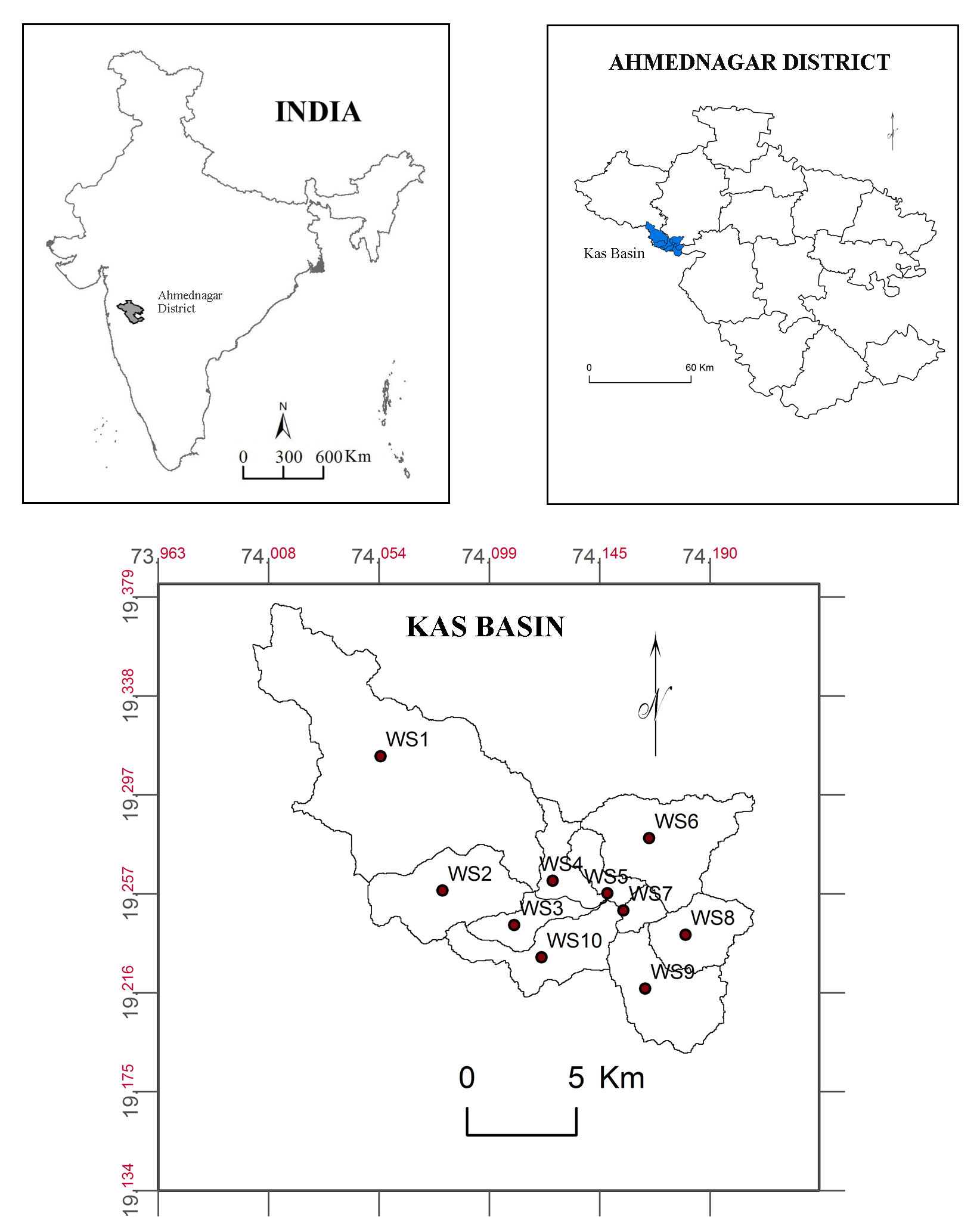
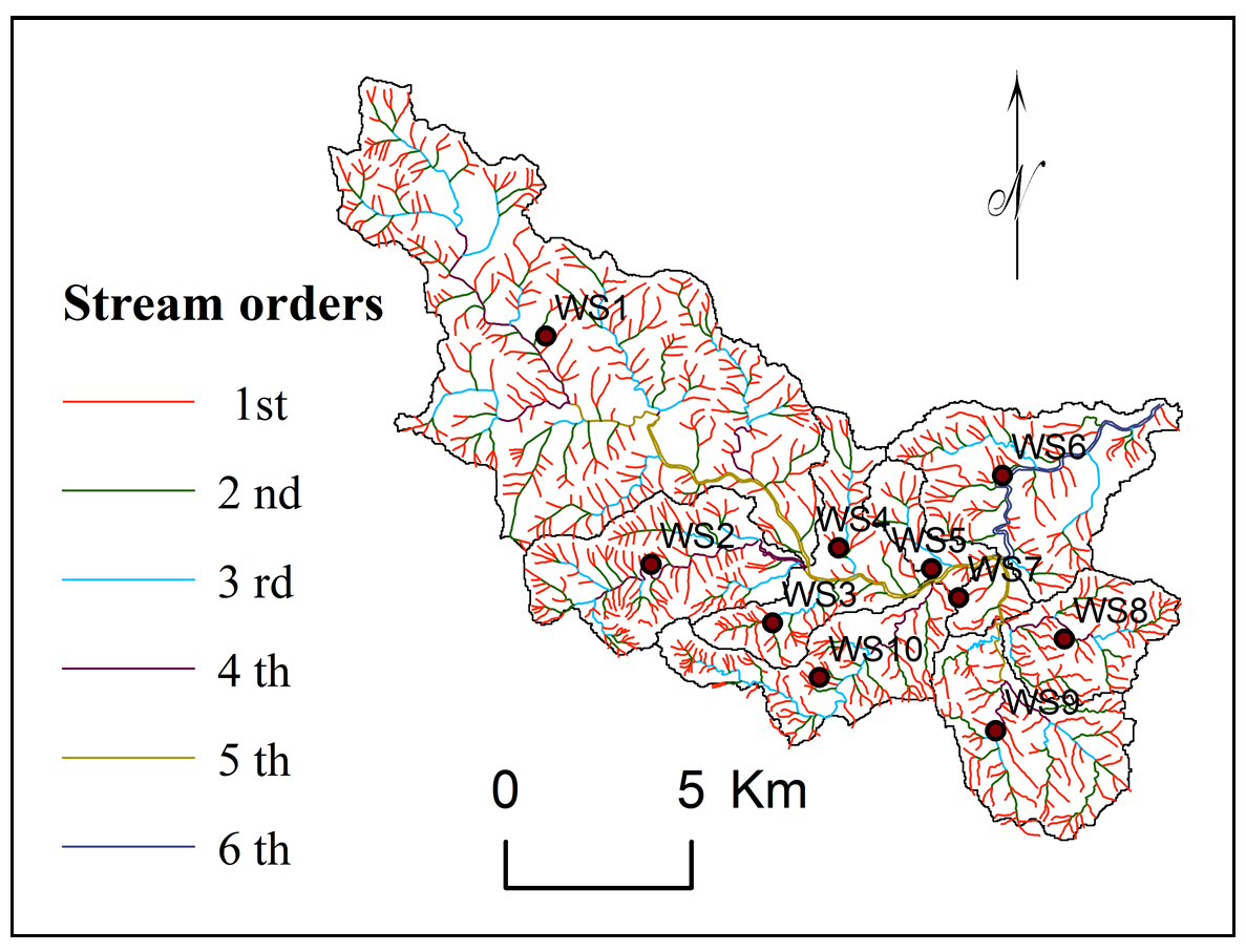
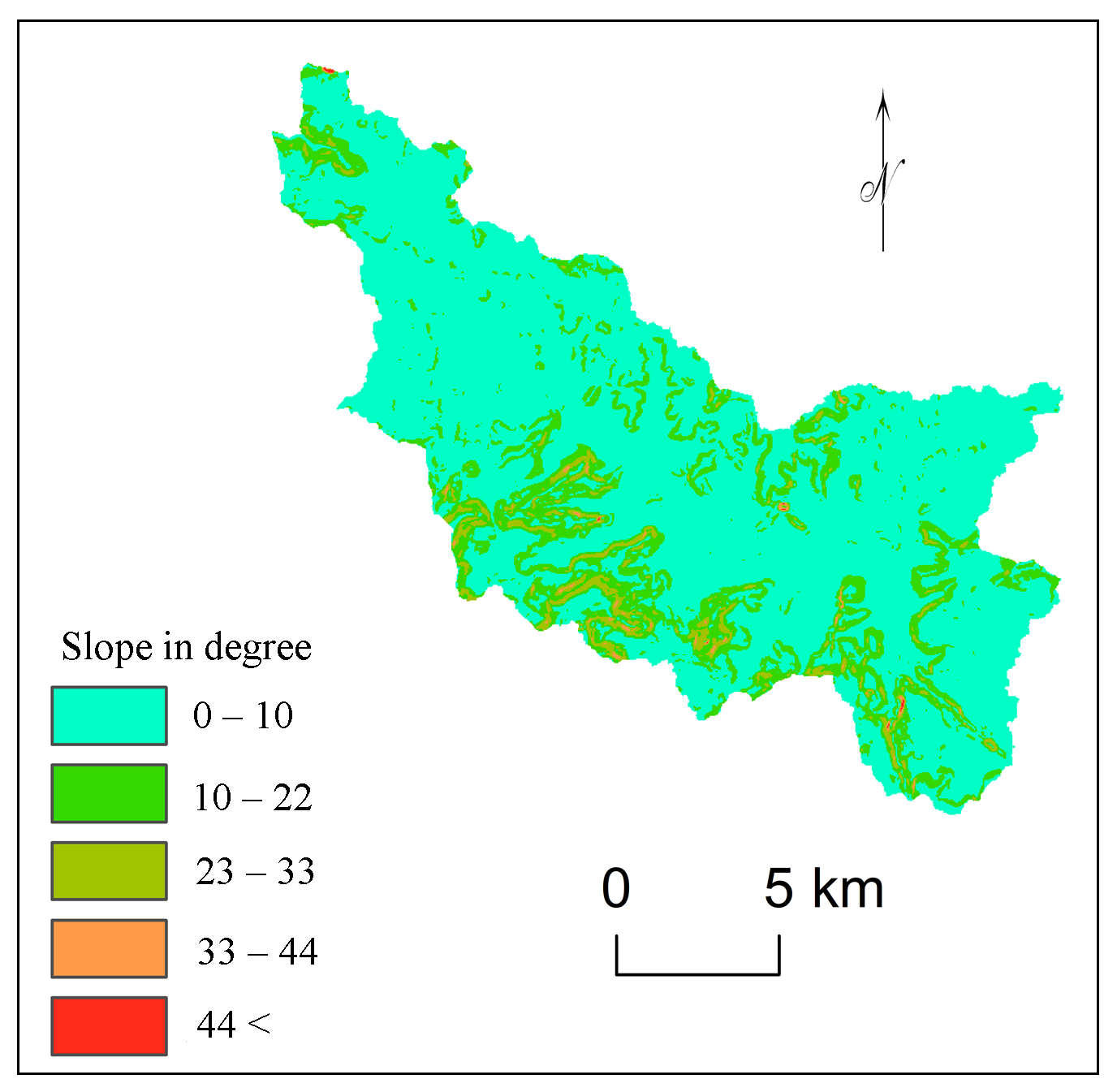
The Kas basin (182.66 sq km) is the part of upper Mula Basin in hilly zone of Deccan plateau in Maharashtra (India) (Figure 1). The region enclosed Aa and pahoehoe basaltic lava flow. The height varies from 620 m to 1060 m. The average annual rainfall is 473 mm, varies from 777 mm at Bramhanwada to 358 mm at Bota. Kas (Figure 2) is tributary of river Mula and receives water from many minor streams. Shallow, very shallow, slightly deep well drained soils are observed with 68.03 % area under crop lands. About 93% basin area observed fine calcareous soil on gently sloping lands with severe and moderate erosion. Cereals like Bajra, Rice and different Pulses, Vegetables, Groundnuts are major crops in the kharip (rainy) season and Jawar, Wheat, Maize and Sunflower are major crops in rabbi (winter) season. Farmers use available surface water and groundwater for seasonal irrigation for vegetables and groundnuts. About 7.42% lands especially on hill slopes (Figure 5) are covered by sparse forests and 16.96% by shrubs and grasses. Majority of population in the region is living below poverty line and facing many problems for livelihood. The Kas basin has been divided into ten sub watershed namely SW1 to SW10 for analysis and prioritization (Zende et al., 2013).
3. Methodology
3.1 Database and Software
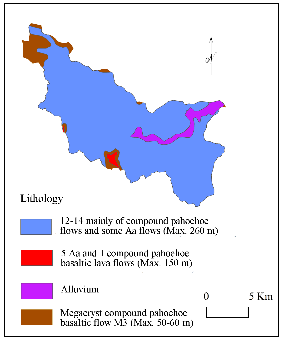
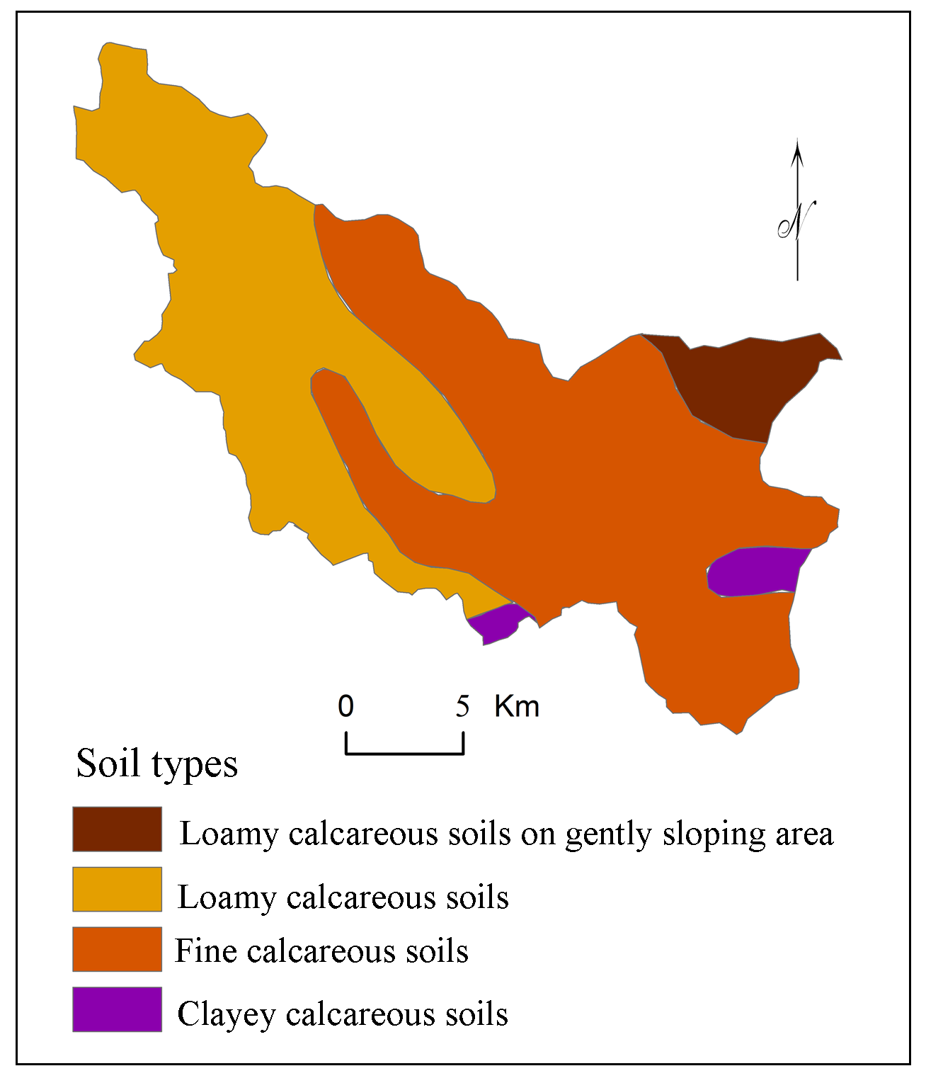
The present analysis (Figure 3) needs information of morphometric parameters, geological and soil characteristics of the region. Maps showing morphometric parameters (Table 1) including linear [Stream Order (\(U\)) , Bifurcation Ratio (\(R_b\)) , Stream Length (\(L_u\)) ], aerial [Basin Area (\(A\)) , Basin Length (\(L_b\)) , Basin Perimeter (\(P\)) , Drainage Density (\(D_d\)) , Stream Frequency (\(F_s\)) , Form Factor (\(R_f\)) , Circularity Ratio (\(R_c\)) , Elongation Ratio (\(R_e\)) , Compactness Coefficient (\(C_C\)) , Drainage Texture (\(D_t\)) ,Texture Ratio (\(T\)) , Drainage Intensity (\(D_i\)) ] and Relief [Relief Ratio (\(R_{h1}\)) , Ruggedness Number (\(R_n\)) ] were prepared from the topographic maps (47I/3 and 47I/4), SOI [survey of India]. ASTER DEM data was used for delineation of watershed boundaries. Geological map (Figure 4) was prepared using map procured from National Institute of Geological Survey, Nagpur (India). Soil map (Figure 6) procured from National Bureau of Soil Survey and Land Use Planning (NBSS and LUP), Government of India for preparation of soil map of Kas basin. Rainfall data was collected from Government of Maharashtra (India) for three rain gauge stations (1992-2013) located within the study area. Topographic, geological and soil map have been loaded and registered (Zeilhofer et al., 2008) in GIS software for preparation of maps.
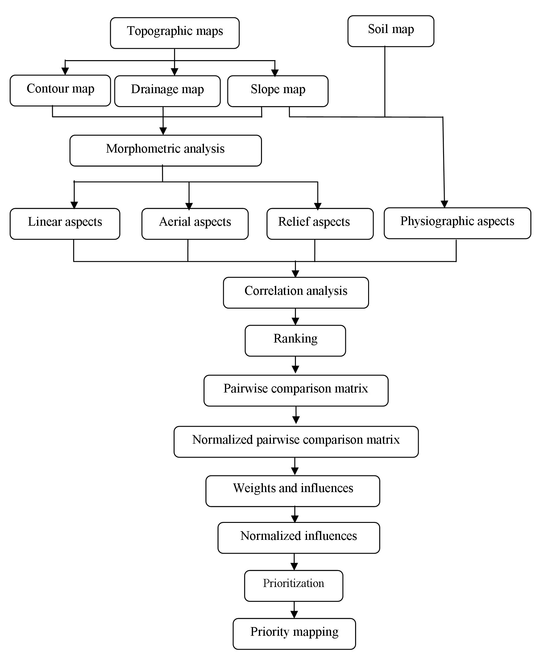
Table 1: Morphometric parameters
|
Aspects |
Parameters |
Equation |
Description |
Author(s) |
|
Linear |
Stream order (\(U\)) |
Hierarchical ranks |
The first step is to determine the stream orders and basin analysis |
|
|
Bifurcation ratio \(R_b\) |
\(R_b = (N_u)/(N_u+1) \) |
\(R_b\) = bifurcation ratio \(N_u\) = number of stream segments |
Kulkarni, 2015; Chitra et al., 2011; Romshoo et al., 2012; Jagadeesh et al., 2014; Aravinda and Balakrishna, 2014; Kedareswarudu, et al., 2013; Iqbal and Sajjad, 2014. |
|
|
Stream length (\(L_u\)) |
\(L_u =\displaystyle\sum_{i=1}^{N} U\) |
\(L_u\) = mean length of channel \(U\) = stream order |
Horton, 1945; Ali et al., 2014; Nongkynrih and Husain, 2011; Kulkarni, 2015. |
|
|
Aerial |
Basin area (\(A\)) |
\(A=a \times n \times10^{-6}\) |
\(a\) : cell area (m2) \(n\) : number of cells in watershed |
|
|
Basin length (\(L_b\)) |
\(L_b\) = farthest distance from watershed ridge to outlet. |
|||
|
Basin perimeter (\(P\)) |
\(P=d \times np \times10^{-3}\) |
\(d\) : cell size (m) \(np\) : number of watershed edge cells |
||
|
Drainage density (\(D_d\)) |
\(D_d =\displaystyle\sum_{}^{} L_u/A\) |
\(D_d\) = drainage density \(L_u\) = total stream length \(A\) = basin area |
Kulkarni, 2015; Nongkynrih and Husain, 2011; Nagal et al., 2014; Aravinda and Balakrishna, 2013; Singh and Singh, 2011. |
|
|
Stream frequency (\(F_s\)) |
\(F_s =\displaystyle\sum_{}^{} N_u/A\) |
\(F_s\) = stream frequency \(N_u\) = number of stream segments \(A\) = basin area |
Kulkarni, 2015; Nongkynrih and Husain, 2011; Nagal et al., 2014; Aravinda and Balakrishna, 2013; Singh and Singh , 2011. |
|
|
Form factor (\(R_f\)) |
\(R_f=A/(L_b+1)^2\) or \(R_f=A/L_a^2\) |
\(R_f\) = form factor \(A\) = basin area \(L_b\) = farthest distance from watershed ridge to outlet or \(A\) = area of the basin \(L_a\) = axial length of the basin. |
Rao and Yusuf, 2013; Ali et al., 2014; Kedareswarudu, et al., 2013; Zende et al., 2013; Nagal et al.,2014; |
|
|
Circularity ratio (\(R_c\)) |
\(R_c=4\pi (A/P^2)\) |
\(R_c\) = circularity ratio \(A\) = basin area (km2) \(P\) = basin perimeter (km) |
Rao and Yusuf, 2013; Iqbal and Sajjad, 2014; Ali et al., 2014. |
|
|
Elongation ratio (\(R_e\)) |
\(R_e = \frac {2}{\pi} \sqrt{\frac {A}{(L_b)^2}} \) or \(R_e = 2 \sqrt{\frac {A}{\pi}/L_u} \) |
\(R_e\) = elongation ratio \( \pi\) =3.14 \(A\) = basin area or \(L_u\) total stream length. |
Aravinda and Balakrishna, 2014; Kedareswarudu, et al., 2013; Khadri and Thakur, 2013; Iqbal and Sajjad, 2014. |
|
|
Compactness coefficient (\(C_C\)) |
\(C_c=0.2821 {\frac {P}{A}}0.5\) |
\(C_C\) = compactness coefficient \(A\) = area of the basin (km²) \(P\) = basin perimeter (km) |
||
|
Drainage texture (\(D_t\)) |
\(D_t=N_u/P\) |
\(N_u\) = total streams of all orders \(P\) =basin perimeter (km) |
||
|
Texture ratio (\(T\)) |
\(T=D_d \times F_s\) |
\(D_d\) drainage density \(F_s\) stream frequency |
||
|
Drainage intensity (\(D_i\)) |
\(D_i=F_s/D_d\) |
\(D_i\) = drainage Intensity \(F_s\) stream frequency \(D_d\) drainage density |
Nagal et al., 2014; Kedareswarudu, et al., 2013; Ali et al., 2014. |
|
|
Relief |
Relief ratio (\(R_{h1}\)) |
\(R_{h1}=B_h/L_b\) |
\(R_{h1}\) = relief ratio \(B_h\) = basin height \(L_b\) = basin length |
|
|
Ruggedness number (\(R_n\)) |
\(R_n=D_d \times (\frac{R}{1000})\) |
\(R_n\) = ruggedness number \(D_d\) = drainage density \(R\) = relief |
3.2 Criterion
Morphometric properties (Zolekar and Bhagat, 2015) have close relationship with watershed planning, management and development. Gharde and Kothari (2016), Gabale and Pawar (2015), Ali and Ali (2014), Rao and Yusuf (2013), Rekha et al. (2011), Romshoo et al. (2012), Singh and Singh, (2011), Sharma et al. (2009), Vandana (2013), Zende et al. (2013), Aravinda and Balakrishna (2013) and Khare et al. (2014) have used the linear, aerial and relief aspects of the prioritization of watershed. Rao et al. (2014), Aouragh and Essahlaoui, (2014), Raja and Karibasappa (2014) and Kiran and Srivastava (2014) have used linear and aerial aspects. Land use/land cover directly reflects the impact of geomorphology, slope, soil, land surface processes, climate, hydrology, etc. as well as human activities (Mishra and Nagarajan, 2010; Panhalkar, 2011; Romshoo et al., 2012; Gashaw et al., 2017). Therefore, Kaur et al. (2014) have used morphometric parameters in combination of land use analysis. Further, Gebre et al. (2015) have added information about changes in land cover and land use, soil type, soil texture with morphometric parameters. Gumma et al. (2014) have used the information of population, slope and rainfall with these parameters for prioritization of watersheds. Vulevic et al. (2015) have used all these parameters for prioritization of watershed using the multi-criteria decision analysis. Here, multi-criteria decision making based on analytical hierarchy process was performed using morphometric parameter and soils. Influences of criterion were calculated using estimated weights and these influence normalized using variations of criterion within selected watersheds. Rainfall is important parameter in prioritization analysis at regional level. However, selected sub-watersheds have no spatial variation in rainfall.
Geology of the region defines nature of subsurface materials, rate of infiltration, amount of runoff, level of ground water and hydraulic conductivity of the surface (Engelhardt et al., 2011; Olden et al., 2012; Dhanalakshmi and Shanmugapriyan, 2015). Bedrock permeability mainly depends on geology and water stability (Flint et al., 2013; Aouragh and Essahlaoui, 2014). Therefore, watershed characteristics are responsive to nature of geology of the region (Gharde and Kothari, 2016). The study area is the part of Deccan trap with 12 to 15 compound pahoehoe flows and some Aa flows (up to 260m), megacryast compound pahoehoe basaltic flows M3 (50 to 60m), 5 Aa and 1 compound pahoehoe basaltic flows M3 (up to 150m) and alluvium type geology (Figure 4). However, no significant spatial variation observed in the region.
3.2.1 Linear Aspects
Khare et al. (2014), Rao et al. (2014), Aouragh and Essahlaoui (2014), Raja and Karibasappa (2014), Kiran and Srivastava (2014) and Farhan and Anaba (2016) have used linear parameters: stream order (\(U\)), stream length (\(L_u\)), mean stream length (\(L_{sm}\)) , (Wilson et al., 2012), stream length ratio, bifurcation ratio (\(R_b\)) . These parameters are related with land surface erodibility. Therefore, linear aspects of the study area: stream order (\(U\)) , stream number (\(N_u\)) , bifurcation ratio (\(R_b\)) , mean stream length (\(L_{sm}\)) and stream length (\(L_u\)) , are selected for analysis of selected watersheds for prioritization.
a. Stream Order (\(U\))
Stream orders indicate lithology, physiography, structure and uniformity of rocks in the watershed (Singh and Singh, 2011; Vandana, 2013; Chitra et al., 2011; Zende et al., 2013; Ali and Ali, 2014). Streams are appeared as the segments in GIS. The orders of these segments are calculated with the help of GIS software, Global Maper 11. About 79% streams (809) are recognized as first order (Table 2), 16.11% (165) second order, 3.52% (36) third order, 0.78% (08), fourth order and 0.49 (05) fifth order. The sub-watersheds: WS1, WS2, WS3, WS4 and WS5 were delineated at fifth order of streams.
Table 2. Stream orders and bifurcation ratio
|
Sub-watersheds |
Stream orders |
Bifurcation ratios |
|||||||||||
|
Ist |
IInd |
IIIrd |
IVth |
Vth |
VIth |
\(R_b1\) |
\(R_b2\) |
\(R_b3\) |
\(R_b4\) |
\(R_b5\) |
Total |
Mean |
|
|
WS1 |
309 |
64 |
12 |
4 |
1 |
0 |
5.83 |
6.33 |
4.00 |
5.00 |
0.00 |
21.16 |
4.23 |
|
WS2 |
120 |
28 |
7 |
1 |
0 |
0 |
5.29 |
5.00 |
8.00 |
0.00 |
0.00 |
18.29 |
3.66 |
|
WS3 |
32 |
7 |
1 |
0 |
0 |
0 |
4.57 |
7 |
0 |
0 |
0 |
11.57 |
2.89 |
|
WS4 |
24 |
7 |
1 |
0 |
0 |
0 |
3.42 |
7 |
0 |
0 |
0 |
10.43 |
2.61 |
|
WS5 |
18 |
4 |
1 |
0 |
1 |
0 |
5.50 |
5.00 |
0.00 |
1.00 |
0.00 |
11.50 |
2.30 |
|
WS6 |
90 |
22 |
4 |
0 |
0 |
1 |
5.09 |
6.50 |
0.00 |
0.00 |
1.00 |
12.59 |
2.52 |
|
WS7 |
10 |
2 |
0 |
0 |
1 |
0 |
6.00 |
0.00 |
0.00 |
1.00 |
0.00 |
7.00 |
1.40 |
|
WS8 |
58 |
10 |
4 |
1 |
0 |
0 |
6.80 |
3.50 |
5.00 |
0.00 |
0.00 |
15.30 |
3.06 |
|
WS9 |
75 |
14 |
5 |
2 |
1 |
0 |
6.36 |
3.80 |
3.50 |
3.00 |
0.00 |
16.66 |
3.33 |
|
WS10 |
81 |
19 |
2 |
1 |
0 |
0 |
5.26 |
10.50 |
3.00 |
0.00 |
0.00 |
18.76 |
3.75 |
b. Bifurcation Ratio (\(R_b\))
Bifurcation ratio indicates the shape of basin, branching pattern, surface erodibility. Higher \(R_b\) values show an elongated basin whereas lesser represents circular basin (Chitra et al., 2011; Khare et al., 2014). It is the ratio between the total number of first order streams to that of the next higher order streams in the basin (Pareta and Pareta, 2011; Iqbal and Sajjad, 2014). The lesser values indicate less structural disturbances (Strahler, 1964) with stable drainage (Pareta and Pareta, 2011) (Table 2) whereas more values indicate a strong structural control over drainage system (Chitra et al., 2011). The bifurcation ratio varies from 2.97 to 6.74 and indicates higher erosion activity in the basin (Strahler, 1957; Rai at el., 2014) and need of soil conservation.
c. Stream Length (\(L_u\))
Stream length indicates surface run-off characteristics like slopes steepness, lithology and topography (Nongkynrih and Husain, 2011; Chitra et al., 2011; Iqbal and Sajjad, 2014). The stream length of each order of stream in Kas basin has been measured from topographic maps (Nagal, et al., 2014). Longer streams have permeable bedrock and well-drained network (Kulkarni, 2015). Stream number and length are observed higher for first order and decreases according to increasing stream order. Total length of first order streams is estimated about 395.78 km (62.61%), second order streams 116.81 km (18.48%), third order streams 66.11 km (10.46%), fourth order streams 28.47 km (4.50%), fifth order streams 16.3 km. (2.58%) and sixth order streams 8.71 km (1.38%) (Table 3).
Table 3: Stream length
|
Watersheds |
Stream orders |
|||||
|
Ist (km) |
IInd (km) |
IIIrd (km) |
IVth (km) |
Vth (km) |
VIth (km) |
|
|
WS1 |
149.66 |
46.59 |
26.5 |
11.28 |
6.82 |
0 |
|
WS2 |
50.07 |
12.55 |
9.1 |
7.45 |
0 |
0 |
|
WS3 |
13.8 |
5 |
2.05 |
0 |
0 |
0 |
|
WS4 |
13.24 |
4.45 |
3.14 |
0 |
0 |
0 |
|
WS5 |
7.81 |
1.56 |
2.3 |
0 |
1.75 |
0 |
|
WS6 |
46.88 |
12.73 |
7.14 |
0 |
0 |
8.71 |
|
WS7 |
5.62 |
1.39 |
0 |
0 |
1.93 |
0 |
|
WS8 |
29.3 |
8.01 |
2.66 |
3.04 |
0 |
0 |
|
WS9 |
41.24 |
14.05 |
5.05 |
3.55 |
1.98 |
0 |
|
WS10 |
38.33 |
10.48 |
8.18 |
3.15 |
0 |
0 |
|
Total |
395.95 |
116.81 |
66.12 |
28.47 |
12.48 |
8.71 |
3.2.2 Aerial Aspects
Aerial aspects including basin area, basin length, basin perimeter, drainage density, stream frequency, form factor, circularity ratio, elongation ratio, compactness coefficient, drainage texture, texture ratio, drainage intensity and infiltration number are selected for the analysis.
a. Basin Area (\(A\))
Basin area is indicator of size (Strahler, 1957) and significant for calculating the drainage density (\(D_d\)) , stream frequency (\(F_s\)) , form factor (\(R_f\)) , circularity ratio (\(R_c\)) , elongation ratio (\(R_e\)) , compactness coefficient (\(C_C\)) and lemniscates (\(k\)) (Gabale and Pawar, 2015; Kothari and Garde, 2016). The Kas River drains over 181.65 km2 (Figure 2) (Table 4).
Table 4. Parameters
|
Sub- Watershed |
Parameters |
|||||||||||||||||||
|
\(R_b\) |
\(L_u\) |
\(A\) |
\(L_b\) |
\(P\) |
\(D_d\) |
\(F_s\) |
\(R_f\) |
\(R_c\) |
\(R_e\) |
\(C_C\) |
\(D_t\) |
\(T\) |
\(D_i\) |
\(I_f\) |
\(R_{h1}\) |
\(R_n\) |
Slope |
Soil |
||
|
WS1 |
4.23 |
231.86 |
75.9 |
15.42 |
69.82 |
3.05 |
5.05 |
0.32 |
0.20 |
0.64 |
2.26 |
5.49 |
5.49 |
1.65 |
15.41 |
0.07 |
3.30 |
41.32 |
64.58 |
|
|
WS2 |
3.66 |
76.78 |
18.96 |
7.07 |
27.61 |
4.05 |
8.23 |
0.38 |
0.31 |
0.70 |
1.79 |
5.65 |
5.65 |
2.03 |
33.32 |
0.15 |
4.29 |
11.47 |
13.79 |
|
|
WS3 |
2.89 |
20.68 |
6.48 |
4.10 |
18.94 |
18.94 |
6.17 |
0.39 |
0.23 |
0.70 |
2.10 |
2.11 |
2.11 |
1.65 |
116.91 |
32.93 |
7.13 |
3.02 |
2.80 |
|
|
WS4 |
2.61 |
20.04 |
7.23 |
5.41 |
21.05 |
21.05 |
4.15 |
0.25 |
0.20 |
0.56 |
2.21 |
1.43 |
1.43 |
2.03 |
87.34 |
23.66 |
6.08 |
3.30 |
0.00 |
|
|
WS5 |
2.30 |
14.05 |
4.93 |
7.05 |
17.97 |
2.85 |
4.67 |
0.10 |
0.19 |
0.36 |
2.28 |
1.28 |
1.28 |
1.64 |
13.30 |
0.11 |
2.28 |
2.56 |
0.00 |
|
|
WS6 |
2.52 |
74.80 |
22.76 |
7.45 |
32.2 |
3.29 |
5.01 |
0.41 |
0.28 |
0.72 |
1.90 |
3.54 |
3.54 |
1.52 |
16.46 |
0.11 |
2.69 |
10.56 |
0.00 |
|
|
WS7 |
1.40 |
8.88 |
2.82 |
2.25 |
9.95 |
3.15 |
4.61 |
0.56 |
0.36 |
0.84 |
1.67 |
1.31 |
1.31 |
1.46 |
14.52 |
0.34 |
2.39 |
1.77 |
1.24 |
|
|
WS8 |
3.03 |
42.39 |
10.82 |
4.36 |
18.63 |
3.92 |
6.47 |
0.57 |
0.39 |
0.85 |
1.60 |
3.76 |
3.76 |
1.65 |
25.35 |
0.21 |
3.60 |
6.78 |
0.00 |
|
|
WS9 |
3.33 |
64.63 |
17.44 |
6.2 |
26.05 |
3.71 |
5.50 |
0.45 |
0.32 |
0.76 |
1.76 |
3.69 |
3.69 |
1.49 |
20.40 |
0.15 |
3.41 |
10.92 |
5.31 |
|
|
WS10 |
3.75 |
60.22 |
14.42 |
8.45 |
30.27 |
4.18 |
6.93 |
0.20 |
0.20 |
0.51 |
2.25 |
3.30 |
3.30 |
1.66 |
28.96 |
0.12 |
4.34 |
8 |
12.27 |
|
b. Basin Length (\(L_b\))
Basin length indicates basin shape and hydrological characteristics (Chitra et al., 2011) including lemniscate’s value, form factor and elongation ratio (Pareta and Pareta, 2011; Nagal et al., 2014). The basin length in the study area varies from 15 km (WS1) to 2.25 km (WS6) (Table 4). Maximum basin length indicates more texture, infiltration number and basin perimeter showing need of conservation.
c. Basin Perimeter (\(P\))
Basin perimeter is the length of outer boundary of the watershed forms the size, shape and drainage density (Strahler, 1957; Nagal et al., 2014). The perimeter of Kas basin is 85.19 km and varies for sub-watersheds from 69.82 km for WS1 to 9.95 km for WS4.
d. Drainage Density (\(D_d\))
Drainage density is useful for analysis of terrain, rocks, relief, soils, groundwater, erodibility and discharge of water and sediment (Pareta and Pareta, 2011; Engelhardt et al., 2011; Kaur et al., 2014; Gebre et al., 2015; Gabale and Pawar, 2015). Drainage densities in this watershed can be categorized (Gebre et al., 2015) as very coarse (2.17 to 3.92 km/km2) and moderate (3.29 to 4.18 km/km2) (Table 4). Higher values of \(D_d\) indicates moderate slopes (Vandana, 2013; Argyriou et al., 2016) with semi-permeable hard rock, coarse textures, favorable conditions for groundwater conservation (Khare et al., 2014; Gebre et al., 2015; Gabale and Pawar, 2015). Drainage densities in Kas basin vary from 2.85 to 4.18 km/km2 (Table 4).
e. Stream Frequency (\(F_s\))
Stream frequency indicates nature of subsurface materials, relief, infiltration rate, permeability, stream population, vegetative cover and have relationship with drainage density (Chatterjee and Tantubay, 2000; Pareta and Pareta, 2011; Singh and Singh, 2011; Chitra et al., 2011; Romshoo et al., 2012; Vandana, 2013; Patel et al., 2013; Iqbal and Sajjad, 2014; Rai et al., 2014; Kaur et al., 2014; Gebre et al.,2015; Farhan and Al-Shaikh, 2017). Stream frequency depends on lithology, rock structure, subsurface permeability, infiltration capacity, relief, drainage network, rainfall, vegetation cover, etc. (Wilson et al., 2012; Aouragh and Essahlaoui, 2014; Gabale and Pawar, 2015; Kulkarni, 2015; Raja and Karibasappa, 2016; Argyriou et al., 2016). Sub-watersheds with dense forest show less frequency of streams in drainage network whereas agricultural lands show higher frequency (Zende et al., 2013). Stream frequency in the region varies from 2.31 to 6.47 km/km2 (Table 4). Higher stream frequencies of WS2 (8.23), WS7 (6.47) and WS9 (6.93) indicate impermeability and less infiltration capacity of subsurface and higher relief with thin vegetation cover.
f. Form Factor (\(R_f\))
The form factor, \(R_f\) indicates shape (Rai et al., 2014) and length of basin (Patel et al., 2013). The elongated watershed estimates less value and nearly circular watersheds show higher values (Gabale and Pawar, 2015). Perfectly circular watershed shows form factor about 0.75 (Pareta and Pareta, 2011). WS6 (0.56), WS7 (0.57) and WS8 (0.45) (Table 4) are nearly circular whereas WS1 (0.32), WS2 (0.38) and WS3 (0.35) are moderate elongated and WS4 (0.10) and WS9 (0.20) are more elongated.
g. Circularity Ratio (\(R_c\))
Circularity ratio indicates flow of discharge, erosion, (Patel et al., 2013; Rao and Yusuf, 2013), stage of topography and shapes (Gray, 1961; Ali and Ali, 2014; Farhan and Anaba, 2016). Length and frequency of tributaries, geological structures, land use/land cover, climate, relief and slope of the basin affect the circularity ratio (Mishra and Nagarajan, 2010; Nongkynrih and Husain, 2011; Chitra et al., 2011; Iqbal et al., 2013; Kaur et al., 2014; Farhan and Anaba, 2016). Estimated circularity ratios (0.16 to 0.39) for watersheds in the region indicate high erosion with permeable homogeneous geology (Aravinda and Balakrishna, 2014; Wilson et al., 2012; Farhan and Anaba, 2016). Less circularity ratios for WS1 (0.20), WS3 (0.16), WS4 (0.19 and WS9 (0.20) indicate dendritic stage, whereas WS2 (0.31), WS5 (0.28), WS6 (0.36), WS7 (0.39) and WS8 (0.32) are comparatively mature dendritic streams (Table 4).
h. Elongation Ratio (\(R_e\))
Elongation ratio indicates shape, hydrology, slope, infiltration and runoff (Kaur et al., 2014; Iqbal and Sajjad, 2014; Zende et al., 2013; Wilson et al., 2012; Chitra et al., 2011; Mishra and Nagarajan, 2010). Elongation ratio is the ratio between the diameter and the maximum length of the basin (Nongkynrih and Husain, 2011; Strahler, 1964). Higher elongation ratios show more infiltration capacity of land surface and less runoff (Iqbal and Sajjad, 2014). WS6 (0.84) and WS7 (0.85) show oval shapes with more infiltration capacity of land surface; WS2 (0.70), WS5 (0.72) and WS8 (0.76) show less infiltration capacity and more runoff, whereas WS1 (0.64), WS3 (0.67), WS4 (0.36) and WS9 (0.51) show nearly elongated shape with less runoff and more infiltration. Therefore, watershed with higher relief and steep slopes should be selected for conservation purpose with high priority (Table 4).
i. Compactness Coefficient (\(C_C\))
Compactness coefficient indicates erosion risk and relationship of hydrology of the basin (Ali et al., 2014; Iqbal et al., 2013). Nagal et al. (2014) and Patel et al. (2013) have described the compactness coefficient dependent on size and slope in the watersheds. Estimated compactness coefficients in the study area vary from 1.60 to 2.48. WS1 (2.26), WS3 (2.48), WS4 (2.28) and WS9 (2.25) show high compactness coefficient which indicate less elongation and high erosion whereas WS2 (1.79), WS5 (1.90), WS6 (1.67), WS7 (1.60) and WS8 (1.76) show more elongation and less erosion (Table 4).
j. Drainage Texture (\(D_t\))
Drainage texture indicates lithology of the watershed (Rao and Yusuf, 2013). Drainage texture shows influence of climate, vegetation, rock, soil, infiltration capacity, relief, etc. (Kulkarni, 2015; Aouragh and Essahlaoui, 2014; Vandana, 2013; Iqbal et al., 2013; Chatterjee and Tantubay, 2000). Smith (1950) has been classified drainage density into five categories of drainage texture. The watersheds in the study area: WS3, WS4, WS5, WS6, WS7, WS8 and WS9 show coarse drainage texture (1.28 to 5.65). WS1 (5.49) and WS2 (5.65) indicate intermediate texture (Table 4) which are favorable for resource conservation.
k. Texture Ratio (\(T\))
Texture ratio indicates morphometric structure, runoff and drainage texture of the basin (Farhan and Anaba, 2016; Nagal et al., 2014). It depends on lithology, infiltration capacity and relief in the region (Farhan and Anaba, 2016, Khare et al., 2014; Rekha et al., 2011; Pareta and Pareta, 2011). WS1 (5.49) and WS2 (5.65) show higher texture ratio with high relief and intermediate topography; WS4 (1.28) and WS6 (1.31) show very coarse texture and WS3 (2.13), WS5 (3.54), WS7 (3.76), WS8 (3.69) and WS9 (3.30) show course topography and moderate runoff. Estimated ratio values are classified into four categories after Smith (1950).
l. Drainage Intensity (\(D_i\))
Drainage intensity indicates runoff, flooding, gully erosion, landslides and denudation of the basin (Gabale and Pawar, 2015; Pareta and Pareta, 2011). The drainage intensity is the ratio between stream frequency and drainage density (Nagal et al., 2014). Drainage intensity in the study area varies from 1.46 to 2.03 (Table 5). Watersheds in the region indicate small influence of drainage density and stream frequency.
Table 5. Correlation matrix
|
\(R_b\) |
\(L_u\) |
\(A\) |
\(L_b\) |
\(P\) |
\(D_d\) |
\(F_s\) |
\(R_f\) |
\(R_c\) |
\(R_e\) |
\(C_C\) |
\(D_t\) |
\(T\) |
\(D_i\) |
\(I_f\) |
\(R_{h1}\) |
\(R_n\) |
Slope |
Soil |
|
|
\(R_b\) |
1 |
||||||||||||||||||
|
\(L_u\) |
0.73 |
1 |
|||||||||||||||||
|
\(A\) |
0.67 |
0.99 |
1 |
||||||||||||||||
|
\(L_b\) |
0.74 |
0.92 |
0.92 |
1 |
|||||||||||||||
|
\(P\) |
0.74 |
0.98 |
0.98 |
0.96 |
1 |
||||||||||||||
|
\(D_d\) |
-0.12 |
-0.34 |
-0.29 |
-0.3 |
-0.24 |
1 |
|||||||||||||
|
\(F_s\) |
0.55 |
0.07 |
-0.03 |
0.01 |
0.01 |
-0.19 |
1 |
||||||||||||
|
\(R_f\) |
-0.22 |
-0.05 |
-0.06 |
-0.42 |
-0.2 |
-0.15 |
0.13 |
1 |
|||||||||||
|
\(R_c\) |
-0.28 |
-0.22 |
-0.26 |
-0.53 |
-0.39 |
-0.36 |
0.25 |
0.9 |
1 |
||||||||||
|
\(R_e\) |
-0.13 |
0.02 |
0 |
-0.36 |
-0.12 |
-0.12 |
0.18 |
0.99 |
0.86 |
1 |
|||||||||
|
\(C_C\) |
0.28 |
0.24 |
0.28 |
0.55 |
0.41 |
0.33 |
-0.26 |
-0.9 |
-0.99 |
-0.87 |
1 |
||||||||
|
\(D_t\) |
0.81 |
0.77 |
0.7 |
0.63 |
0.69 |
-0.43 |
0.61 |
0.19 |
0.16 |
0.26 |
-0.17 |
1 |
|||||||
|
\(T\) |
0.81 |
0.77 |
0.7 |
0.63 |
0.69 |
-0.43 |
0.61 |
0.19 |
0.16 |
0.26 |
-0.17 |
1 |
1 |
||||||
|
\(D_i\) |
0.3 |
-0.01 |
-0.03 |
0.07 |
0.03 |
0.48 |
0.32 |
-0.34 |
-0.28 |
-0.29 |
0.25 |
0.18 |
0.18 |
1 |
|||||
|
\(I_f\) |
-0.03 |
-0.33 |
-0.3 |
-0.32 |
-0.25 |
0.96 |
0.03 |
-0.09 |
-0.31 |
-0.05 |
0.27 |
-0.33 |
-0.33 |
0.43 |
1 |
||||
|
\(R_{h1}\) |
-0.13 |
-0.33 |
-0.28 |
-0.31 |
-0.24 |
0.97 |
-0.15 |
-0.1 |
-0.35 |
-0.07 |
0.31 |
-0.43 |
-0.43 |
0.34 |
0.98 |
1 |
|||
|
\(R_n\) |
0.22 |
-0.19 |
-0.18 |
-0.18 |
-0.11 |
0.89 |
0.23 |
-0.11 |
-0.32 |
-0.04 |
0.28 |
-0.11 |
-0.11 |
0.53 |
0.96 |
0.9 |
1 |
||
|
Slope |
0.7 |
1 |
1 |
0.91 |
0.97 |
-0.32 |
0.01 |
-0.04 |
-0.22 |
0.02 |
0.25 |
0.73 |
0.73 |
-0.03 |
-0.32 |
-0.31 |
-0.19 |
1 |
|
|
Soil |
0.68 |
0.95 |
0.95 |
0.89 |
0.94 |
-0.24 |
0.04 |
-0.14 |
-0.33 |
-0.08 |
0.36 |
0.64 |
0.64 |
0.04 |
-0.23 |
-0.22 |
-0.1 |
0.96 |
1 |
m. Infiltration Number (\(I_f\))
Infiltration number indicates infiltration characteristics, runoff, vegetation cover and permeability of soil cover (Nagal et al., 2014; Rao and Yusuf, 2013; Ranjan, 2013; Singh and Singh, 2011). Normally infiltration number of any watershed is defined as the product of drainage density and stream frequency (Nagal et al., 2014). Infiltration numbers vary from 13.30 to 33.32. WS1 (15.41), WS3 (16.79), WS5 (16.46) and WS6 (14.52) show more runoff during rain spells.
3.2.3 Relief Aspects
a. Relief Ratio (\(R_{h1}\))
Relief ratio is important to understand overall slope, relief and erosion process in the watershed (Strahler, 1957; Chatterjee and Tantubay, 2000; Sharma et al., 2009; Engelhardt et al., 2011; Wilson et al., 2012; Vandana, 2013; Kaur et al., 2014; Yunus et al., 2014). The relief ratio is defined as the ratio between the total relief of a basin and the longest dimension of the basin similar to the main drainage line (Nagal et al., 2014). Relief ratios in the region vary from 0.07 to 0.34 (Table 4). The relief ratio normally increases with decreasing drainage area and size of the basin. Relief ratios for WS1, WS2, WS3, WS4, WS5, WS8 and WS9 indicate moderate slopes whereas WS6 (0.21) and WS7 (0.34) show high relief ratio.
b. Ruggedness Number (\(R_n\))
Ruggedness values indicate nature of relief, drainage density, slope, soil erosion, topography, lithology and discharge through the streams (Chitra et al., 2011; Pareta and Pareta, 2011; Rao et al., 2004; Nagal et al., 2014; Aouragh and Essahlaoui, 2014). The ruggedness number is the product of basin relief and drainage density. It is usefully relationship with steepness and length to understand the relief and drainage density (Kaur et al., 2014; Nagal et al., 2014). Higher \(R_n\) indicates irregular topography, lithological heterogeneity, high drainage density and high soil erosion. \(R_n\) values for WS4, WS5 and WS6 are moderate indicating flat surface, moderate degree of dissection and soil erosion.
3.2.4 Physiographic Aspects
a. Slope
Slope analysis is helpful to identify the potential sites for watershed management (Zolekar and Bhagat, 2015; Argyriou et al., 2016). Slope is significantly affecting the morphometric aspects and drainage characteristics in the region (Kothari and Garde, 2016; Patel et al., 2013). Slope plays key role in formation of amount of runoff, rate of infiltration (Sepehr et al., 2017), drainage density (Nagal et al., 2014; Kaur et al., 2014; Argyriou et al., 2016; Rekha et al., 2011; Wilson et al., 2012), intensity of flood, quantity of erosion (Chang et al., 2013), soil depth, etc. The gentle slope shows less potentials of construction for water storages (Emamgholi et al., 2007). Land with moderate slope (10º-22º) is more suitable for conservation of resources and key criterion in watershed management. Therefore, area with moderate slopes was considered as the criterion for analysis of sub-watershed prioritization in the study area.
b. Soil
Soil is vital natural resources supporting life systems and socio-economic development (Ranjan, 2013). Soil erosion is a major problem in rain-fed area. Erosion of the top soil layer leads to constant land degradation and decline of soil quality and productivity (Farhan and Anaba, 2016; Yeole et al., 2012). Soil characteristics (Capodici et al., 2013) like texture, structure, organic matter content and permeability are useful to interpret the soil erodibility (Shinde et al., 2010). Soil map for Kas basin is prepared from map procured from National Bureau of Soil Survey and Land Use Planning (NBSS and LUP), Government of India. Clayey, loamy, calcareous, fine-loamy and fine calcareous soils are observed in the study area (Figure 6).
3.3 Analytical Hierarchy Process (AHP) for Watershed Prioritization
Prioritization of sub-watersheds was processed using AHP in six steps: (1) determination of rank, (2) pairwise comparison matrix, (3) preparation of normalized pairwise comparison matrix, (4) calculation of weights and influence, (5) normalization of influence and (6) prioritization of watersheds.
3.3.1 Determination Rank
Quantitative and qualitative methods have been widely used for determination of ranks to the parameters selected for weighted analyses. Scholars likes Sepehr et al., (2017), Ghanbarpour and Hipel, (2011), Rekha et al., (2011), Feizizadeh el al., (2014), etc. have used multi-criteria decision-making and pair wise comparison matrix. Zolekar and Bhagat (2015) have used expert opinions and correlation techniques for ranking the parameters in AHP based weighted overlay analysis for land suitability analyses. Bhagat (2012) has expressed that the correlation analysis is useful for better understanding of unstandardized parameters than the standardized parameters. Here, ranks of selected criterion have been determined based on sum of significant correlation coefficients estimated within the groups of criterions (Table 5).
Correlation between different 19 physiographic and morphometric parameters (Table 4) estimated using Pearson’s correlation technique (Yin et al., 2012) (Table 5). Yunus et al. (2014) and Farhan and Al-Shaikh (2017) have classified significant correlation values into three categories: strong correlation (0.8 to 0.9), good (0.7 to 0.8), moderate (0.5 to 0.7) and less than 0.5 insignificant (Table 5). Criterion selected for this study assigned ranks from 1 to 19 based on sum of the calculated significant positive correlations within the groups (Ranjan, 2013; Zolekar and Bhagat, 2015; Farhan and Anaba, 2016; Argyriou et al., 2016). Drainage Texture (\(D_t\)) , Texture Ratio (\(T\)), Bifurcation Ratio (\(R_b\)) , Geology and Stream Length (\(L_u\)) show more influence on erosion in hilly and foothill zones, therefore they are ranked 1 to 5, respectively. The criterion like Slope, Basin Area, Basin Perimeter, Ruggedness Number and Stream Frequency show moderate influence on surface erosion. They are ranked from 6 to 10 and further, Infiltration Number, Basin Length, Drainage Density, Drainage Intensity, Soil, Elongation Ratio, Form Factor, Compactness Coefficient and Relief Ratio were assigned ranks according to sum of significance values (Table 6).
Table 6. Ranking
|
Criterion |
\(L_u\) |
\(D_t\) |
\(T\) |
\(P\) |
Slope |
\(R_b\) |
\(L_b\) |
\(A\) |
Soil |
\(R_n\) |
\(C_C\) |
\(D_d\) |
\(I_f\) |
\(R_{h1}\) |
\(D_i\) |
\(F_s\) |
\(R_e\) |
\(R_f\) |
\(R_c\) |
|
Ranks |
1 |
2 |
3 |
4 |
5 |
6 |
7 |
8 |
9 |
10 |
11 |
12 |
13 |
14 |
15 |
16 |
17 |
18 |
19 |
3.3.2 Pairwise Comparison Matrix (PCM)
Pairwise comparison matrix has been performed (Table 7) to calculate the weights for calculation of influence of criterion (Zolekar and Bhagat, 2015) on the surface erosion (Elaalem, 2012). The PCM helps to understand the relationship between the criterion in relation to surface erosion and influence in assessment for applications of conservation techniques in the watershed (Emamgholi et al., 2007; Ranjan, 2013). The criterion values in PCM were divided by total of the column to find the cell values in normalized pairwise comparison matrix (Table 8).
Table 7. Pairwise comparison matrix
|
Criterion |
\(L_u\) |
\(D_t\) |
\(T\) |
\(P\) |
Slope |
\(R_b\) |
\(L_b\) |
\(A\) |
Soil |
\(R_n\) |
\(C_C\) |
\(D_d\) |
\(I_f\) |
\(R_{h1}\) |
\(D_i\) |
\(F_s\) |
\(R_e\) |
\(R_f\) |
\(R_c\) |
|
\(L_u\) |
1/1 |
2/2 |
3/3 |
4/4 |
5/5 |
6/6 |
7/7 |
8/8 |
9/9 |
10/10 |
11/11 |
12/12 |
13/13 |
14/14 |
15/15 |
16/16 |
17/17 |
18/18 |
19/19 |
|
\(D_t\) |
2/2 |
3/2 |
4/2 |
5/2 |
6/2 |
7/2 |
8/2 |
9/2 |
10/2 |
11/2 |
12/2 |
13/2 |
14/2 |
15/2 |
16/2 |
17/2 |
18/2 |
19/2 |
|
|
\(T\) |
3/3 |
4/3 |
5/3 |
6/3 |
7/3 |
8/3 |
9/3 |
10/3 |
11/3 |
12/3 |
13/3 |
14/3 |
15/3 |
16/3 |
17/3 |
18/3 |
19/3 |
||
|
\(P\) |
4/4 |
5/4 |
6/4 |
7/4 |
8/4 |
9/4 |
10/4 |
11/4 |
12/4 |
13/4 |
14/4 |
15/4 |
16/4 |
17/4 |
18/4 |
19/4 |
|||
|
Slope |
5/5 |
6/5 |
7/5 |
8/5 |
9/5 |
10/5 |
11/5 |
12/5 |
13/5 |
14/5 |
15/5 |
16/5 |
17/5 |
18/5 |
19/5 |
||||
|
\(R_b\) |
6/6 |
7/6 |
8/6 |
9/6 |
10/6 |
11/6 |
12/6 |
13/6 |
14/6 |
15/6 |
16/6 |
17/6 |
18/6 |
19/6 |
|||||
|
\(L_b\) |
7/7 |
8/7 |
9/7 |
10/7 |
11/7 |
12/7 |
13/7 |
14/7 |
15/7 |
16/7 |
17/7 |
18/7 |
19/7 |
||||||
|
\(A\) |
8/8 |
9/8 |
10/8 |
11/8 |
12/8 |
13/8 |
14/8 |
15/8 |
16/8 |
17/8 |
18/8 |
19/8 |
|||||||
|
Soil |
9/9 |
10/9 |
11/9 |
12/9 |
13/9 |
14/9 |
15/9 |
16/9 |
17/9 |
18/9 |
19/9 |
||||||||
|
\(R_n\) |
10/10 |
11/10 |
12/10 |
13/10 |
14/10 |
15/10 |
16/10 |
17/10 |
18/10 |
19/10 |
|||||||||
|
\(C_C\) |
11/11 |
12/11 |
13/11 |
14/11 |
15/11 |
16/11 |
17/11 |
18/11 |
19/11 |
||||||||||
|
\(D_d\) |
12/12 |
13/12 |
14/12 |
15/12 |
16/12 |
17/12 |
18/12 |
19/12 |
|||||||||||
|
\(I_f\) |
13/13 |
14/13 |
15/13 |
16/13 |
17/13 |
18/13 |
19/13 |
||||||||||||
|
\(R_{h1}\) |
14/14 |
15/14 |
16/14 |
17/14 |
18/14 |
19/14 |
|||||||||||||
|
\(D_i\) |
15/15 |
16/15 |
17/15 |
18/15 |
19/15 |
||||||||||||||
|
\(F_s\) |
16/16 |
17/16 |
18/16 |
19/16 |
|||||||||||||||
|
\(R_e\) |
17/17 |
18/17 |
19/17 |
||||||||||||||||
|
\(R_f\) |
18/18 |
19/18 |
|||||||||||||||||
|
\(R_c\) |
19/19 |
Table 8. Normalized pairwise comparison matrix
|
Criterion |
\(L_u\) |
\(D_t\) |
\(T\) |
\(P\) |
Slope |
\(R_b\) |
\(L_b\) |
\(A\) |
Soil |
\(R_n\) |
\(C_C\) |
\(D_d\) |
\(I_f\) |
\(R_{h1}\) |
\(D_i\) |
\(F_s\) |
\(R_e\) |
\(R_f\) |
\(R_c\) |
|
\(L_u\) |
1.00 |
2.00 |
3.00 |
4.00 |
5.00 |
6.00 |
7.00 |
8.00 |
9.00 |
10.00 |
11.00 |
12.00 |
13.00 |
14.00 |
15.00 |
16.00 |
17.00 |
18.00 |
19.00 |
|
\(D_t\) |
0.50 |
1.00 |
1.50 |
2.00 |
2.50 |
3.00 |
3.50 |
4.00 |
4.50 |
5.00 |
5.50 |
6.00 |
6.50 |
7.00 |
7.50 |
8.00 |
8.50 |
9.00 |
9.50 |
|
\(T\) |
0.33 |
0.67 |
1.00 |
1.33 |
1.67 |
2.00 |
2.33 |
2.67 |
3.00 |
3.33 |
3.67 |
4.00 |
4.33 |
4.67 |
5.00 |
5.33 |
5.67 |
6.00 |
6.33 |
|
\(P\) |
0.25 |
0.50 |
0.75 |
1.00 |
1.25 |
1.50 |
1.75 |
2.00 |
2.25 |
2.50 |
2.75 |
3.00 |
3.25 |
3.50 |
3.75 |
4.00 |
4.25 |
4.50 |
4.75 |
|
Slope |
0.20 |
0.40 |
0.60 |
0.80 |
1.00 |
1.20 |
1.40 |
1.60 |
1.80 |
2.00 |
2.20 |
2.40 |
2.60 |
2.80 |
3.00 |
3.20 |
3.40 |
3.60 |
3.80 |
|
\(R_b\) |
0.17 |
0.33 |
0.50 |
0.67 |
0.83 |
1.00 |
1.17 |
1.33 |
1.50 |
1.67 |
1.83 |
2.00 |
2.17 |
2.33 |
2.50 |
2.67 |
2.83 |
3.00 |
3.17 |
|
\(L_b\) |
0.14 |
0.29 |
0.43 |
0.57 |
0.71 |
0.86 |
1.00 |
1.14 |
1.29 |
1.43 |
1.57 |
1.71 |
1.86 |
2.00 |
2.14 |
2.29 |
2.43 |
2.57 |
2.71 |
|
\(A\) |
0.13 |
0.25 |
0.38 |
0.50 |
0.63 |
0.75 |
0.88 |
1.00 |
1.13 |
1.25 |
1.38 |
1.50 |
1.63 |
1.75 |
1.88 |
2.00 |
2.13 |
2.25 |
2.38 |
|
Soil |
0.11 |
0.22 |
0.33 |
0.44 |
0.56 |
0.67 |
0.78 |
0.89 |
1.00 |
1.11 |
1.22 |
1.33 |
1.44 |
1.56 |
1.67 |
1.78 |
1.89 |
2.00 |
2.11 |
|
\(R_n\) |
0.10 |
0.20 |
0.30 |
0.40 |
0.50 |
0.60 |
0.70 |
0.80 |
0.90 |
1.00 |
1.10 |
1.20 |
1.30 |
1.40 |
1.50 |
1.60 |
1.70 |
1.80 |
1.90 |
|
\(C_C\) |
0.09 |
0.18 |
0.27 |
0.36 |
0.45 |
0.55 |
0.64 |
0.73 |
0.82 |
0.91 |
1.00 |
1.09 |
1.18 |
1.27 |
1.36 |
1.45 |
1.55 |
1.64 |
1.73 |
|
\(D_d\) |
0.08 |
0.17 |
0.25 |
0.33 |
0.42 |
0.50 |
0.58 |
0.67 |
0.75 |
0.83 |
0.92 |
1.00 |
1.08 |
1.17 |
1.25 |
1.33 |
1.42 |
1.50 |
1.58 |
|
\(I_f\) |
0.08 |
0.15 |
0.23 |
0.31 |
0.38 |
0.46 |
0.54 |
0.62 |
0.69 |
0.77 |
0.85 |
0.92 |
1.00 |
1.08 |
1.15 |
1.23 |
1.31 |
1.38 |
1.46 |
|
\(R_{h1}\) |
0.07 |
0.14 |
0.21 |
0.29 |
0.36 |
0.43 |
0.50 |
0.57 |
0.64 |
0.71 |
0.79 |
0.86 |
0.93 |
1.00 |
1.07 |
1.14 |
1.21 |
1.29 |
1.36 |
|
\(D_i\) |
0.07 |
0.13 |
0.20 |
0.27 |
0.33 |
0.40 |
0.47 |
0.53 |
0.60 |
0.67 |
0.73 |
0.80 |
0.87 |
0.93 |
1.00 |
1.07 |
1.13 |
1.20 |
1.27 |
|
\(F_s\) |
0.06 |
0.13 |
0.19 |
0.25 |
0.31 |
0.38 |
0.44 |
0.50 |
0.56 |
0.63 |
0.69 |
0.75 |
0.81 |
0.88 |
0.94 |
1.00 |
1.06 |
1.13 |
1.19 |
|
\(R_e\) |
0.06 |
0.12 |
0.18 |
0.24 |
0.29 |
0.35 |
0.41 |
0.47 |
0.53 |
0.59 |
0.65 |
0.71 |
0.76 |
0.82 |
0.88 |
0.94 |
1.00 |
1.06 |
1.12 |
|
\(R_f\) |
0.06 |
0.11 |
0.17 |
0.22 |
0.28 |
0.33 |
0.39 |
0.44 |
0.50 |
0.56 |
0.61 |
0.67 |
0.72 |
0.78 |
0.83 |
0.89 |
0.94 |
1.00 |
1.06 |
|
\(R_c\) |
0.05 |
0.11 |
0.16 |
0.21 |
0.26 |
0.32 |
0.37 |
0.42 |
0.47 |
0.53 |
0.58 |
0.63 |
0.68 |
0.74 |
0.79 |
0.84 |
0.89 |
0.95 |
1.00 |
3.4 Calculation of Weights and Influences
Average of values of criterions in row of normalized pairwise comparison matrix was calculated to get the weights of criterion (Zolekar and Bhagat, 2015; Maddahi et al., 2017) (Table 9). Further, influence of the criterion in formation watershed structure was estimated by calculating the cell values in percentage (equation 1) (Table 9).
\(C_i = \frac {W_c}{W_s} \times 100\) (1)
\(C_i\) = Normalized influence of criterion based on AHP.
\(W_c\) = Estimated weights of criterion.
\(W_s\) = Sum of estimated weights for all criterions.
\(C_i\) indicates the share of criterion in total influence (100%) of criterion in formation watershed. This influence distributed within the criterion according to estimated weights in AHP analysis.
Table 9. Weights and influence (%)
|
Criterion |
\(L_u\) |
\(D_t\) |
\(T\) |
\(P\) |
Slope |
\(R_b\) |
\(L_b\) |
\(A\) |
Soil |
\(R_n\) |
\(C_C\) |
\(D_d\) |
\(I_f\) |
\(R_{h1}\) |
\(D_i\) |
\(F_s\) |
\(R_e\) |
\(R_e\) |
\(R_f\) |
Sum |
Weights |
Influence (%) |
|
\(L_u\) |
0.28 |
0.14 |
0.09 |
0.07 |
0.06 |
0.05 |
0.04 |
0.04 |
0.03 |
0.03 |
0.03 |
0.02 |
0.02 |
0.02 |
0.02 |
0.02 |
0.02 |
0.02 |
0.01 |
1.000 |
0.0526 |
28.19 |
|
\(D_t\) |
0.14 |
0.07 |
0.05 |
0.04 |
0.03 |
0.02 |
0.02 |
0.02 |
0.02 |
0.01 |
0.01 |
0.01 |
0.01 |
0.01 |
0.01 |
0.01 |
0.01 |
0.01 |
0.01 |
0.500 |
0.0263 |
14.09 |
|
\(T\) |
0.09 |
0.05 |
0.03 |
0.02 |
0.02 |
0.02 |
0.01 |
0.01 |
0.01 |
0.01 |
0.01 |
0.01 |
0.01 |
0.01 |
0.01 |
0.01 |
0.01 |
0.01 |
0.00 |
0.333 |
0.0175 |
9.40 |
|
\(P\) |
0.07 |
0.04 |
0.02 |
0.02 |
0.01 |
0.01 |
0.01 |
0.01 |
0.01 |
0.01 |
0.01 |
0.01 |
0.01 |
0.01 |
0.00 |
0.00 |
0.00 |
0.00 |
0.00 |
0.250 |
0.0132 |
7.05 |
|
Slope |
0.06 |
0.03 |
0.02 |
0.01 |
0.01 |
0.01 |
0.01 |
0.01 |
0.01 |
0.01 |
0.01 |
0.00 |
0.00 |
0.00 |
0.00 |
0.00 |
0.00 |
0.00 |
0.00 |
0.200 |
0.0105 |
5.64 |
|
\(R_b\) |
0.05 |
0.02 |
0.02 |
0.01 |
0.01 |
0.01 |
0.01 |
0.01 |
0.01 |
0.00 |
0.00 |
0.00 |
0.00 |
0.00 |
0.00 |
0.00 |
0.00 |
0.00 |
0.00 |
0.167 |
0.0088 |
4.70 |
|
\(L_b\) |
0.04 |
0.02 |
0.01 |
0.01 |
0.01 |
0.01 |
0.01 |
0.01 |
0.00 |
0.00 |
0.00 |
0.00 |
0.00 |
0.00 |
0.00 |
0.00 |
0.00 |
0.00 |
0.00 |
0.143 |
0.0075 |
4.03 |
|
\(A\) |
0.04 |
0.02 |
0.01 |
0.01 |
0.01 |
0.01 |
0.01 |
0.00 |
0.00 |
0.00 |
0.00 |
0.00 |
0.00 |
0.00 |
0.00 |
0.00 |
0.00 |
0.00 |
0.00 |
0.125 |
0.0066 |
3.52 |
|
Soil |
0.03 |
0.02 |
0.01 |
0.01 |
0.01 |
0.01 |
0.00 |
0.00 |
0.00 |
0.00 |
0.00 |
0.00 |
0.00 |
0.00 |
0.00 |
0.00 |
0.00 |
0.00 |
0.00 |
0.111 |
0.0058 |
3.13 |
|
\(R_n\) |
0.03 |
0.01 |
0.01 |
0.01 |
0.01 |
0.00 |
0.00 |
0.00 |
0.00 |
0.00 |
0.00 |
0.00 |
0.00 |
0.00 |
0.00 |
0.00 |
0.00 |
0.00 |
0.00 |
0.100 |
0.0053 |
2.82 |
|
\(C_C\) |
0.03 |
0.01 |
0.01 |
0.01 |
0.01 |
0.00 |
0.00 |
0.00 |
0.00 |
0.00 |
0.00 |
0.00 |
0.00 |
0.00 |
0.00 |
0.00 |
0.00 |
0.00 |
0.00 |
0.091 |
0.0048 |
2.56 |
|
\(D_d\) |
0.02 |
0.01 |
0.01 |
0.01 |
0.00 |
0.00 |
0.00 |
0.00 |
0.00 |
0.00 |
0.00 |
0.00 |
0.00 |
0.00 |
0.00 |
0.00 |
0.00 |
0.00 |
0.00 |
0.083 |
0.0044 |
2.35 |
|
\(I_f\) |
0.02 |
0.01 |
0.01 |
0.01 |
0.00 |
0.00 |
0.00 |
0.00 |
0.00 |
0.00 |
0.00 |
0.00 |
0.00 |
0.00 |
0.00 |
0.00 |
0.00 |
0.00 |
0.00 |
0.077 |
0.0040 |
2.17 |
|
\(R_{h1}\) |
0.02 |
0.01 |
0.01 |
0.01 |
0.00 |
0.00 |
0.00 |
0.00 |
0.00 |
0.00 |
0.00 |
0.00 |
0.00 |
0.00 |
0.00 |
0.00 |
0.00 |
0.00 |
0.00 |
0.071 |
0.0038 |
2.01 |
|
\(D_i\) |
0.02 |
0.01 |
0.01 |
0.00 |
0.00 |
0.00 |
0.00 |
0.00 |
0.00 |
0.00 |
0.00 |
0.00 |
0.00 |
0.00 |
0.00 |
0.00 |
0.00 |
0.00 |
0.00 |
0.067 |
0.0035 |
1.88 |
|
\(F_s\) |
0.02 |
0.01 |
0.01 |
0.00 |
0.00 |
0.00 |
0.00 |
0.00 |
0.00 |
0.00 |
0.00 |
0.00 |
0.00 |
0.00 |
0.00 |
0.00 |
0.00 |
0.00 |
0.00 |
0.063 |
0.0033 |
1.76 |
|
\(R_e\) |
0.02 |
0.01 |
0.01 |
0.00 |
0.00 |
0.00 |
0.00 |
0.00 |
0.00 |
0.00 |
0.00 |
0.00 |
0.00 |
0.00 |
0.00 |
0.00 |
0.00 |
0.00 |
0.00 |
0.059 |
0.0031 |
1.66 |
|
\(R_f\) |
0.02 |
0.01 |
0.01 |
0.00 |
0.00 |
0.00 |
0.00 |
0.00 |
0.00 |
0.00 |
0.00 |
0.00 |
0.00 |
0.00 |
0.00 |
0.00 |
0.00 |
0.00 |
0.00 |
0.056 |
0.0029 |
1.57 |
|
\(R_c\) |
0.01 |
0.01 |
0.00 |
0.00 |
0.00 |
0.00 |
0.00 |
0.00 |
0.00 |
0.00 |
0.00 |
0.00 |
0.00 |
0.00 |
0.00 |
0.00 |
0.00 |
0.00 |
0.00 |
0.053 |
0.0028 |
1.48 |
3.4.1 Watershed Based Normalized Influence of Criterion
The influence of criterion interprets the share of criterion in influence of criterion (100%) in formation of watershed. However, prioritization of watershed involves all parameters which may be uniformly distributed in selected sub-watersheds
(Silva et al., 2007). Perez-Pena et al. (2009) and Argyriou et al. (2016) have proposed methodology to calculate the influence of morphometric and physiographic parameters for prioritization of the watersheds. Therefore, watershed wise influence of criterion was normalized according to spatial distribution of criterion in selected sub-watersheds (equation 2):
\(NI_w = \frac {C_w}{C_s} \times C_i\) (2)
\(NI_w\) = Watershed wise normalized influence.
\(C_w\) = Cell value of criterion for the watershed.
\(C_s\) = Sum of cell values of criterion.
\(C_i\) = Estimated influence of criterion based on AHP.
3.4.2 Weighted prioritization
Several scholars have described the watershed prioritization by using morphological characteristics for management, planning and conservation of resources in the watershed. These parameters are linear, areal and shape based. These parameters decide the level of soil and water degradation therefore useful for assessment and prioritization of sub-watersheds (Aher et al., 2014). Prioritization of sub-watersheds in the study area was performed based on normalized pairwise comparison matrix (Table 10) (Ghanbarpour and Hipel, 2011), calculated influences for criterion and watershed wise normalized influence for criterion. Linear parameters are directly related to the erodibility factors and areal aspects represent inverse relationship (Aher et al., 2014).
\(P_w=\displaystyle\sum_{i=1}^{n} NI_w\) (3)
\(P_w\) = Periodization of watershed
\(NI_w\) = Watershed wise normalized influence.
\(n\) = Number of criterion
\(i\) = Criterion
Table 10. Normalized influence and watershed priorities
|
Sub- Watershed |
\(R_b\) |
\(L_u\) |
\(A\) |
\(L_b\) |
\(P\) |
\(D_d\) |
\(F_s\) |
\(R_f\) |
\(R_c\) |
\(R_e\) |
\(C_C\) |
\(D_t\) |
\(T\) |
\(D_i\) |
\(I_f\) |
\(R_{h1}\) |
\(R_n\) |
Slope |
Soil |
Sum |
Priorities |
|
WS1 |
0.67 |
10.64 |
1.47 |
0.92 |
1.81 |
0.11 |
0.16 |
0.14 |
0.11 |
0.16 |
0.29 |
2.45 |
1.63 |
0.18 |
0.09 |
0.00 |
0.24 |
2.34 |
2.02 |
25.42 |
1 |
|
WS2 |
0.58 |
3.52 |
0.37 |
0.42 |
0.71 |
0.14 |
0.26 |
0.16 |
0.17 |
0.17 |
0.23 |
2.52 |
1.68 |
0.23 |
0.19 |
0.01 |
0.31 |
0.65 |
0.43 |
12.76 |
2 |
|
WS3 |
0.46 |
0.95 |
0.13 |
0.24 |
0.49 |
0.65 |
0.19 |
0.17 |
0.13 |
0.17 |
0.27 |
0.94 |
0.63 |
0.18 |
0.68 |
1.15 |
0.51 |
0.17 |
0.09 |
8.20 |
7 |
|
WS4 |
0.41 |
0.92 |
0.14 |
0.32 |
0.54 |
0.73 |
0.13 |
0.11 |
0.11 |
0.14 |
0.29 |
0.64 |
0.43 |
0.23 |
0.51 |
0.82 |
0.43 |
0.19 |
0.00 |
7.08 |
8 |
|
WS5 |
0.36 |
0.64 |
0.10 |
0.42 |
0.46 |
0.10 |
0.14 |
0.04 |
0.11 |
0.09 |
0.29 |
0.57 |
0.38 |
0.18 |
0.08 |
0.00 |
0.16 |
0.14 |
0.00 |
4.29 |
9 |
|
WS6 |
0.40 |
3.43 |
0.44 |
0.44 |
0.83 |
0.11 |
0.16 |
0.18 |
0.15 |
0.18 |
0.25 |
1.58 |
1.05 |
0.17 |
0.10 |
0.00 |
0.19 |
0.60 |
0.00 |
10.27 |
3 |
|
WS7 |
0.22 |
0.41 |
0.05 |
0.13 |
0.26 |
0.11 |
0.14 |
0.24 |
0.20 |
0.21 |
0.22 |
0.58 |
0.39 |
0.16 |
0.08 |
0.01 |
0.17 |
0.10 |
0.04 |
3.74 |
10 |
|
WS8 |
0.48 |
1.94 |
0.21 |
0.26 |
0.48 |
0.14 |
0.20 |
0.25 |
0.22 |
0.21 |
0.21 |
1.68 |
1.12 |
0.18 |
0.15 |
0.01 |
0.26 |
0.38 |
0.00 |
8.37 |
6 |
|
WS9 |
0.53 |
2.97 |
0.34 |
0.37 |
0.67 |
0.13 |
0.17 |
0.19 |
0.18 |
0.19 |
0.23 |
1.65 |
1.10 |
0.17 |
0.12 |
0.01 |
0.24 |
0.62 |
0.17 |
10.02 |
4 |
|
WS10 |
0.59 |
2.76 |
0.28 |
0.50 |
0.78 |
0.14 |
0.21 |
0.09 |
0.11 |
0.13 |
0.29 |
1.47 |
0.98 |
0.19 |
0.17 |
0.00 |
0.31 |
0.45 |
0.38 |
9.86 |
5 |
4. Results
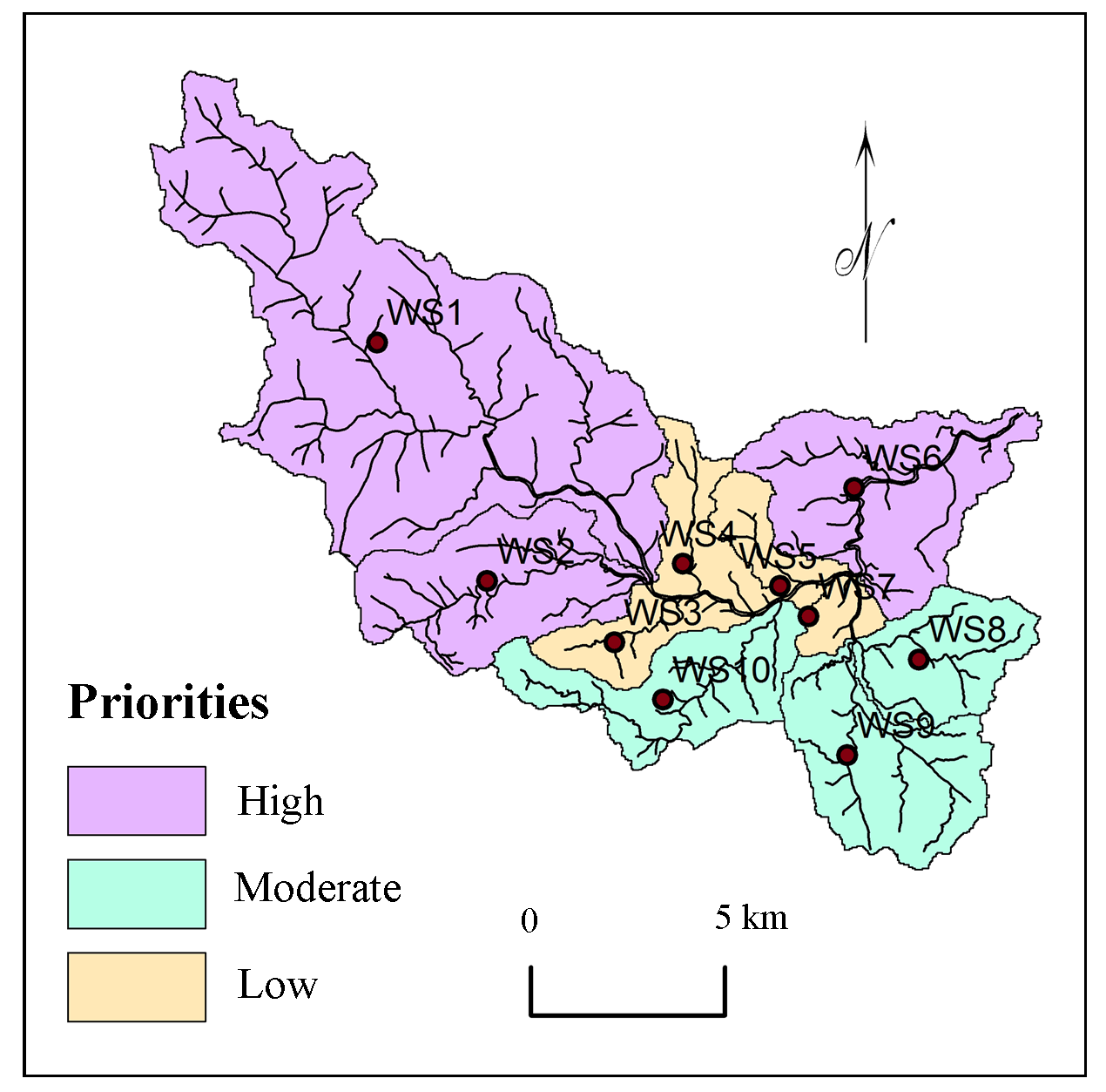
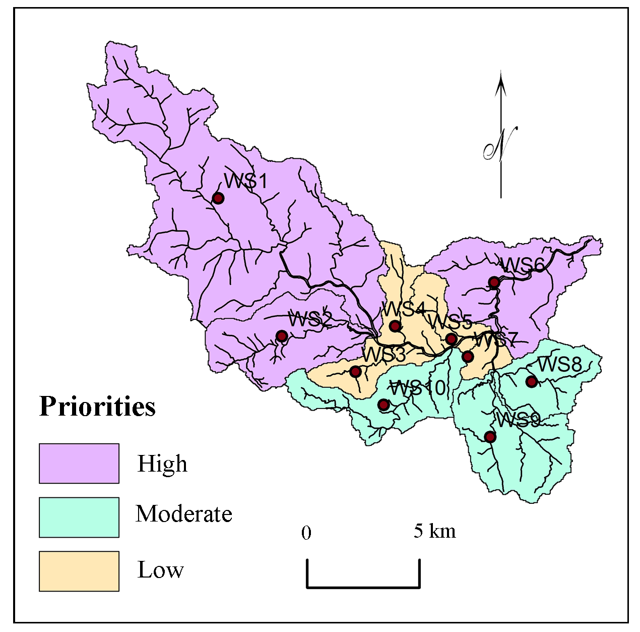
Priorities of sub-watersheds for planning and development were calculated using multi-criteria based AHP method and calculated influences of criterions. Morphometric and physiographic criterions (19) were selected and ranked using correlation analysis for estimations of weights and influences. Estimated influences of criterions were normalized based on spatial distribution in selected sub-watersheds for prioritization. Estimated priorities were classified into three classes (Figure 7): high, moderate and low priorities.
4.1 Highly Priority
Sub-watersheds, WS1, WS2 and WS6 with first, second and third priorities are classified into the class, ‘Highly priority’ for planning and management of resources (Figure 7). These watersheds have gentle to moderate slopes with very shallow extremely drained loamy calcareous soils and severe erosion activities (Table 9). The productivity of these soils is very low and natural resources are exploited.
4.2 Moderate Priority
Watersheds: WS8, WS9 and WS10 were classified into the class, ‘Moderate priority’. Gentle slopes (27.80% area), calcareous soils with moderate erosion observed in these watersheds. Bifurcation Ratio and Texture Ratio indicate more surface erodibility and runoff from the basin which supports to more surface erosion.
4.3 Low Priority
Watersheds: WS3, WS4, WS5 and WS7 show low drainage density, plain surface and low erosion activities with comparatively good agriculture. Well irrigation in rainy season is observed for commercial crops near to streams. Therefore, these watersheds are suggested with comparatively low priorities for planning and development.
5. Conclusion
- AHP based multi-criteria analysis is useful for prioritization of watersheds for planning, management and development.
- Nineteen criterion i.e.\(R_b\), \(L_b \), \(A\), \(L_b\), \(P\), \(D_d\), \(P\), \(F_s\), \(R_f\), \(R_e\), \(C_C\), \(D_t\), \(T\), \(D_i\), \(I_f\), \(R_{h1}\), \(R_n\), slope and soil were selected for prioritization of sub-watersheds in the region.
- Correlation analysis is useful for robust judgment for ranking the criterion for prioritization of selected watersheds.
- Drainage intensity (27.80%), texture ratio (13.90%), bifurcation ratio (9.27%), geology (6.95%) and basin length (5.56%) show higher influence on nature of watersheds in the region.
- Influences of criterion were estimated based on weights estimated using AHP methods. These values of influences are normalized using distribution of selected criterion within the sub-watersheds.
- Watersheds were classified into three categories of priorities: high, moderate and low priorities.
- The methodology formulated in this study can be efficient tool for rapid prioritization of watersheds for planning and management for development.
Conflict of interest
The authors declare no conflict of interest.
Acknowledgements
Anonymous reviewers thanked for useful comments and suggestions to improve the manuscript.
Abbreviations
AHP: Analytical Hierarchy Process; SOI: Survey of India; SW: Sub-Watershed.
Article information
- Received
- 30 Dec 2017
- Revised
- 8 Jan 2018
- Accepted
- 9 Jan 2018
- Published
- 21 Jan 2018
- Handling editor
- Dr. Pramodkumar Hire
- Licence
- CC BY-NC-ND 4.0
- Journal
- Hydrospatial Analysis, ISSN 2582-2969
References
-
Aher, P. D., Adinarayana, J. and Gorantiwar, S. D., 2014. Quantification of morphometric characterization and prioritization for management planning in semi-arid tropics of India: A Remote Sensing and GIS approach. Journal of Hydrology, 511, 850-860.
Crossref -
Ali, A., Esayas, A. and Beyene, S., 2010. Characterizing soils of Delbo Wegene watershed, Wolaita Zone, Southern Ethiopia for planning appropriate land management. Journal of Soil Science and Environmental Management, 1 (8), 184-199.
-
Ali, U., Ali, S. A., Ali, U., 2014. Analysis of drainage morphometry and watershed prioritization of Romushi-Sasar catchment, Kashmir Valley, India using Remote Sensing and GIS technology. International Journal of Advanced Research, 2(12), 5-23.
-
Ames, D. P. and Neilson, B. T., Stevens, D. K. and Lall, U., 2005. Using bayesian networks to model watershed management decisions: An East Canyon Creek case study. Journal of Hydroinformatics, 07(4), 267-282.
-
Aouragh, M. H. and Ali, E., 2014. Morphometric analysis of a Guigou sub-watershed, Sebou basin, Middle Atlas, Morocco using GIS based ASTER (DEM) image. International Journal of Innovative Research in Science, Engineering and Technology, 3(4), 11503-11512.
-
Aravinda, P. T. and Balakrishna, H. B., 2013. Morphometric analysis of Vrishabhavathi watershed using Remote Sensing and GIS. International Journal of Research in Engineering and Technology, 2(8), 514-522.
-
Argyriou, A.V., Teeuw, R. M., Rust, D., Sarris, A., 2016. GIS multi-criteria decision analysis for assessment and mapping of neotectonic landscape deformation: A case study from Crete. Geomorphology, 253(10), 262-274.
Crossref -
Bhagat, V. S., 2012. Use of Remote Sensing techniques for robust digital change detection of land: A review. Recent Patents on Space Technology, 2(2), 123-144.
Crossref -
Bhagat, V. S., 2013. Use of Remote Sensing techniques for robust detection and estimations of soil organic carbon: A review. Recent Progress in Space Technology, (3) 83-102.
Crossref -
Bhagat, V. S., 2014. Space-borne passive microwave Remote Sensing of soil moisture: A review. Recent Progress in Space Technology, (4) 2, 119-150.
Crossref -
Bhattacharyya, R., Ghosh, N., Mishra, P. K., Mandal, B., Rao, C. S., Sarkar, D., Das, K., Anil, K. S., Lalitha, M., Hati, K. M. and Joseph, F. A., 2015. Soil degradation in India: Challenges and potential solutions, Sustainability, 7(4), 3528-3570.
Crossref -
Bishop, M. P., James, L. A., Shroder, J. F., Walsh, S. J., 2012. Geospatial technologies and digital geomorphological mapping: Concepts, issues and research. Geomorphology, 137, 5-26.
Crossref -
Cannon, J., 2000. Choices and institutions in watershed management. William and Mary Environmental Law and Policy Review, 25(2), 379-428.
-
Capodici, F., Maltese, A, Ciraolo, G., La Loggia, G., D’Urso, G., 2013. Coupling two radar backscattering models to assess soil roughness and surface water content at farm scale. Hydrological Sciences Journal, 58 (8), 1677-1689.
Crossref -
Chang, H. K., Tan, Y. -C., Lai, J.-S., Pan, T.-Y., Liu, T.-M. and Tung, C.-P., 2013. Improvement of a drainage system for flood management with assessment of the potential effects of climate change. Hydrological Sciences Journal, 58 (8), 1581-1597.
Crossref -
Chatterjee, A. and Tantubay, A., 2000. Morphometric analysis for evaluating groundwater potential zones, in Kusangai Jor Watershed Area, Dist. Bolangir, Orissa. Department of Geology, Presidency College, 86/1 College Street, Kolkata-700073, 1-6.
-
Chitra, C., Alaguraja, P., Ganeshkumari, K., Yuvaraj, D. and Manivel, M., 2011. Watershed characteristics of Kundah sub basin using Remote Sensing and GIS techniques. International Journal of Geomatics and Geosciences, 2(1), 311-335.
-
Corn, M. L., 1993. Ecosystems, Biomass, and Watersheds: Definitions and Use. Washington DC, National Council for Science and the Environment.
-
Dhanalakshmi, V. and Shanmugapriyan, R., 2015. Assessment of quality of open well water and its suitability for human use in Pollachi, Coimbatore district, Tamilnadu, India. World Journal of Pharmaceutical Research, 4 (10), 1833-1841.
-
Elaalem, M., 2012. Land suitability evaluation for sorghum based on boolean and fuzzy-multi-criteria decision analysis methods. Int. J. Environ. Sci. Develop. 3 (4), 357-361.
Crossref -
Emamgholi, M., Khosravi, K. and Sedaii, N., 2007. Suitable site selections for Gabion Check dams construction using analytical Hierarchy Process and Decision Making methods. Journal of Soil Environment, 2(4), 170-179.
-
Engelhardt, B. M., Weisberg P. J. and Chambers, J. C., 2011. Influences of watershed geomorphology on extent and composition of riparian vegetation. Journal of Vegetation Science, 23(01), 127-139.
Crossref -
Evers, M. and Nyberg, L., 2013. Coherence and inconsistency of European instruments for integrated river basin management. Intl. J. River Basin Management, 11(2), 139-152.
Crossref - Crossref
-
Farhan, Y. and Anaba O., 2016. A Remote Sensing and GIS approach for prioritization of Wadi Shueib mini-watersheds (Central Jordan) based on morphometric and soil erosion susceptibility analysis. Journal of Geographic Information System, 8(14), 1-19.
-
Feizizadeh, B., Roodposhti, M. S., Jankowski, P. and Blaschke, T., 2014. A GIS-based extended fuzzy multi-criteria evaluation for landslide susceptibility mapping. Computers and Geosciences, 73, 208-221.
Crossref -
Ferrer, J. P., Foguet, A. P., Codony, J., Ravento, E. and Candela, L., 2014. Assessment of water resources management in the Ethiopian Central Rift Valley: environmental conservation and poverty reduction. International Journal of Water Resources Development, 30(3), 572-587.
Crossref -
Flint, L. E., Flint, A. L., Thorne, J. H. and Boynton, R., 2013. Fine-scale hydrologic modeling for regional landscape applications: The California Basin Characterization Model development and performance. Ecological Processes, 2(01), 1-25.
Crossref -
Gabale, S. M. and Pawar, N. R., 2015. Quantitative morphometric analysis of Ambil Odha (Rivulet) in Pune, Maharashtra, India. IOSR Journal of Environmental Science, Toxicology and Food Technology, 9(7), 41-48.
-
Gajbhiye, S., Sharma, S. K., Meshram, C., 2014. Prioritization of watershed through sediment yield index using RS and GIS approach. International Journal of u- and e- Service, Science and Technology, 7(6), 47-60.
-
Gashaw, T., Tulu, T. and Argaw, M., 2017. Erosion risk assessment for prioritization of conservation measures in Geleda watershed, Blue Nile Basin, Ethiopia. Environ Syst. Res, 6(1), 1-14.
Crossref -
Gebre, T., Kibru, T., Tesfaye, S. and Taye, G., 2015. Analysis of watershed attributes for water resources management using GIS: The case of Chelekot micro-watershed, Tigray, Ethiopia. Journal of Geographic Information System, l7(2), 177-190.
-
Ghanbarpour, M. R. and Hipe, K. W., 2011. Multi-criteria planning approach for ranking of land management alternatives at different spatial scales. Research Journal of Environmental and Earth Sciences, 3(2), 167-176.
-
Gharde, K. D. and Kothari, M., 2016. Hydromorphometric analysis and prioritization of Savitri Basin of Maharashtra, India using GIS. International Journal of Civil, Structural, Environmental and Infrastructure Engineering Research and Development (IJCSEIERD), 6(2), 1-10.
-
Gray, D. M., 1961. Interrelationships of watershed characteristics. Journal of Geophysical Research, 66(4), 1215-1223.
Crossref -
Gumma, M. K., Birhanu, Z., Mohammed, I. A., Tabo, R. and Whitbread, A. M., 2016. Prioritization of watersheds across Mali using Remote Sensing data and GIS techniques for agricultural development planning. Water, 8(260), 1-17.
Crossref -
Horton, R. E., 1945. Erosion development of streams and their drainage basins: Hydrophysical approach to quantitative morphology. Bulletin of the Geological Society of America, 56, 275-370.
Crossref -
Iqbal, M. and Sajjad, H., 2014. Watershed prioritization using morphometric and land use/land cover parameters of Dudhganga Catchment Kashmir valley India using spatial technology. Geophysics and Remote Sensing, 3(1), 1-12.
>
Crossref -
Iqbal, M., Sajjad, H. and Bhat, F. A., 2013. Morphometric analysis of Shaliganga sub-catchment, Kashmir valley, India using Geographical Information System. International Journal of Engineering Trends and Technology, 4(1), 10-14.
-
Jagadeesh, C. B., Shivakumaranaiklal, H. S. and Sitaram, N., 2014. Morphometric analysis of a Vrishabhavathi sub-watershed upstream side of Gali Anjaneya temple using Geographical Information System. International Journal of Research in Engineering and Technology, 3(7), 103-107.
-
Jankar, P. D. and Kulkarni, S. S., 2013. A case study of watershed management for Madgyal village. International Journal of Advanced Engineering Research and Studies, 2(4), 69-72.
-
Johnson, J. N., Govindaradjane, S. and Sundararajan, T., 2013. Impact of watershed management on the groundwater and irrigation potential: A case study. International Journal of Engineering and Innovative Technology (IJEIT), 2(8), 42-45.
-
Joshi, P. K., Vasudha, P., Shiferaw, B, Wani, S. P., Bouma, J. and Scott, C., 2006. Socioeconomic and policy research on watershed management in India synthesis of past experiences and needs for future research. SAT eJournal, 2(7), 1-81.
-
Kaur, M., Singh, S., Verma, V. K. and Pateriya, B., 2014. Quantitative geomorphological analysis and land use/ land cover change detection of two sub-watersheds in Ne Region of Punjab, India. The International Archives of the Photogrammetry, Remote Sensing and Spatial Information Sciences, 49(8), 371-375.
Crossref -
Kaushal, S, S. and Belt, K. T., 2012. The urban watershed continuum: Evolving spatial and temporal dimensions. Urban Ecosystem, 15, 409-435.
Crossref -
Kedareswarudu, U., Aravind, U. S., Chattopadhyay, M., 2013. Analysis of watershed characteristics and basin management using RS and GIS: A case study from upper Provenance of Karamana river, Trivendrum district, Kerala. International Journal of Remote Sensing and Geoscience (IJRSG), 2(1), 36-48.
-
Khadri, S. F. R and Thakur, N. G., 2013. Geomorphological investigations of Bor River Basin (Tributary of Pedi River) Amravati district, Maharashtra using Remote Sensing and GIS techniques. International Journal of Scientific and Engineering Research, 4(11), 1089-1098.
-
Khare, D., Mondal, A., Mishra, P. K., Kundu, S. and Meena, P. K., 2014. Morphometric analysis for prioritization using Remote Sensing and GIS techniques in a hilly catchment in the state of Uttarakhand, India. Indian Journal of Science and Technology, 7(10), 1650-1662.
-
Kiran, V. S. S. and Srivastava, Y. K., 2014. Micro watershed level water resource management based on three years runoff estimation using Remote Sensing and GIS techniques for Simlapal Block, Bankura, West Bengal, India. International Journal of Earth Science and Engineering, 7(1), 80-92.
-
Kulkarni, M. D., 2015. The basic concept to study morphometric analysis of river drainage basin: a review. International Journal of Science and Research, 4(7), 2277-2280.
-
Li, Z.,Yong, F., Zeng, G., Li, J., Zhang, Q., Yuan, Q., Wang, Y., Ye, F., 2009. Temporal and spatial characteristics of surface water quality by an improved universal pollution index in red soil hilly region of South China: A case study in Liuyanghe River watershed. Environmental Geology, 58(01), 101-107.
Crossref -
Maddahi, Z., Jalalian, A., Zarkesh, M. K., Honarjo, N., 2017. Land suitability analysis for rice cultivation using a GIS-based Fuzzy Multi-criteria Decision Making Approach: Central Part of Amol District, Iran. Soil and Water Res., 12(1), 29-38.
Crossref -
Mangrule, V. N. and Kahalekar, U. J., 2013. Watershed planning and development plan by using RS and GIS of Khultabad Taluka of Aurangabad District. International Journal of Information and Computation Technology, 3(10), 1093-1100.
-
Miller, V. C., 1953. A quantitative geomorphic study of Drainage Basin Characteristics in the Clinch Mountain Area. Virgina and Tennessee, Proj. NR 389-402, Technical report 3, Columbia University, Department of Geology, ONR, New York.
-
Mishra, S. S. and Nagarajan, R., 2010. Morphometric analysis and prioritization of sub-watersheds using GIS and Remote Sensing techniques: A case study of Odisha, India. International Journal of Geomatics and Geosciences, 1(3) 501-510.
-
Mitchella, B., Priddleb, C., Shrubsolec, D., Vealeb, B. and Walters, D., 2014. Integrated water resource management: Lessons from conservation authorities in Ontario, Canada. International Journal of Water Resources Development, 30(3), 460-474.
Crossref -
Montz, B. E., 2008. Introduction to the issue: The role of science in watershed management. Universities Council on Water Resources Journal of Contemporary Water Research and Education, 138, 3-6.
Crossref -
Nagal, S., Tignath, S., Pandey, A., 2014. Morphometric analysis of the Adwa River Basin, tributary of Belan River, India. International Journal of Advanced Technology and Engineering Research, 4(2), 39-45.
-
Nolan, B. T., Healy, R. W., Taber, P. E., Perkins, K., Hitt, K. J. and Wolock, D. M., 2007. Factors influencing groundwater recharge in the Eastern United States. Journal of Hydrology, 332(1-2), 187-205.
Crossref -
Nongkynrih, J. M. and Husain, Z., 2011. Morphometric analysis of the Manas River basin using Earth Observation Data and Geographical Information System Jenita. InternationalJournal of Geomatics and Geosciences, 2(2), 647-654.
-
Oel, P. R. van, Odongo, V. O., Mulatu, D. W., Muthoni, F. K., Ndungu, J. N., Ogada, J. O. and Veen, A. van der., 2014. Supporting IWRM through spatial integrated assessment in the Lake Naivasha Basin, Kenya. International Journal of Water Resources Development, 30(3), 605-618.
Crossref -
Olden, J. D., Kennard, M. J. and Pusey, B. J., 2012. A framework for hydrologic classification with a review of methodologies and applications in eco hydrology. Eco hydrology, 5(4), 503-518.
Crossref -
Pangare, V. L., 1998. Gender issues in watershed development and management in India. Agricultural Research and Extension Network, Network Paper, 88, 1-14.
-
Panhalkar, S., 2011. Land capability classification for integrated watershed development by applying Remote Sensing and GIS techniques. ARPN Journal of Agricultural and Biological Science, 6(4), 46-55.
-
Pareta, K. and Pareta, U., 2011. Quantitative morphometric analysis of a watershed of Yamuna Basin, India using ASTER (DEM) data and GIS. International Journal of Geomatics and Geosciences, 2(1), 248-269.
-
Patel, D. P., Gajjar, C., A. and Srivastava, P. K., 2013. Prioritization of Malesari mini-watersheds through morphometric analysis: A Remote Sensing and GIS perspective. Environmental Earth Sciences, 69(8), 2643-2656.
Crossref -
Perez, C. and Tschinkel, H., 2003. Improving watershed management in developing countries: A framework for prioritising sites and practices. Agricultural Research and Extension Network, 129, 1-14.
-
Pokharkar, D. V., 2011. A study of watershed development programme in Sangamner taluka: A geographical analysis. Unpublished Ph.D. Thesis.
-
Rai, P. K., Mohan, K., Mishra, S., Ahmad, A. and Mishra, V. N., 2014. A GIS-based approach in drainage morphometric analysis of Kanhar River Basin, India. Appl.Water Sci., 7(1), 217-232.
Crossref -
Raja, S. R. and Karibasappa, 2014. Suitable groundwater recharge structures in Noyyal River basin Coimbatore South Block using Remote Sensing and GIS. International Journal of Science and Research, 5(3), 1226-1231.
-
Ranjan, R., 2013. Saaty’s Analytical Hierarchical Process based prioritization of sub-watersheds of Bina River Basin using Remote Sensing and GIS. Thesis submitted to the Jawaharlal Nehru Krishi Vishwa Vidyalaya, Jabalpur, 3, 36-55.
-
Rao, A. K. and Yusuf, A., 2013. Morphomertic analysis for soil erosion assessment in parts of chambal basin using Remote Sensing and GIS, Madhya Pradesh. International Journal of Advanced Technology and Engineering Research, 3(3) 134-141.
-
Rao, N. K., Latha, S. P., Kumar, A. P. and Krishna, H. M., 2010. Morphometric analysis of Gostani River Basin in Andhra Pradesh State, India using spatial information technology. International Journal of Geomatics and Geosciences, 1(2), 189-187.
-
Rekha, V. B., George, A. V. and Rita, M., 2011. Morphometric analysis and micro-watershed prioritization of peruvanthanam sub-watershed, the Manimala River Basin, Kerala, South India. Environmental Research, Engineering and Management, 3(57), 6-14.
-
Rezaei, P., Rezaie, K., Nazari-Shirkouhi, S., Jamalizadeh, T. M. R., 2013. Application of Fuzzy Multi-Criteria Decision making analysis for evaluating and selecting the best location for construction of underground dam. Acta Polytechnica Hungarica, 10(7), 187-205.
-
Rockstrom, J., Folke, C., Gordon, L., Hatibu, N., Jewitt, G., Penning, de V. F., Rwehumbiza, F., Sally, H., Savenije, H. and Schulze, R., 2004. A watershed approach to upgrade rainfed agriculture in water scarce regions through Water System Innovations: An integrated research initiative on water for food and rural livelihoods in balance with ecosystem functions. Physics and Chemistry of the Earth, 29, 1109-1118.
Crossref -
Romshoo, S. A., Bhat, S. A. and Rashid, I., 2012. Geoinformatics for assessing the morphometric control on hydrological response at watershed scale in the Upper Indus Basin. Journal of Earth System Science, 121(3), 311-335.
Crossref -
Sepehr, A., Abdollahi, A., Mohammadian, A. and Nejad, M. P., 2017. Prioritization of Kashafrud sub-basins in terms of flooding sensitivity based on ELECTRE-TRI Algorithm. Universal Journal of Geoscience, 5(4), 83-90.
-
Shah, S. H. and Gibson, R. B., 2013. Research paper large dam development in India: Sustainability criteria for the assessment of critical river basin infrastructure. Intl. J. River Basin Management, 11(1), 33-53.
Crossref -
Sharma, S. K., Tignath, S., Gajbhiye, S. and Patil, R., 2009. Application of principal component analysis in grouping geomorphic parameters of Uttela Watershed for Hydrological Modeling. International Journal of Remote Sensing and Geoscience, 2(6), 1629-1634.
-
Shinde, V., Tiwari, K. N. and Singh, M., 2010. Prioritization of micro watersheds on the basis of soil erosion hazard using Remote Sensing and geographic information system. International Journal of Water Resources and Environmental Engineering, 2(3), 130-136.
-
Silva, da R. M., Santos, C. A. G., Silva, L. P. and Costa Silva, da J. F. C. B., 2007. Evaluation of soil loss in Guaraíra Basin by GIS and Remote Sensing based model. Journal of Urban and Environmental Engineering, 1(2), 44-52.
Crossref -
Singh, V. and Singh, U. C., 2011. Basin morphometry of Maingra River, district Gwalior, Madhya Pradesh, India. International Journal of Geomatics and Geosciences, 1(4), 891-902.
-
Smith, K. G., 1950. Standards for grading textures of erosional topography. American journal of Science, 248(9), 656-668.
Crossref -
Sridhar, P, Chandra, B., Giridhar, M. V. and Viswanadh, G. K., 2012. Prioritisation of mini-watersheds based on morphometric analysis using GIS. International Journal of Geomatics and Geosciences, 3(2), 314-320.
-
Strahler, A. N., 1957. Watershed geomorphology. Transactions - American Geophysical Union, 38(6), 913-920.
-
Strahler, A. N., 1964. Quantitative geomorphology of drainage basins and channel networks, in: Chow. V. T. (Ed.). Handbook of Applied Hydrology, Mc Graw-Hill, New York, 439-476.
-
Swallow, M. B., Johnson, N. L. and Meinzen Dick, R. S., 2001. Working with people for watershed management. Water Policy, 3, 449-455.
-
Swami, V. A., Kulkarni, S. S., Kumbhar, S. and Kumbhar, V., 2012. Participatory watershed management in South Asia: A comparative evaluation with special references to India. International Journal of Scientific and Engineering Research, 3(3), 1-9.
-
Tiwari, K. R., Bajracharya, R. M. and Sitaula, B. K., 2008. Natural resource and watershed management in South Asia: A comparative evaluation with special references to Nepal. The Journal of Agriculture and Environment, 9, 72-89.
Crossref -
Vandana, M., 2013. Morphometric analysis and watershed prioritisation: A case study of Kabani river basin, Wayanad district, Kerala, India. Indian Journal of Geo-Marine Sciences, 42(2), 211-222.
-
Vulevic, T., Dragovic, N., Kostadinov, S., Simic, S. B. and Milovanovic, I., 2015. Prioritization of soil erosion vulnerable areas using Multi-Criteria Analysis Methods. Pol. J. Environ, 24(1), 317-323.
Crossref -
Wani, S. P., Anantha, K. H., Sreedevi, T. K., Sudi, R., Singh, S. N. and D’Souza M., 2011. Assessing the environmental benefits of watershed development: Evidence from the Indian Semi-Arid Tropics. Journal of Sustainable Watershed Science and Management, 1(1), 10-20.
-
Wani, S. P., Sudi, R. and Pathak, P., 2008. Sustainable groundwater development through integrated watershed management for food security. International Crops Research institute for the Semi-Arid Tropics (ICRISAT) Patancheru PO, Andhra Pradesh, 502 324, India, 1-18.
-
Watson, N., 2014. IWR Min England: Bridging the gap between top-down and bottom-up implementation. International Journal of Water Resources Development, 30(3), 445-459.
Crossref -
Willett, I. R. and Porter, K. S., 2001. Watershed management for water quality improvement: the role of agricultural research watershed management for water quality improvement: The role of agricultural research. Aciar Working Paper, 52, 1-54.
-
Wilson, J. S., J., Chandrashekhar, N. and Magesh, N. S., 2012. Morphometric analysis of major sub-watersheds in Aiyar and Karai Pottanar Basin, Central Tamil Nadu, India using Remote Sensing and GIS Techniques. Bonfring International Journal of Industrial Engineering and Management Science, 2(1), 8-15.
-
Yeole, D., Patil, S. N. and Wagh, N. D., 2012. Evaluating pollution potential of irrigation by domestic wastewater on fertile soil quality of Mamurabad watershed area near Jalgaon Urban Centre, Maharashtra, India. Journal of Environment, 1(3), 84-92.
-
Yin, H., Udelhoven, T., Fensholt, R., Pflugmacher, D. and Hostert, P., 2012. How Normalized Difference Vegetation Index (NDVI) trends from Advanced Very High Resolution Radiometer (AVHRR) and Système Probatoire d’Observation de la Terre VEGETATION (SPOT VGT) time series differ in agricultural areas. An Inner Mongolian Case Study, Remote Sens., 4(11), 3364-3389.
Crossref -
Yunus, A. P., Oguchi, T. and Hayakawa, Y. S., 2014. Morphometric analysis of drainage basins in the Western Arabian Peninsula using multivariate statistics. International Journal of Geosciences, 5(5), 527-539.
Crossref -
Zeilhofer, P., Lima, G. A., Rondon L. E. B. and Santos, I., 2008. Development of a GIS-based information system for watershed monitoring in Mato Grosso, Central Brazil. Revista Pesquisas em Geociencias, 35(2), 23-37.
-
Zende, A. M., Nagarajan, R. and Atal, K. R., 2013. Prioritization of sub-watersheds in semi arid region, Western Maharashtra, India using Geographical Information System. American Journal of Engineering Research, 2(10), 28-135.
-
Zolekar, R. B. and Bhagat, V. S., 2015. Multi-criteria land suitability analysis for agriculture in hilly zone: Remote Sensing and GIS approach. Computers and Electronics in Agriculture, 118, 300-321.
Crossref