

Hydrospatial Analysis Volume 6 (2022), Issue 1-2 · pp. 54-72
Original Research Paper Open Access

Spatiotemporal Assessment of Meteorological Drought of Paschim Medinipur District, West Bengal, India

- Department of Geography, Bhairab Ganguly College, Feeder Road, Belghoria,Kolkata-700056, West Bengal, India.
* Corresponding author: Shrinwantu Raha, shrinwanturaha1@gmail.com
Contents
- Highlights
- Abstract
- 1. Introduction
- 2. Study Area
-
3. Methodology
- 3.1 Data Sources
- 3.2 Drought Evaluation Parameters (Dp)
- 3.2.1 Estimation of drought using Standardized Precipitation Evapotranspiration Index (SP…
- 3.2.2 Parameters Used in Drought Risk Assessment
- 3.2.2.2 Duration of drought (DD) using Run Theory
- 3.2.2.3 Magnitude (MD) and average intensity (MID) of drought
- 3.2.2.4 Occurrence rate (%) or frequency of drought (FD)
- 3.2.2.5 Mann Kendall trend test
- 3.2.2.6 Sen’s Slope estimator
- 3.3 Drought Susceptibility zone assessment by Principal Component Analysis (PCA)
- 4. Results
- 5. Discussion
- 6. Conclusion
- Conflict of interest
- Acknowledgements
- Abbreviations
- Article information
- References
-
- Figure 1. Study area
- Figure 2. Methodology
- Figure 3. Peak drought intensity
- Figure 4. Average drought intensity
- Figure 5. Spatial assessment of drought magnitude: a) 3 months, b) 6 …
- Figure 6. Spatial assessment of average duration of droughts: a) 3 mo…
- Figure 7. Spatial assessment of extreme to severe drought occurrence …
- Figure 8. Spatial assessment of moderate drought occurrence
- Figure 9. Mann Kendall trend of drought: a) 3 months, b) 6 months, c)…
- Figure 10. Sen’s slope of droughts
- Figure 11. Drought susceptibility zone assessment by Principal Compon…
-
- Table 1. Meteorological stations
- Table 2. Drought severity classes based on SPEI
- Table 3. Station-wise assessment of drought at 3 months
- Table 4. Station-wise assessment of drought at 6 months
- Table 5. Station-wise assessment of drought at 12 months
- Table 6. Station-wise assessment of drought at 48 months
- Table 7. Drought magnitudes
- Table 8. Estimated area under drought
Highlights
- Drought has been assessed spatio-temporally at 3 months, 6 Months, 12 Months and 48 Months.
- Peak intensity, average drought intensity, magnitude, occurrence rate (%) and trend, are considered here as the drought evaluation parameters.
- As the time step advances, peak intensity, magnitude, average drought intensity, Extreme to Severe drought occurrence rate starts to decrease in significant proportion.
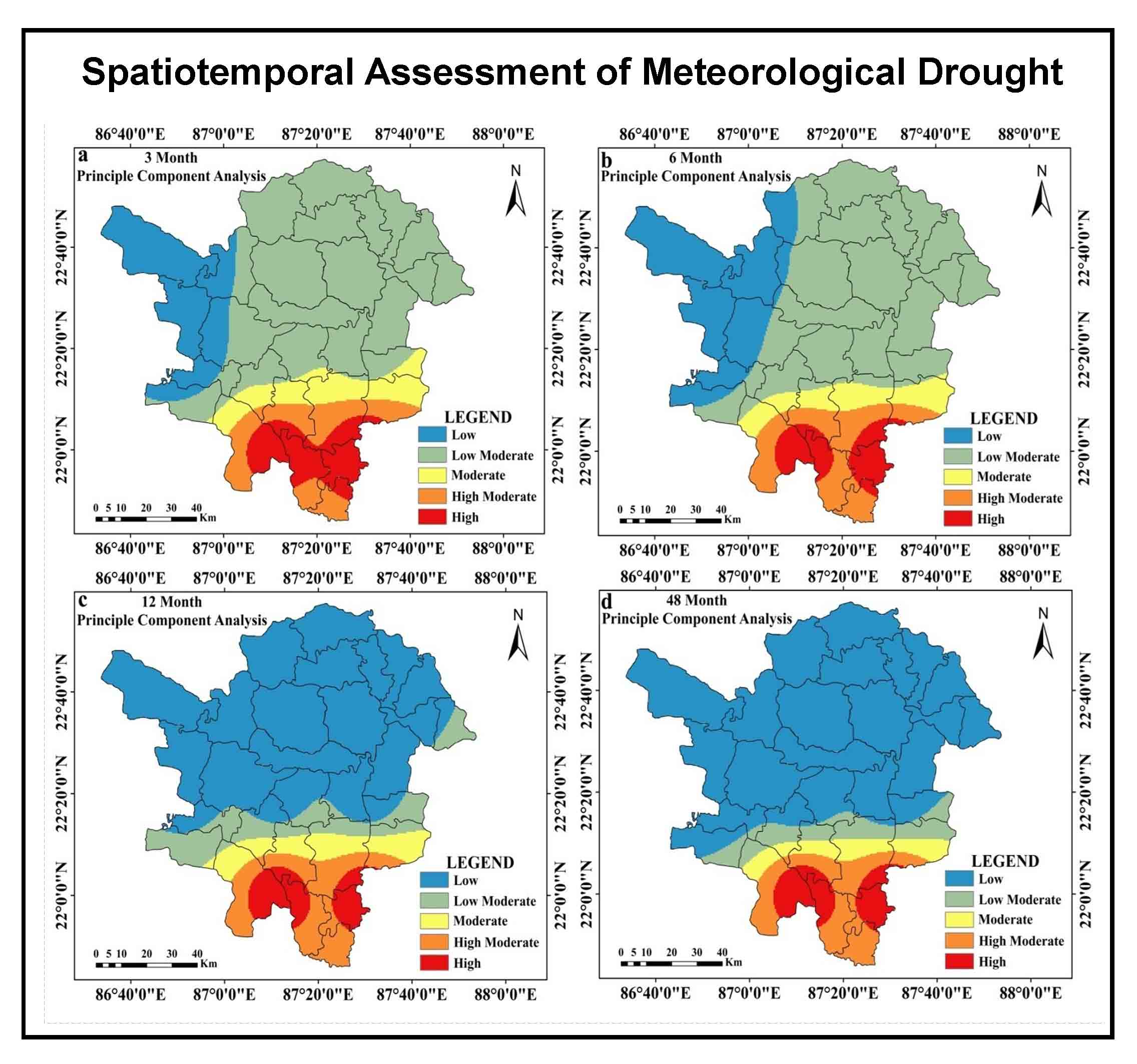
- Drought prone zones are demarcated using composite scores of PCA and those composite scores are estimated using the above-mentioned parameters at several time steps.
- Overall 16% area is found under high to high moderate drought prone category, whereas, approximately, 65% area is found under the low to low moderate drought category.
Abstract
The drought phenomenon is linked to the water scarcity and these are the pressing issues that require careful and thoughtful consideration. Drought in India mostly affects regions that are part of numerous plateaus, including the Chottanagpur plateau and the Deccan plateau. The Paschim Medinipur District of West Bengal, which is located in the southern portion of the Chottanagpur plateau, has recently experienced extreme and severe drought on multiple occasions. The assessment of the drought scenario in this region is, nevertheless, still very far from being finalized. Using the Standardized Precipitation Evapotranspiration Index (SPEI) at various time intervals (e.g., 3 months, 6 months, 12 months and 48 months) between 1979 and 2014, we have evaluated drought both geographically and temporally in this study. Here, the drought evaluation metrics include peak intensity, average intensity, magnitude, occurrence rate (%) and trend. Peak intensity, magnitude, average drought intensity, and the frequency of Extreme to Severe (ES) droughts are all seen to decline noticeably as time steps move forward. The frequency of moderate droughts starts to rise as time moves forward. Peak intensity, magnitude, average drought intensity, drought duration, ES and moderate drought occurrence rate is high in southern and southwestern portions of Paschim Medinipur. Additionally, the Principal Component Analysis (PCA) composite scores used to identify the drought-prone zones are estimated using the aforementioned parameters at various time steps. As the time step increases the area under the high and high moderate drought prone zone decreases, but very low and low drought prone area increases. Overall 16% area is found under high to high moderate drought prone category, whereas, approximately, 65% area is found under the low to low moderate drought category. The outcome of this research may be helpful to combat with drought and to make a fruitful move to manage water resources in the Paschim Medinipur region, West Bengal. Additionally, the study makes use of a superb methodology to comprehend the spatiotemporal variation of meteorological drought, which is applicable to all parts of the globe.
Keywords trendStandardized PrecipitationMeteorological DroughtEvapotranspiration Indexduration
1. Introduction
A region’s climate is determined by the long-term mean, regularity and extremes of a variety of climatological and meteorological factors (Durdu, 2010; Chanda et al., 2014). Drought is a recurring phenomenon that has detrimental effects on many different water related industries (Spinoni et al., 2014). It is typically regarded as the extended period with much less precipitation than average (Shadeed, 2013; Chanda et al., 2014). Meteorological drought is characterized by a lack of precipitation, which results in decreased water supply for residential and other uses (Gupta et al., 2011; Liu et al., 2015; Measho et al., 2019). In other words, an extended period of water scarcity can be used to characterize meteorological drought (Chhajer et al., 2015; Kar and Saha, 2012). Even though there are droughts worldwide, they vary in severity, length and frequency according to local factors and climatic zones (Mirabbasi et al., 2013; Kwon et al., 2019). In terms of spatiotemporal characteristics, which result in organized spatial coverage with variable durations, drought is significantly different from other water related risks (Kwon et al., 2019; Thomas et al., 2015). One of the most frequent climatic extremes that most people experience worldwide is drought (NRC, 2010; Yan et al., 2016; Guo et al., 2017; Sadeghi and Hazbavi, 2017; Mishra and Singh, 2011; Zarch et al., 2015). As a result, drought monitoring and early warning systems have become effective tools for reducing and averting the detrimental effects of drought at both the global and local levels (Kwon et al., 2019). More than 50% of India is at risk of drought (Kamble et al., 2010; Sonmez et al., 2005). Studies have employed a variety of indexes to try and explain drought events in different ways (Tefera et al., 2019; Zhang and Zhou, 2015). According to Svoboda and Fuchs (2016), drought indices bring numerical representation of intensity, frequency, duration and magnitude of drought. A lot of works has been done on spatiotemporal variation of drought using SPEI. For example, Musei et al. (2021) evaluate the spatiotemporal variation of meteorological drought over the Somalia using SPEI. They identify the major drought events of May 2011 and January 2013. Southern parts of Somalia are found with moderate to severe drought proneness. Bezdan et al. (2019) assess the agricultural drought of Carpethian Basin of Republic of Serbia using the SPEI. The Western portion of the Carpethian Basin is identified with the higher drought sensitivity. The Food and Agricultural Organization (FAO) and Soil Conservation Service of the US Department of Agriculture Method (USDA-SCS) based simple methodologies are used by Zarei and Moghimi (2019) to analyze the drought in the southwest of Iran. The Fasa, Drodzan and Zarghan meteorological stations are found with comparatively higher sensitivity to drought. Yang et al. (2016) used SPEI and GIS to analyze the spatiotemporal drought of Haihe River basin of China. The northern and central portions of the basin are found with comparatively higher drought proneness. Wang et al. (2018) evaluate the drought of the Yellow River Basin of China by utilizing the monthly data of 124 meteorological stations from 1961 to 2015. They have found that during the past 55 years the drought have increased significantly over this study area. SPEI is also used by Yang et al. (2019) to evaluate the characteristics of drought over the Yunnan Province, China. The drought frequency of the Zhaotong of the northeast China is highest with 36.53% occurrence rate. The central portion of the Yunnan province is found with comparatively low drought proneness. Apart from the above-mentioned researchers, Tong et al. (2018), Wang et al. (2015), Stagge et al. (2015), Xu et al. (2022) use the SPEI to specify the spatiotemporal drought phenomena at several locations of the world.
Further, there are several research outputs on spatiotemporal variation of meteorological drought using SPEI are also available from India. Alam et al. (2017) use the Markov model and three-dimensional log-linear models to simulate the SPEI over different agro-ecological regions of India. Six agro-ecological regions including the Eastern portions of India were marked with comparatively high drought sensitivity. Wable et al. (2018) evaluate the performance of different drought indices over the Sina River basin, Maharashtra, India and found that the increasing rate of drought proneness at the eastern portions of the study area. Bera et al. (2021) analyse the trends of variability of drought events over the Chottanagpur Plateau using SPI and SPEI indices at 3, 6, 12- and 48-months’ time steps. The year 1999, 2003, 2010, 2015 and 2016 are noticed with the extreme drought. This region is noticed with the 64% moderate drought occurrence rate. Saharwardi and Kumar (2022) assesse the drought in the homogeneous regions of India and found the increasing tendency in the eastern portions of India. Ghosh (2019) evaluates the drought of Gangetic West Bengal (GWB) using Standardized Precipitation Index (SPI), Geographical Information System (GIS) and multiple drought evaluation parameters and he found that north-western portions of the GWB are moderate to high drought-prone. Further, Ghosh (2018) evaluates the rainfall pattern at the Gangetic West Bengal and found that the Western and north-western portions of the GWB have immense scarcity of rainfall. Although, there are several research works are available on several parts of India and West Bengal, but the assessment of micro-level variability of drought in the Medinipur district is far from the conclusive statement till date. Further, Ghosh (2019) has stressed over the necessity of the micro-level variability of drought both at the short run and also for the long run. Therefore, the assessment of spatiotemporal variation of drought in the Paschim Medinipur district during 1979 to 2014 is a noble attempt.
In a big country like India, rainfall and temperature are important and vary both spatially and over time (Gupta et al., 2017). A new prediction states that by 2050, India’s overall water demand could increase by up to 32% (Mishra et al., 2015). Therefore, any decrease in precipitation patterns rarely causes a severe water crisis or increases the likelihood of a drought. One of the most well-known climatic limitations that affects the majority of people worldwide is dryness (NRC, 2010). Drought intensity has been seen in the northern hemispheres since the 1970s (Trenberth et al., 2014). In the tropics and subtropics, a similar trend has also been seen (Dai, 2011; Karavitis et al., 2011). Approximately 1391 million people have been affected by droughts in India between 1900 and 2016, according to statistics from CRED (2016). Recent evidence from West Bengal also supports the trend of increased susceptibility to drought (Khan et al., 2011). Paschim Medinipur and its surrounding regions ought to receive less rain during the monsoon season, according to Kar and Saha (2012). In Paschim Medinipur, the average temperature is predicted to climb by 1°C between 2025 and 2099 (Datta and Das, 2019; Dogan et al., 2012). In Paschim Medinipur for the past few years, the effects of climate change have been felt strongly and the advent of monsoon season has been delayed (Bhave et al., 2013). Additionally, it is noted that the population is growing and that the cultivation of hybrid seeds is dependent on irrigation water. Less prepared to deal with droughts is the Paschim Medinipur, which includes Gangetic West Bengal (GWB). In these circumstances, it seems sense to look into the spatiotemporal variance of the Paschim Medinipur meteorological drought.
2. Study Area
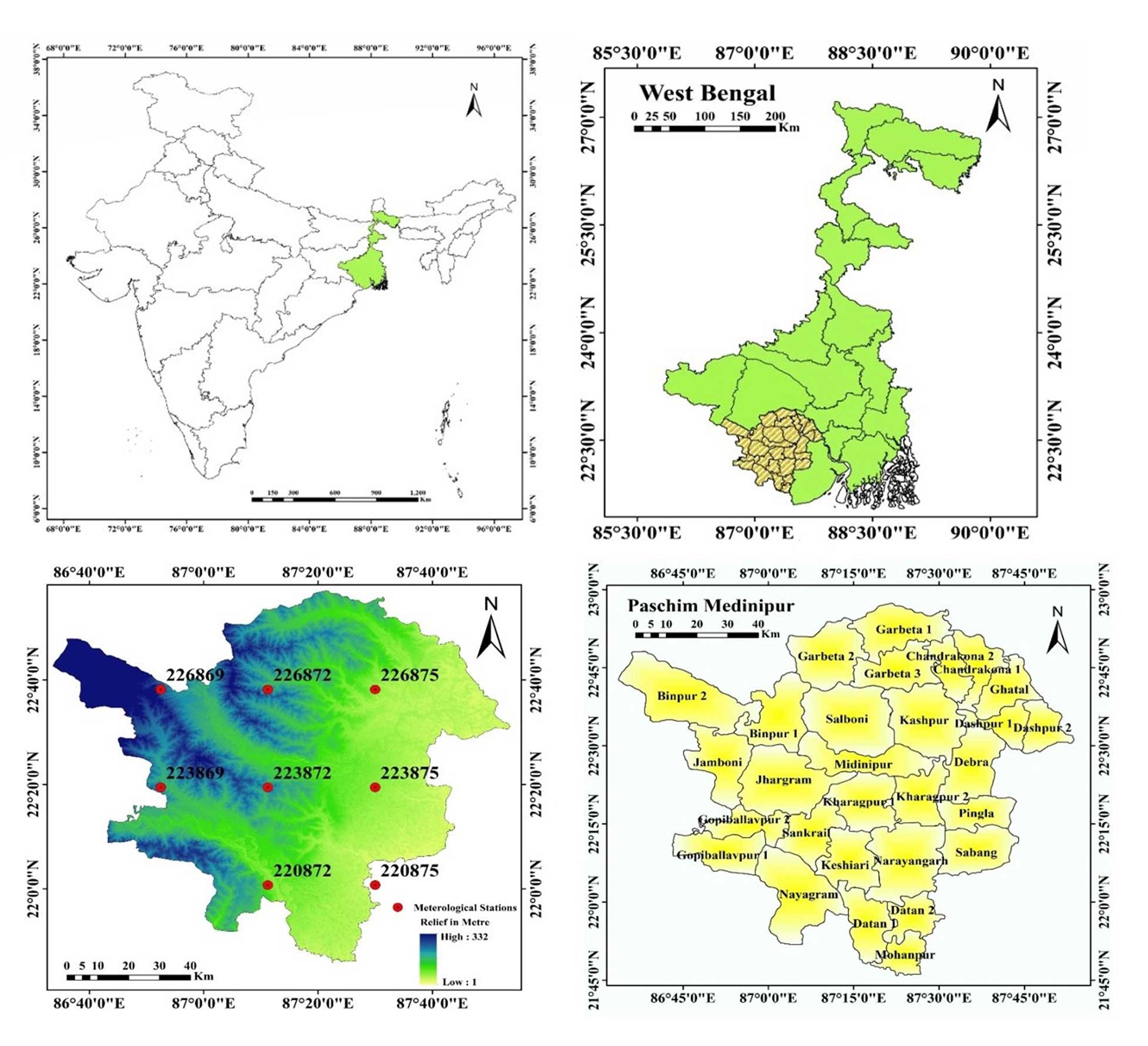
The district of Paschim Medinipur is situated in West Bengal’s southwest region (Figure 1). An extensive section of the degraded Chottanagpur Plateau is located to the region’s west. Kharagpur, Medinipur Sadar and Ghatal are the three subdivisions that make up the district. Kharagpur subdivision is made up of Kharagpur municipality and ten community development blocks, namely Dantan-I, Dantan-II, Pingla, Kharagpur-I, Kharagpur-II, Sabang, Mohanpur, Narayangarh, Keshiari and Debra. The Midnapore municipality and six community development blocks-Medinipur Sadar, Garhbeta-I, Garhbeta-II, Garhbeta-III, Keshpur and Shalboni- make up the Medinipur Sadar subdivision. Ramjibanpur, Chandrakona, Khirpai, Kharar and Ghatal are the five municipalities that make up the Ghatal subdivision, along with Chandrakona-I, Chandrakona-II, Daspur-I, Daspur-II and Ghatal.
3. Methodology
3.1 Data Sources
One of the most popular, reliable and adaptable dataset for identifying and monitoring droughts is CFSR (Sommerlot, 2017). CFSR data depends on both historical and operational archives of observations (White et al., 2017). Since 1978, many satellite missions are combined from CFSR assimilation which is from the archive of National Centres for Environmental Prediction (NCEP), European Centers for Environmental Prediction (ECMWF), Japan Meteorological Agency (JMA), United States Air Force (USAF) and African Monsoon Multidisciplinary Analysis (AMMA) (Dile and Srinivasan, 2014). Being the first reanalysis system to use the 6-hour prediction from a linked atmosphere-ocean climate system with an interactive sea ice component as the guess fields gives CFSR its singular advantage (Yu et al., 2011). The station data that is provided in the SWAT format at https://swat.tamu.edu/data/cfsr is created from the reanalysis datasets. These daily station data are extracted for our investigation and transformed to monthly values. The list of meteorological stations is shown in Table 1 together with their latitude, longitude, mean rainfall and standard deviation of rainfall. This study considers continuous rainfall data from 8 meteorological stations. Figure 1 shows where the meteorological stations are located in West Bengal’s Paschim Medinipur District. The overall methodological structure of this study is depicted in Figure 2. From rainfall and mean temperature, SPEI has been estimated. Based on SPEI intensity, magnitude, trend, duration and occurrence rate or frequency (%), are estimated at 3, 6, 12- and 48-months’ time step. The above-mentioned parameters are used to assess PCA at different time steps which is used to drought susceptibility zones of the study region.
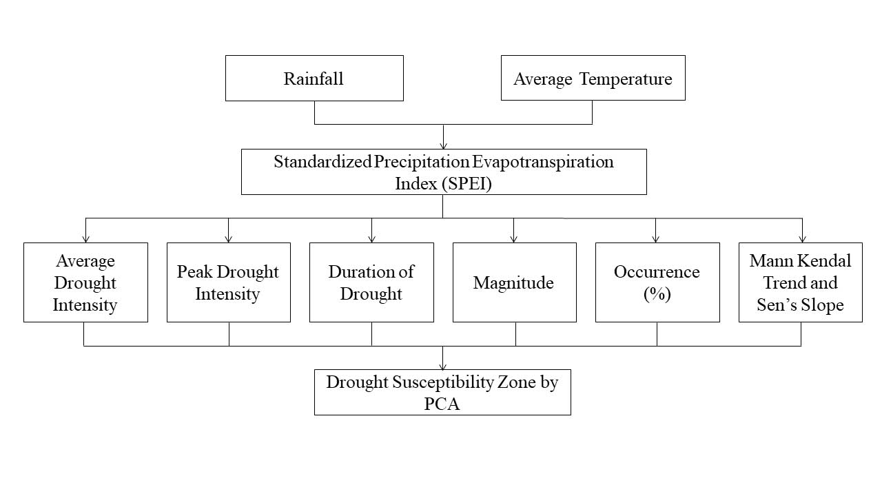
Table 1. Meteorological stations
|
Stations |
Longitude |
Latitude |
Elevation(m) |
|
220872 (1st Station) |
87.1875 |
22.0121 |
22 |
|
223872 (2nd Station) |
87.1875 |
22.3244 |
66 |
|
223875 (3rd Station) |
87.5 |
22.3244 |
12 |
|
226869 (4th station) |
86.875 |
22.6366 |
86 |
|
223869 (5th Station) |
86.875 |
22.3244 |
73 |
|
226872 (6th Station) |
87.1875 |
22.6366 |
63 |
|
226875 (7th Station) |
87.5 |
22.6366 |
15 |
|
220875 (8th Station) |
87.5 |
22.0121 |
9 |
3.2 Drought Evaluation Parameters (Dp)
Drought evaluation parameters are necessary to analyze drought in a meticulous way (Caloiero, 2018). Dracup et al. (1980) measured several drought related parameters such as intensity, frequency or occurrence rate, duration and trend of drought at several time steps. The manuscript follows almost same guideline to illustrate spatiotemporal assessment of meteorological drought:
3.2.1 Estimation of drought using Standardized Precipitation Evapotranspiration Index (SPEI)
According to Vicente-Serrano et al. (2010) and Beguera et al. (2013), the SPEI is based on temperature and precipitation data and has the advantage of integrating multi-scalar character with the ability to account for the effects of temperature fluctuation on drought evaluation. A climatic water balance, the accumulation of deficit/surplus at various time scales and adjustment to a log-logistic probability distribution are all steps in the process of calculating the index. The SPEI is mathematically comparable to the Standardized Precipitation Index (SPI), but it also takes temperature into account. The Palmer Drought Severity Index can be compared to the SPEI because it is based on a water balance (PDSI).
The SPEI generally utilizes monthly or weekly differences of rainfall and potential evapotranspiration (Thornthwaite, 1948). This phenomenon indicates a simple climatic water balance that can be calculated in different time steps which indicate SPEI. The first step of calculating SPEI involves the calculation of Potential Evapotranspiration (PET). Here the simple approach of Thornthwaite (1948) has been followed. The method has a great advantage that the method requires only the monthly mean temperature data. The monthly PET for this study is computed as follows:
\(PET= 16K({10T \over I})^m\) (1)
Where, T is the monthly mean temperature (°C), I is the heat index which is calculated as the sum of 12 monthly index values I, now the I is derived as following:
\(I= ({T \over 5})^{1.514}\) (2)
With the value of PET, the difference between the rainfall (P) and potential evapotranspiration (PET) for the month of i is calculated using following formula
\(D_i=P_i-PET_i\) (3)
The equation (3) gives the simple measure to estimate the surplus and deficit of the specific analyzed month.
In the next step of the SPEI formation D value is calculated in different time steps. The procedure of calculation of D is as follows:
\(X_{i,J}^K=∑_{l=13-K+l}^{12}D_{i-1J}+∑_{i=1}^j D_{iJ} \ if \ j<k \ and \ X_{i,J}^K=∑_{l=j-k+1}^j D_{i,l} \ {if} \ j≥k\) (4)
The equation (4) represents the total difference over one month in a certain year i using a 12-month time frame. The P-PET difference in millimeters during the first month of the year is represented here by Di. Depending on the time scale k used.
The series D has negative values so two parameters gamma distribution function cannot be fit for this series. Thus, three parameters gamma distributions have been used. In the three parameters gamma distribution x can take values in the range ( \(\gamma\) >D<\(\infty\)) where, \(\gamma\) is the parameter of origin of the distribution; consequently, x can have negative values which is common in the D series. After examining the 3-parameters gamma distribution function Vicente Serrano (2010) concluded that the log-logistic distribution is the best fit on the x series values. The form of the density function of the 3-parameters log-logistic distribution is expressed as follows:
\(f(x) = {β \over α} ({ x- \gamma \over α}) ^{β-1} [1+ ({ x- \gamma \over α})^β]^{-2}\) (5)
Where, α, β, \(\gamma\) are shape, scale and origin parameters respectively for D values ( \(\gamma\) >D<\(\infty\)). Here, x is the cumulative series of D values in a time window which is specified here as 1979-2014. The parameters of this function are obtained using the L moment method:
\(β = {2w_1-w_0 \over 6w_1-w_0-6w_2}\) (6)
\(α= {(w_0-2w_1)β \over ϊ(1+{1\overβ})ϊ(1-{1 \over β})}\) (7)
\(\gamma = w_0-α ϊ {(1+{1\overβ})ϊ(1-{1 \over β})}\) (8)
Where, \(ϊ \) is gamma function and the probability weighted moments are w0, w1, and w2. The equation (9) calculates the log-logistic cumulative distribution function is converted to the SPEI (10) using the Abramowitz and Stegun (1964) approximation of the standard normal distribution.
\(F'(x)= {1+ ({α \over x- \lambda})}\) (9)
\(SPEI=W- {C_0+C_1 W+C_2 W^2\over 1+d_1 W+W^2 d_2+w^3 d_3}\) (10)
Where, \(C_0,C_1,C_2,d_1,d_2\) and \(d_3\) are the constants in the SPEI equation constants and W is the obtained in the following equation (11):
\(W= \left\{ {\sqrt{-2In(P)} \over \sqrt{-2In(P-1)}} \right\} \) for \(p ≤ 0.5\), p>0.5 (11)
Where, P = 1- F(x). This index is able to monitoring drought with great amusement. Table 2 determines the category of drought and their respective ranges.
Table 2. Drought severity classes based on SPEI
|
Severity Class |
Nature of Drought |
|
<-2.0 |
Extremely dry |
|
-1.5 to -1.99 |
Severely dry |
|
-1.0 to -1.49 |
Moderately dry |
|
-.99 to .99 |
Near Normal |
|
1.0 to 1.49 |
Moderately Wet |
|
1.5 to 1.99 |
Very Wet |
|
>2.0+ |
Extremely Wet |
3.2.2 Parameters Used in Drought Risk Assessment
This study considers peak intensity, magnitude, average drought intensity, duration, occurrence rate and trend for evaluation of meteorological drought. Peak intensity (PID), magnitude (MD), average intensity (AID), duration, occurrence rate and trend are proportionately related with sensitivity of drought. Trend of drought is inversely related to drought sensitivity. The description of parameters is as follows:
3.2.2.1 Drought Intensity (ID)
According to Dupigny-Giroux (2001), drought intensity can be defined as the departure (down) of a SPEI from its typical value. A drought event, as described by Abbasi et al. (2019), is a time period during which the SPEI is consistently negative and the SPI achieves a value of -1.0 or less. Therefore, ID here signifies the SPEI value that is smaller than 1.0. The intensity of the drought will increase as SPI value decreases.
3.2.2.2 Duration of drought (DD) using Run Theory
Spinoni et al. (2014) use run theory to precisely quantify the length of a drought. When the SPEI is constantly negative and reaches to intensity of -1.0 or below, a drought event begins and it ends when the SPEI turns positive. Therefore, the continuous negative dimension of SPEI represents the length of the drought (Abbasi et al., 2019).
3.2.2.3 Magnitude (MD) and average intensity (MID) of drought
According to Thompson (1999), drought magnitude refers to the cumulative water deficit into the drought period. The average of this cumulative water deficit is the MID. Thus, MD is the sum of all SPEI values during the drought event and MID of a drought event refers to the magnitude of drought divided by the duration of the drought.
\(M_D=∑_(i=1)^n SPEI_{ij} \) (12)
\(M_D=∑_(i=1)^n SPEI_{ij} /m\) (13)
Where, SPEIij are the SPEI values of drought and wet event in j-th time and m is the number of months.
3.2.2.4 Occurrence rate (%) or frequency of drought (FD)
The number of droughts per 35 years calculated using following formula (Ghosh, 2019):
\(F_{Dj,35} = {M_j \over J.m} \times 100\) (14)
Where, FDj,35 is the frequency of droughts for timescale j in 35 years; Nj is the number of months with droughts for time scale j in the n-year set; j is time scale (3-, 6-, 12-, 48-months); n is the number of years in the data set.
3.2.2.5 Mann Kendall trend test
There are numerous statistical techniques available for identifying trends and each technique has strengths and weaknesses (Nikzad Tehrani et al., 2019). Finding the trend of meteorological variables can be done using the Mann-Kendall statistical test (Halder et al., 2020). Here, the tendency of a meteorological drought based on SPI is indicated by the Mann-Kendall trend test. One type of non-parametric test, the Mann Kendall test, is unaffected by the extremes of the sample points (Abeysingha and Rajapaksha, 2020). The World Meteorological Organization recommends the Mann-Kendall test (Mann, 1945; Kendall, 1975) and this approach is employed in the following way:
\(S=∑_{i=1}^{n-1}∑_{j=i+1}^n sgn(x_j-x_i)\) (15)
Where, n is the number of data points, xi and xj are the data values of the separate time series i and j (j>i) respectively, and \(sgn(x_j-x_i)\) is the sign function
\(sgn(x_j-x_i ) = \left\{ \begin {matrix} +1 \ if \ x_j-x_i>0 \\ 0 \ if \ x_j-x_i=0 \\ -1 \ if \ x_j-x_i=0 \end{matrix} \right \} \) (16)
The variance is computed as following:
\(Var(S) = {n(n-1)(2n+5)-∑_{i=1}^p t_i (t_i-1)(2t_i+5) \over 18}\) (17)
The summation sign denotes the sum of all tied groups, where n is the number of data points and P is the number of tied groups. The standard normal format of Zs can be computed in cases where the sample size is greater than 30, as shown below:
\(Z = \left\{ \begin {matrix} {s-1 \over \sqrt{var(s)}} \ if \ s>0 \\ 0 if \ s=0 \\ {s-1 \over \sqrt{var(s)}} \ if \ s>0 \end{matrix} \right \} \) (18)
Negative Zs value shows a positive tendency of drought, while positive Z value suggests a negative trend. Trends are tested using a defined degree of significance. When the null hypothesis is rejected, a substantial trend in the data series is present.
In the ARCGIS 10.2.2 environment, the Inverse Distance Weightage Method (IDW) has been used to visualize geographic maps.
3.2.2.6 Sen’s Slope estimator
The magnitude of trend in SPI time series was estimated in the following way (Theil, 1950; Sen, 1968):
\(β=median {X_i-X_j \over i-j}\) V \( j<i\) (19)
In the above equation (15), 1 < j < i < n. The β is the median over all combination of all recorded pairs (Tabari et al., 2011) thus does not affected by the extreme values in the observations.
3.3 Drought Susceptibility zone assessment by Principal Component Analysis (PCA)
One of the best and most widely used methods for calculating drought risk zones is Principal Component Analysis (PCA) (Cai et al., 2015; Dinpashoh et al., 2004). According to Demar et al. (2013), PCA is a multivariate technique that lowers the dataset’s dimensionality by computing a collection of new orthogonal variables in decreasing order. In order to estimate principal components, the research used Jolliffe’s (2002) method. In this work, the estimation of the principal components is done in time steps of 3, 6, 12 and 48 months. X is taken to be a vector made up of p random variables in this instance.
PCA is focused with the association and covariance in this investigation. A vector of p constants, such as α11, α12, . . ., α1p, and α′ is one of the constants in the linear function α′'x of the elements of x with the greatest variance, where ′ stands for transpose, so that
\(α'x= α_{11} x_1+α_{12} x_2+α_{13} x_3+⋯ +α_{1p} x_1=∑_{j=1}^p α_{1j} x_j\) (19)
So, the overall steps of the PCA are followed in the following
First step is to generate new PCA scores:
\(M(k)=(M_1………….M_p)_{(k)}\) (20)
This map a new vector Y(i) of X to a new vector of PCA scores:
\(L_{k(i)}=(L_1……….L_k)_i\) (21)
\(L_{k(i)}=Y_{i.} M_k\) (22)
Where, L is the maximum possible variance for Y which is a loading vector, M contained to be the unit vector. Here according to Jolliffe (2002), M1 has to satisfy the following condition
\(M_1=1^{argmax} \{∑_iY_i M^2 \}\) (23)
After certain modifications the following version are generated
\(M_1=1^{argmax} \{ {M^L Y^L Y_L \over M^T M} \}\) (24)
M1 equivalently satisfies the following condition
\(M_1={argmax} \{ {M^L Y^L Y_L \over M^T M} \}\) (25)
A standardized result of systematic matrix such as yTy is that the quotiont’s maximum possible value is the largest Eigen value of the matrix which occurs when M is the corresponding Eigen vector. When M1 is found the first component of the data vector Y(i) will be given a score.
\(M_{1(i)}=y_i.M_i\) (26)
The k-th component of the data vector will be given a score
\(L_{k(i)}=y_i.M_i\) (27)
Where, Mk is the kth eigen vector of the dataset yTy. So, the PCA decomposition of Y can be given as
\(l=yW \) (28)
The success of PCA is due to following two optional properties (Zou et al., 2006):
- Maximum variability in the given dataset can be captured by the Principal Component Analysis which incorporates minimum information loss.
- Since main components are mutually independent, it is possible to discuss one without mentioning others.
4. Results
4.1 Station-wise Comparison of Drought at 3 Months and 6 Months’ Time Step
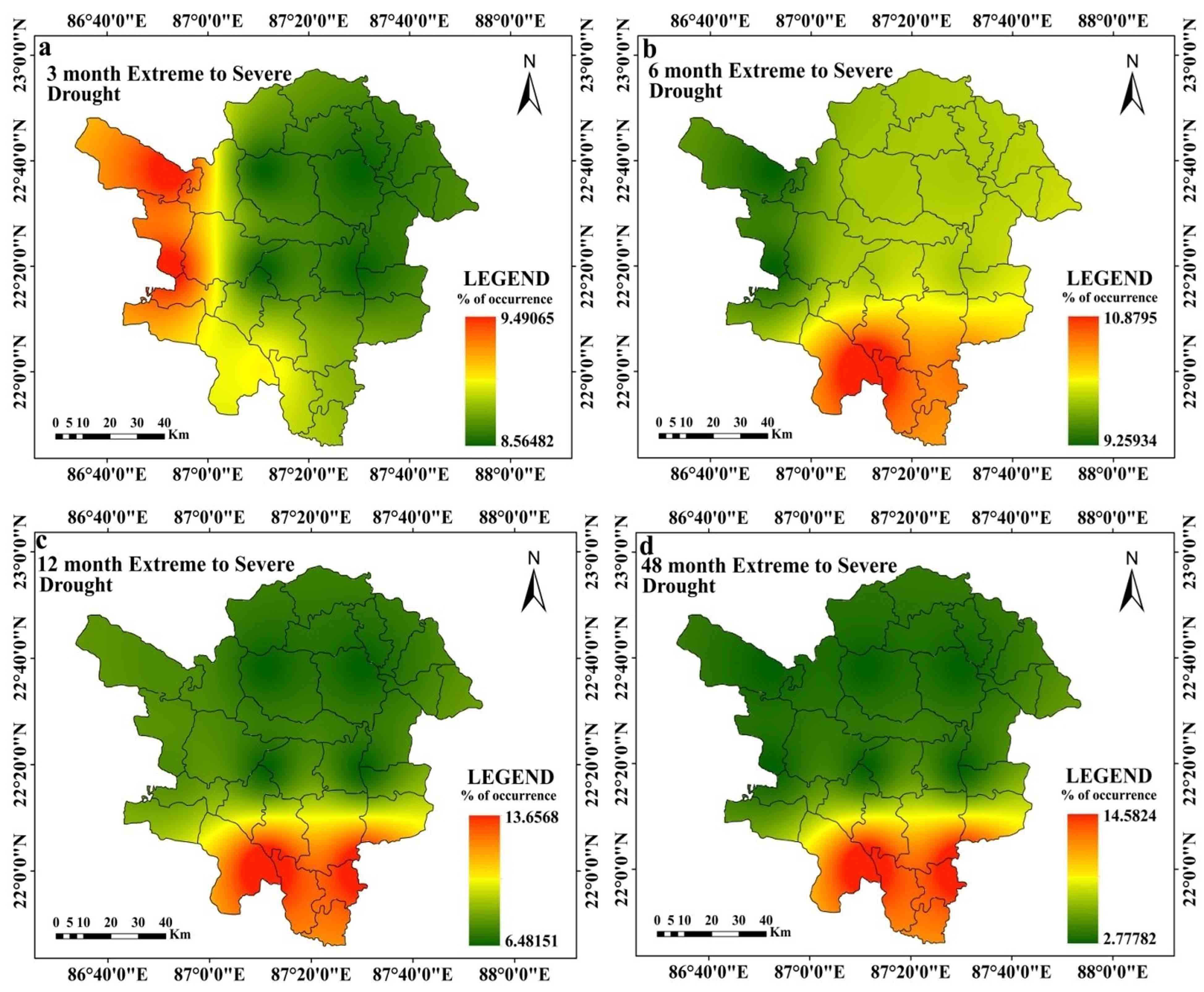
At 3 months’ time step, drought is at its’ peak (PID value -3.39) in 226869 (4th station) and 223869 station (5th Station) at January 2009 (Table 3). Other 5 stations experience highest drought intensity with below -2 PID value (station 220872, 220875, 226875, and 226872 respectively). Drought is observed at its’ highest intensity in post monsoon period. At 3 months’ time step, average drought is intensified in stations 226869 (4th Station) and 223869 (5th Station) with -1.56 AID value. Overall for all station average intensity is outlined with –1.51 value (Table 3). At this time step, 220872 (1st station) and 220875 station (8th Station) experiences highest drought magnitude (MD) with -135.96 SPEI value (Table 7). Drought (SPEI≤-1.0) magnitude at 3 months’ time step ranges between -113.82 to -135.96 value (Table 7). Extreme to severe (ES) drought is noticed with the highest rate of occurrence (9.49%) at 226869 (4th Station) and 223869 station. Overall, all of the meteorological stations are noticed with 8.56% to 9.49% ES drought (SPEI≤-1) occurrence rate. Moderate drought is observed with the highest rate of occurrence (~16%) at station 220875 (8th Station). Overall, moderate drought is noticed with 12% occurrence rate. All stations are observed with negative MK test, and Sen’s Slope value, which indicates that drought is intensified in these meteorological stations. However, the situation slightly alters at the 6 months time step. At a six-month time step, the drought peaked in March 2009 at stations 226869 (4th Station) and 223869 (5th Station), both of which had SPEI values of -3.63 (Table 4). All other stations are identified at this time step with PID values lower than -2. The pre-monsoon and late monsoon phases of the monsoon have the highest levels of drought intensity at this time step for practically all meteorological sites. Combining all station wise assessment, average intensity is noted with -1.49 SPEI value. Average intensity is highest at stations 226869 (4th Station) and 223869 (5th Station) with -1.56 SPEI value (Table 4). At this time step, highest drought magnitude (MD) is noticed with -129.83 value at station 220872 (1st Station) and 220875 (8th Station) (Table 7). At this time step, highest ES drought (10.88% occurrence rate), occurs at station 220872 (1st station). Moderate drought occurrence rate is highest (14.12% occurrence rate) at station 220875 (8th station). ES and moderate drought occurrence rate are lowest at station 226869 (4th Station) and 223869 (5th Station). Average ES and moderate drought occurrence rate are observed with 11.45% and 9.83% occurrence rate respectively.
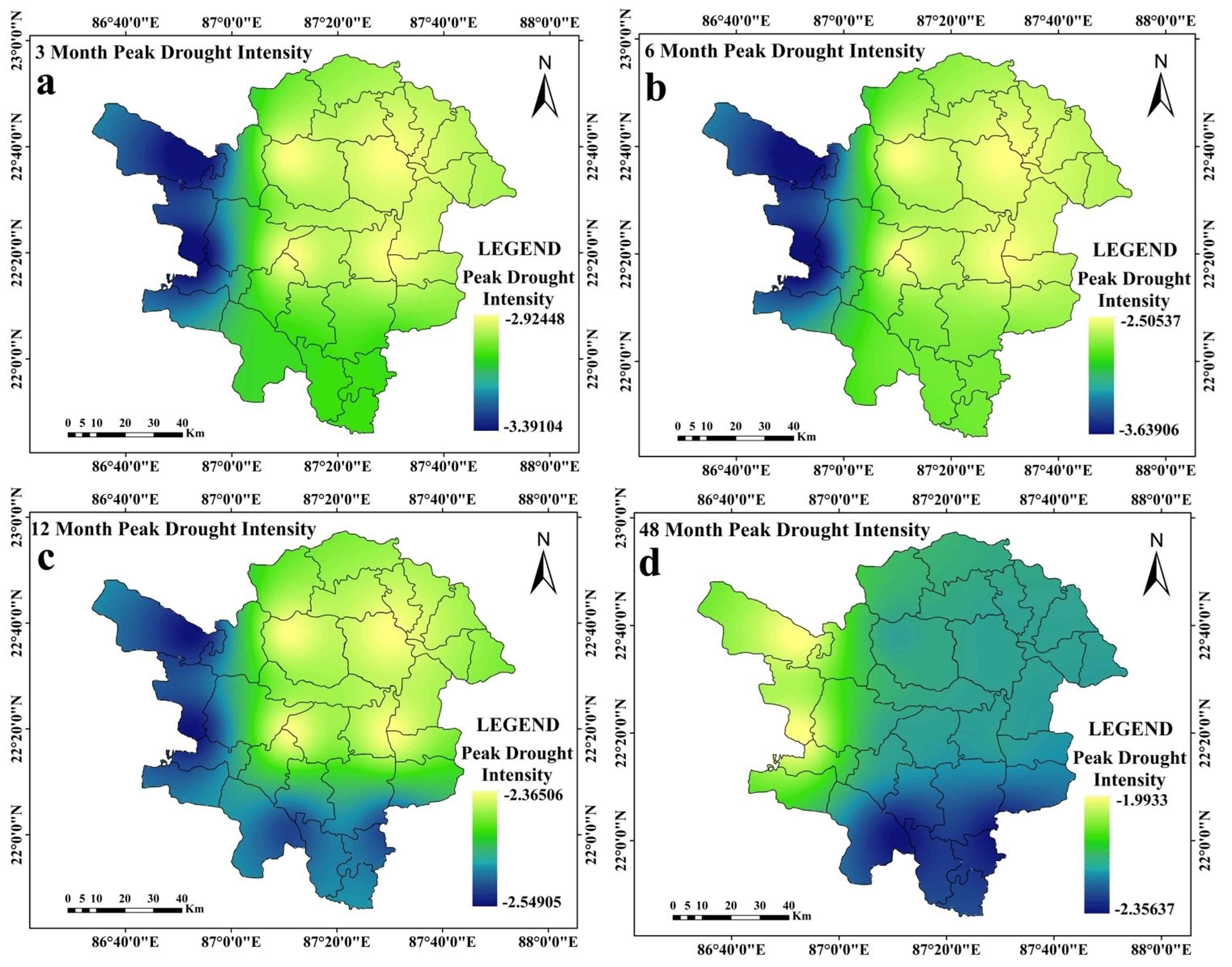
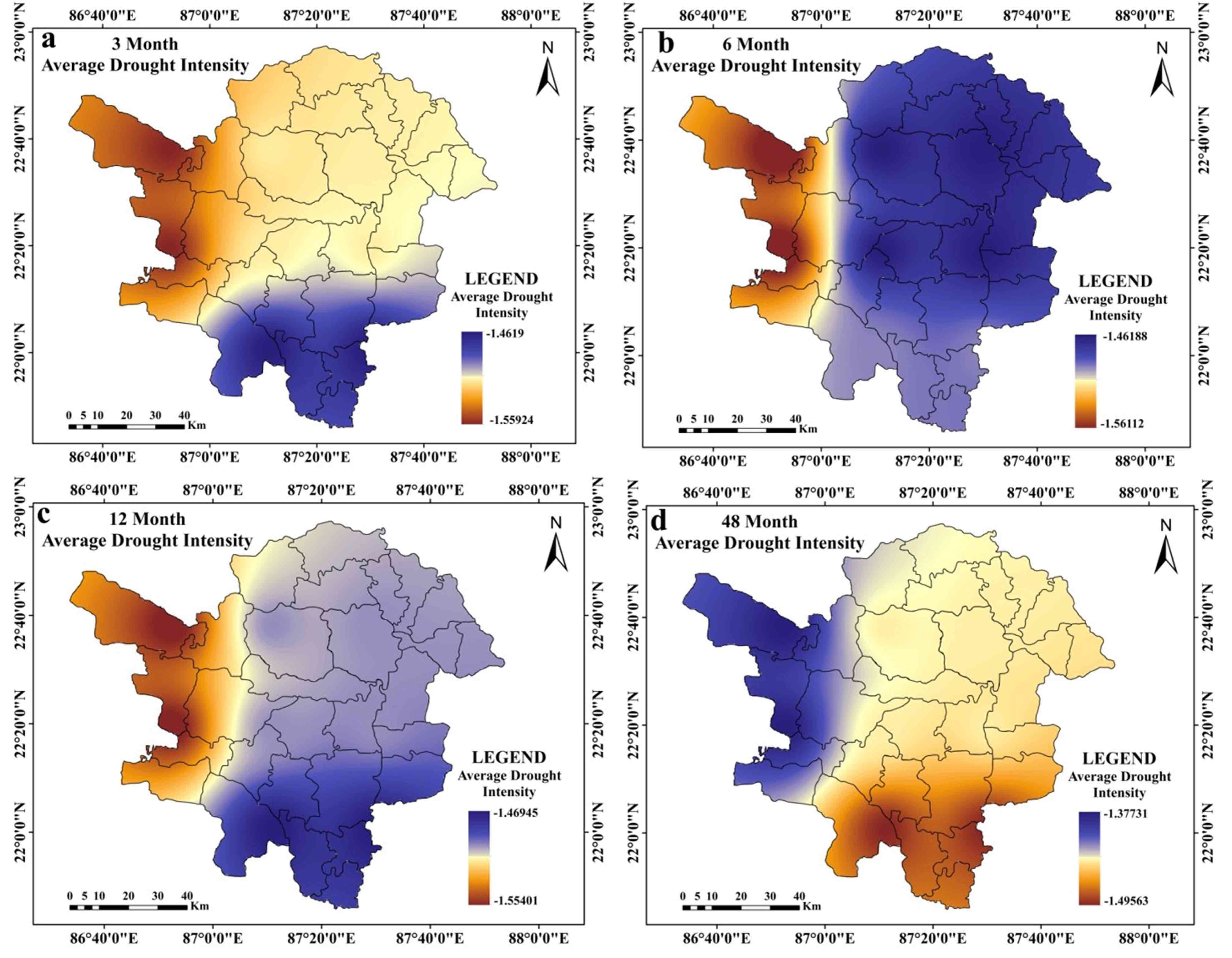
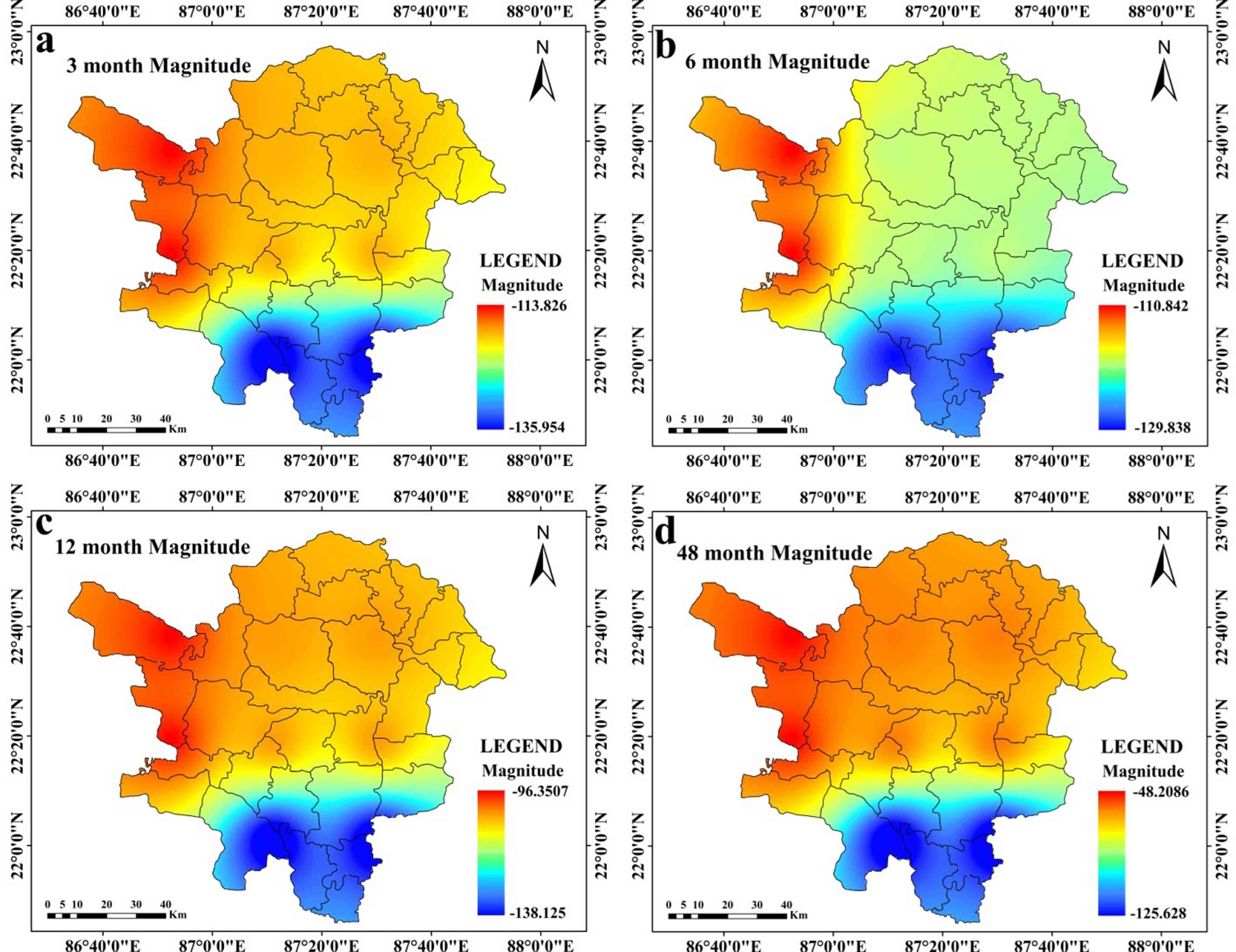
Table 3. Station-wise assessment of drought at 3 months
|
Stations |
Peak intensity (PID) |
Peak intensity observed |
Moderate drought occurrence rate |
Extreme to severe (ES) drought occurrence rate |
Average drought intensity (AID) |
Mann-Kendall trend |
Sen’s slope* |
|
220872 (1st station) |
-3.08 |
January-2009 |
15.74 |
9.03 |
-1.46 |
-0.04* |
-0.48* |
|
223872 (2nd Station) |
-2.92 |
January-2009 |
12.27 |
8.56 |
-1.51 |
-0.03* |
0.43 |
|
223875 (3rd Station) |
-2.92 |
January-2009 |
12.27 |
8.56 |
-1.51 |
-0.03* |
-0.43* |
|
226869 (4th Station) |
-3.39 |
January-2009 |
10.88 |
9.49 |
-1.56 |
-0.02 |
0.26 |
|
223869 (5th Station) |
-3.39 |
January-2009 |
10.88 |
9.49 |
-1.56 |
-0.02* |
-0.26* |
|
226872 (6th Station) |
-2.92 |
January-2009 |
12.27 |
8.56 |
-1.51 |
-0.03 |
0.43 |
|
226875 (7th Station) |
-2.92 |
January-2009 |
12.27 |
8.56 |
-1.51 |
-0.03* |
-0.43* |
|
220875 (8th Station) |
-3.08 |
January-2009 |
15.97 |
8.80 |
-1.46 |
-0.04* |
-0.48* |
*At 0.05 significance level
Table 4. Station-wise assessment of drought at 6 months
|
Stations |
Peak intensity (PID) |
Peak intensity observed |
Moderate drought occurrence rate |
Extreme to severe (ES) drought occurrence rate |
Average drought intensity (AID) |
Mann-Kendall trend (MK) |
Sen’s (S) slope |
|
220872 (1st Station) |
-2.76 |
March-2009 |
13.66 |
10.88 |
-1.49 |
-0.03* |
-0.24* |
|
223872 (2nd Station) |
-2.51 |
August-2010 |
10.88 |
9.72 |
-1.46 |
-0.02* |
-0.41 |
|
223875 (3rd Station) |
-2.51 |
August-2010 |
10.88 |
9.72 |
-1.46 |
-0.02* |
-0.41 |
|
226869 (4th Station) |
-3.64 |
March-2009 |
10.19 |
9.26 |
-1.56 |
-0.01 |
-0.07* |
|
223869 (5th Station) |
-3.64 |
March-2009 |
10.19 |
9.26 |
-1.56 |
-0.01 |
0.07 |
|
226872 (6th Station) |
-2.51 |
August-2010 |
10.88 |
9.72 |
-1.46 |
-0.01 |
-0.41* |
|
226875 (7th Station) |
-2.51 |
August-2010 |
10.88 |
9.72 |
-1.46 |
-0.01* |
0.41 |
|
220875 (8th Station) |
-2.76 |
March-2009 |
14.12 |
10.42 |
-1.49 |
-0.01* |
-0.24* |
*At 0.05 significance level
4.2 Station-wise Comparison of Drought at 12- and 48-Months’ Time Step
At 12 months’ time step, drought reaches at the peak with -2.549 SPEI value (at station 223869 (5th Station) and 236869 which is observed at November 2010 (Table 5). All stations experience extreme drought with SPEI less than or equal to -2. At 12 months’ time step, drought is prevalent in post monsoon and monsoon season. Average intensity at 12 months’ time step is highest at station 223869 (5th Station) and lowest at station 226869 (4th Station) (Table 5) with -1.55 AID value. 220872 (1st Station) and 220875 stations (8th Station) are noticed with -138 MD value. Station 226869 (4th Station) and 236869 are noticed with the lowest MD value. At this time step, stations 220872 (1st Station) and 220875 (8th Station) are observed with highest (13.22%) ES drought occurrence rate. Stations 223872 (2nd Station), 223875 (3rd Station), 226872 (6th Station) and 226875 (7th Station) are characterized with lowest ES drought occurrence rate (6.48%). Moderate drought occurs at the highest rate (14.35% and 14.12%) in the 220872 (1st Station) and 220875 stations. Overall moderate drought is noticed with 11.35% occurrence rate. In this time step, significant negative trend is noticed at stations 220872 (1st Station), 223875 (3rd Station), 226875 (7th Station) and 220875. Other stations are noticed with non-significant positive or negative trends of drought (Table 5).
Table 5. Station-wise assessment of drought at 12 months
|
Stations |
Peak Intensity (PID) |
Month of peak intensity |
Moderate drought occurrence rate |
Extreme to severe (ES) drought occurrence rate |
Average drought intensity (AID) |
Mann-Kendall trend (MK)* |
Sen’s slope (S) |
|
220872 (1st Station) |
-2.52 |
October-2012 |
14.12 |
13.66 |
-1.46 |
-0.01* |
-0.01* |
|
223872 (2nd Station) |
-2.37 |
November-2010 |
11.57 |
6.48 |
-1.49 |
-0.01 |
0.25 |
|
223875 (3rd Station) |
-2.37 |
November-2010 |
11.57 |
6.48 |
-1.49 |
-0.01* |
0.24* |
|
226869 (4th Station) |
-2.54 |
November-2010 |
10.65 |
7.41 |
-1.55 |
0.03* |
-0.33* |
|
223869 (5th Station) |
-2.54 |
November-2010 |
10.65 |
7.41 |
-1.55 |
0.03* |
-0.33* |
|
226872 (6th Station) |
-2.37 |
November-2010 |
11.57 |
6.48 |
-1.49 |
-0.01 |
0.25 |
|
226875 (7th Station) |
-2.37 |
November-2010 |
11.57 |
6.48 |
-1.49 |
-0.01* |
0.25 |
|
220875 (8th Station) |
-2.52 |
October-2012 |
14.35 |
13.43 |
-1.47 |
-0.01* |
-0.02* |
*At 0.05 significance level
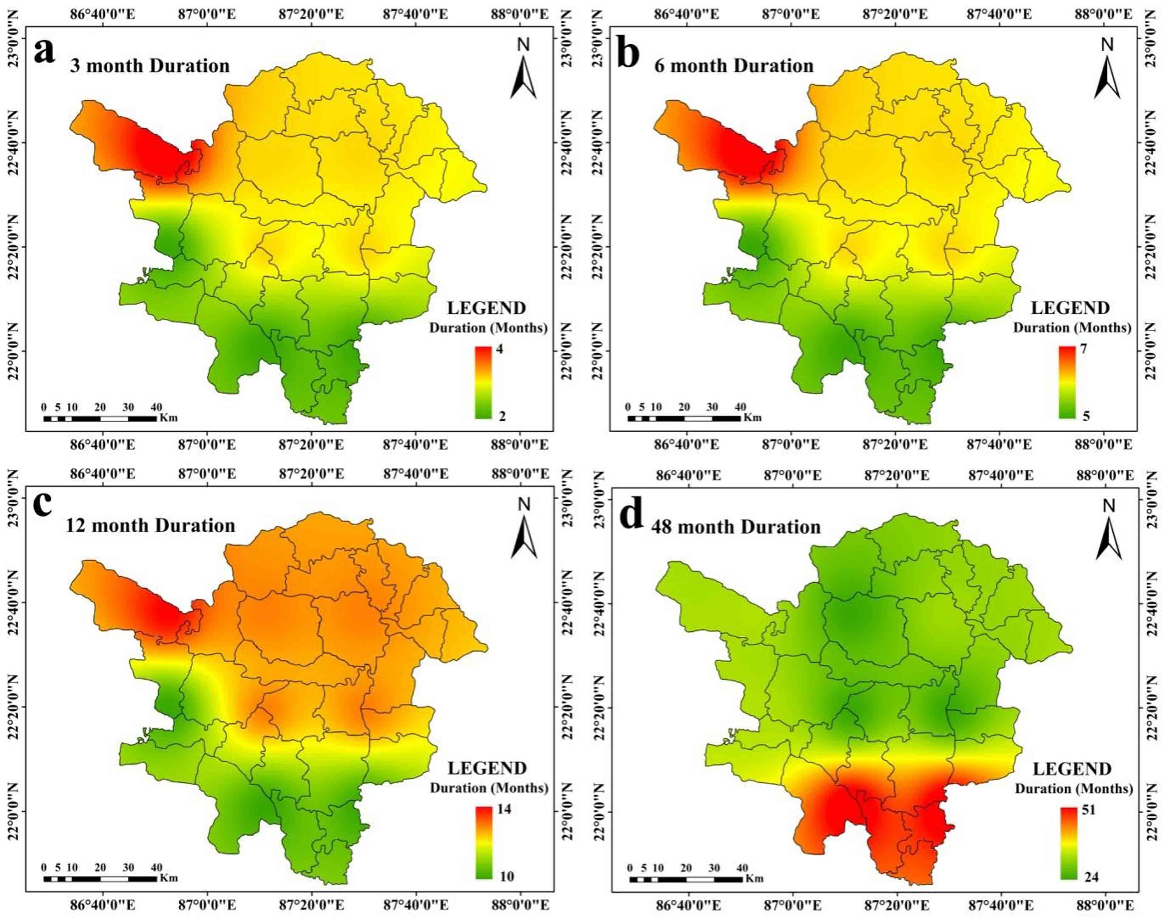
At 48 months’ time step, drought is at the peak, at 220872 (1st Station) and 220875 station (8th Station) with -2.35 SPEI value, which is observed on October 2012 (Table 6). Average drought is also intensified at 220872 (1st Station) and 220875 (8th Station) with -1.49 SPEI value. Drought magnitude is highest at 220872 (1st Station) and 220875 station (8th Station) (-125.63) (Table 7). Average drought duration is also high at 220872 (1st Station) and 220875 station with 14 to 18 months (Figure 6a and Figure 6b). Average drought duration is within 10 to 18 months (Figure 6a-6g). The highest rates of incidence of ES and moderate drought are also seen at stations 220872 (1st Station) and 220875. In the 48 months’ time step, significant negative trend is noticed in 220872 (1st Station), 223872 (2nd Station), 223875 (3rd Station), 226875 (7th Station) and 220875 (8th Station) stations. Other stations are noticed with positive and negative trends of drought which are non-significant in character (Table 6).
Table 6. Station-wise assessment of drought at 48 months
|
Stations |
Peak intensity (PID) |
Peak intensity observed |
Moderate drought occurrence rate |
Extreme to severe (ES) drought occurrence rate |
Average intensity |
Mann-Kendall trend |
Sen's slope |
|
220872 (1st Station) |
-2.35639 |
October-2012 |
18.06 |
14.58 |
-1.49564 |
-0.09* |
-0.99* |
|
223872 (2nd Station) |
-2.21511 |
August-2012 |
6.71 |
2.78 |
-1.44081 |
-0.09* |
-1.18* |
|
223875 (3rd Station) |
-2.21511 |
August-2012 |
6.71 |
2.79 |
-1.44081 |
-0.09* |
-1.18* |
|
226869 (4th Station) |
-1.99327 |
August-2012 |
6.48 |
2.78 |
-1.3773 |
0.03 |
0.07 |
|
223869 (5th Station) |
-1.99327 |
August-2012 |
6.48 |
2.78 |
-1.3773 |
0.03 |
-0.07 |
|
226872 (6th Station) |
-2.21511 |
August-2012 |
6.71 |
2.78 |
-1.44081 |
-0.09 |
1.18 |
|
226875 (7th Station) |
-2.21511 |
August-2012 |
6.71 |
2.79 |
-1.44081 |
-0.09* |
-1.18* |
|
220875(8th Station) |
-2.35639 |
October-2012 |
18.06 |
14.58 |
-1.49564 |
-0.09* |
-0.99* |
*At 0.05 significance level.
Table 7. Drought magnitudes
|
Station Code |
At 3 Months |
At 6 Months |
At 12 Months |
At 48 Months |
|
220872 (1st Station) |
-135.96 |
-129.83 |
-138.13 |
-125.63 |
|
223872 (2nd Station) |
-118.12 |
-119.87 |
-103.37 |
-57.63 |
|
223875 (3rd Station) |
-118.12 |
-119.87 |
-103.37 |
-57.63 |
|
226869 (4th Station) |
-113.82 |
-110.84 |
-96.35 |
-48.21 |
|
223869 (5th Station) |
-113.82 |
-110.84 |
-96.35 |
-48.21 |
|
226872 (6th Station) |
-118.12 |
-119.87 |
-103.36 |
-57.63 |
|
226875 (7th Station) |
-118.12 |
-119.87 |
-103.37 |
-57.63 |
|
220875 (8th Station) |
-135.96 |
-129.84 |
-138.13 |
-125.63 |
*At 0.05 significance level
4.3 Spatial Assessments of Drought
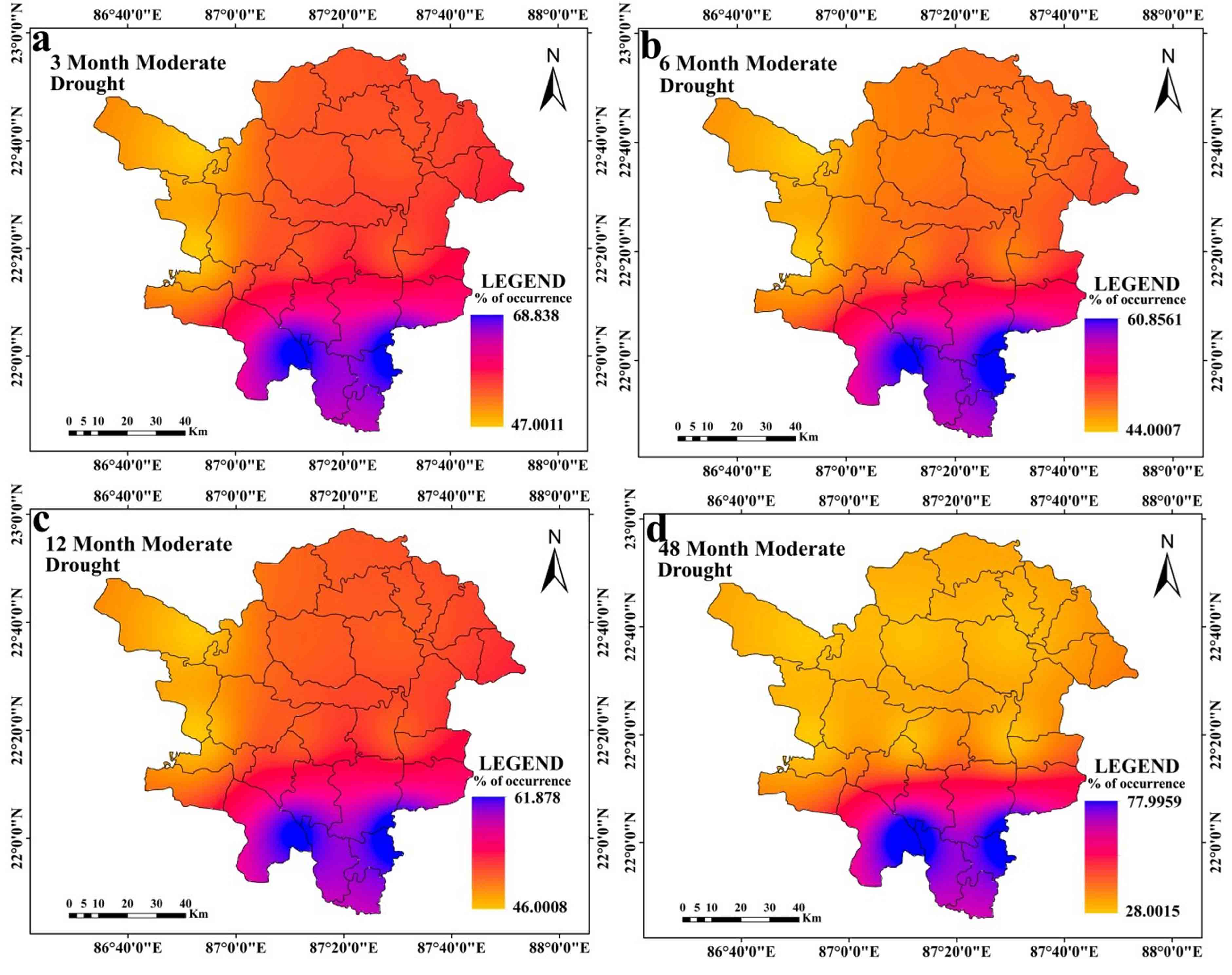
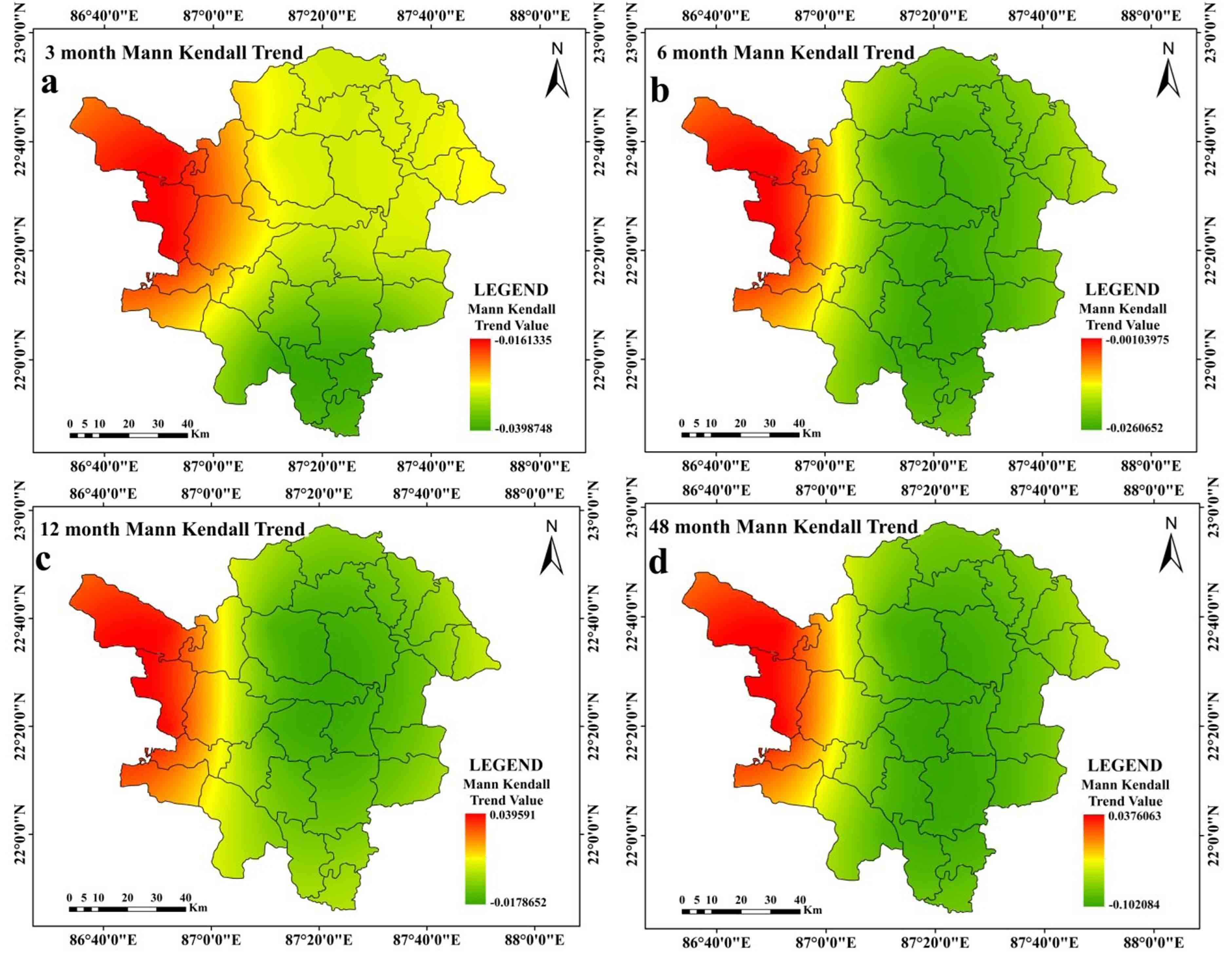
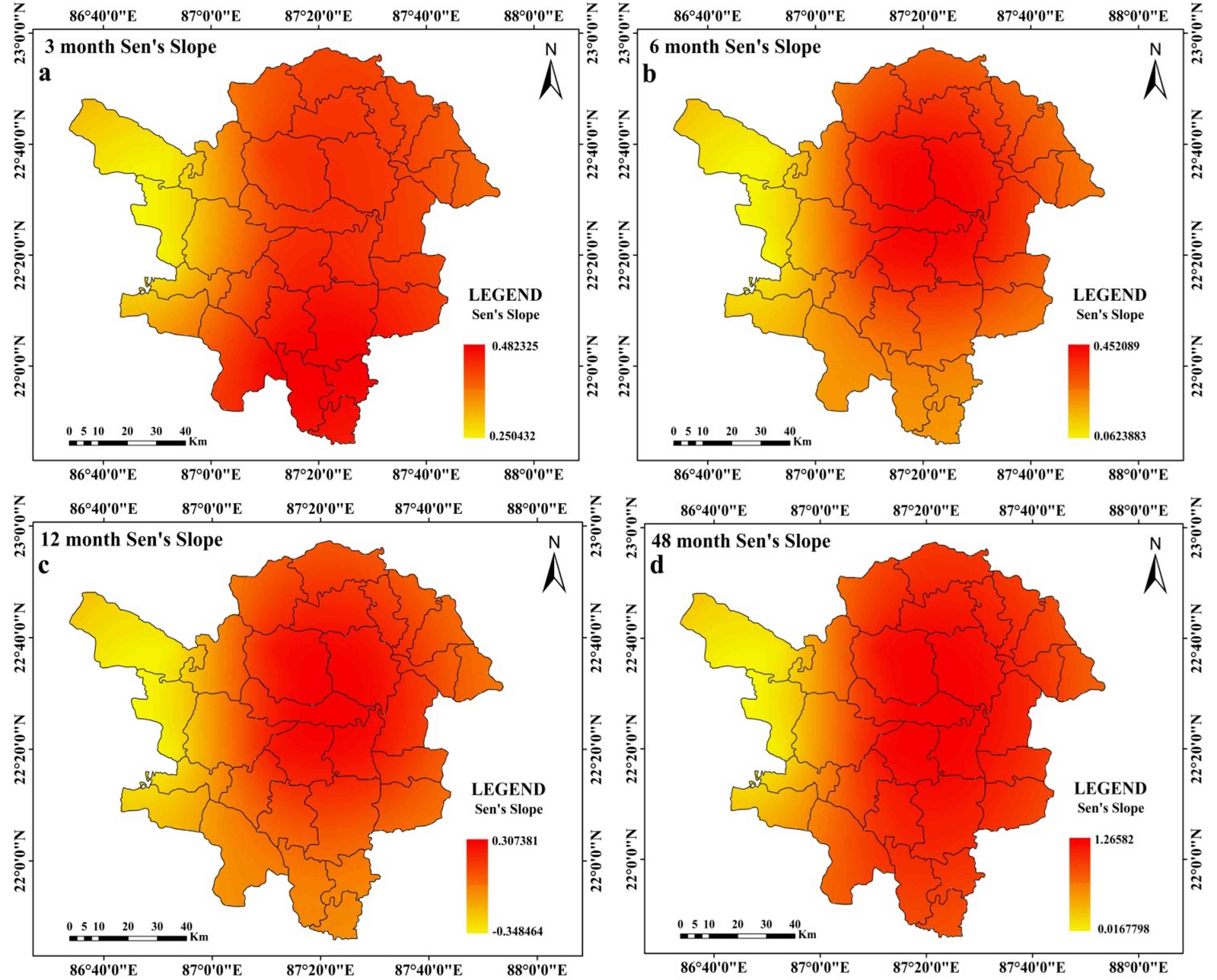
While peak drought is observed in the southern and western portions of the research region at the 12 months time step (Figure 3c), it is at its highest at the 3 months and 6 months time steps in the western portions of the study region. Peak drought moves in the southern parts of the region over a time period of 48 months (Ffigure 3d). At time steps of 3 months, 6 months, and 12 months (Figure 4a, 4b, and 4c, respectively), the average drought in the western parts of the study region gets worse. Southern regions are seen to have greater average drought intensity at a 48-month time step (Figure 4d). Drought is at its’ highest magnitude in southern portions of the study region and this feature is almost similar at all-time steps (Figure 5a-5d). Average drought duration is long in the western parts of the study region for time steps of 3 months, 6 months and 12 months (Figure 6a-6c). Southern regions are seen to have longer average drought durations at 48 months time step (Figure 6d). At 3 months’ time step, western portions of the study area are noticed with highest occurrence rate of ES drought (Figure 7a). At other time steps (6 months, 12 months and 48 months time step) southern portions of the region are noticed with high rate of occurrence of ES drought (Figure 7b, 7c, 7d). At all-time steps, the southern portions are noticed with higher occurrence rate of moderate drought (Figure 8a-8d). At every time steps, negative MK and Sen’s slope value is observed in the western and southwestern portions of the study area (Figure 9a-9d and Figure 10a-10d). Eastern and south-eastern portions are characterized with positive MK and Sen’s slope value (Figure 9a-9d and Figure 10a-10d). The general nature of the region is that as the time step increases, duration of drought starts to increase but intensity, occurrence rate starts to decrease in a significant proportion. Another interesting feature is that drought starts to shift from western portions to southern portions of the study region.
4.4 Assessments of Drought Susceptibility
Zones that are susceptible to drought are evaluated using composite PCA scores (PCA). Here, the first four components are utilized because they account for 80% of the total data. Drought is noted as high, high moderate and moderate at the southern regions of at the 3- and 6-months’ time steps. In the eastern and western halves, respectively; the low, moderate and low categories are present (Figure 11a and 11b). High, high moderate, moderate and low moderate categories predominate in the southern regions at the 12- and 48-months time steps. Remaining portions are noticed with the low drought category (Figure 11c and 11d). In aggregate, low and low moderate categories account for 77.32% of the research area. However, 16.03% of the region is classified as high and high moderate. The remaining regions (6.64%) are classified as being in the moderate drought category (Table 8).
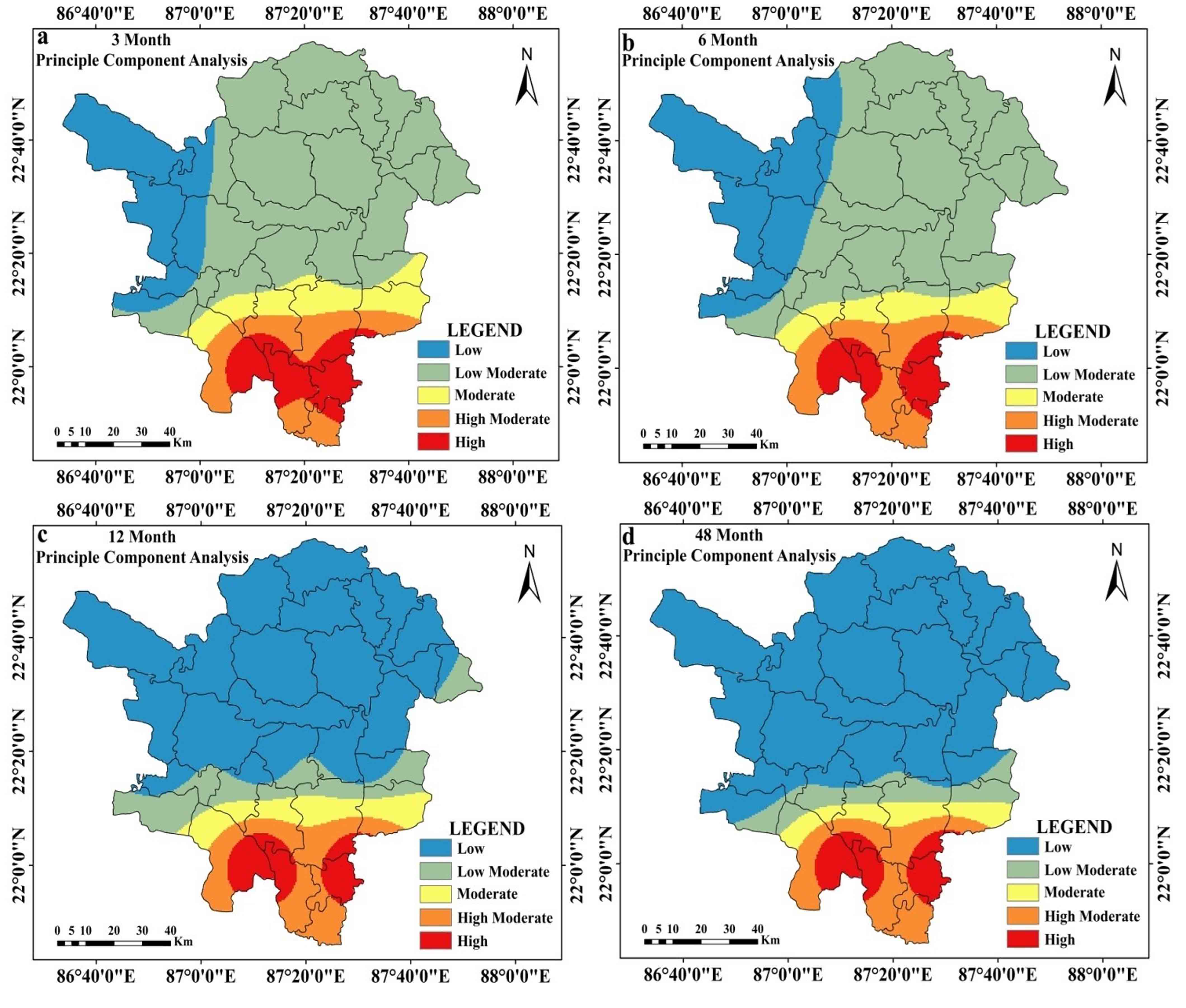
Table 8. Estimated area under drought
|
Categories |
Area (%) |
||||
|
3 Months |
6 Months |
12 Months |
48 Months |
Average |
|
|
Low |
16.81 |
22.99 |
66.53 |
72.69 |
44.75 |
|
Low moderate |
57.36 |
54.02 |
11.42 |
7.50 |
32.57 |
|
Moderate |
8.41 |
6.71 |
6.65 |
4.79 |
6.64 |
|
High moderate |
9.17 |
10.13 |
9.80 |
9.27 |
9.59 |
|
High |
8.26 |
6.16 |
5.60 |
5.75 |
6.44 |
5. Discussion
The trend of drought in India’s Paschim Medinipur District and throughout West Bengal is persistent. Potential causes of this trend might have a tight connection to geo-environmental elements like global climate change (Aind et al., 2022). It shows a recent deterioration in the link between ENSO and the monsoon since the correlation between India's monsoon patterns and ENSO shifted from the year 1990 and achieved its’ peak positivity in the last 10 years (Krishnaswamy et al., 2015). Walker circulation migrate southward as a result of global warming, and these regions exhibit higher surface temperatures more frequently, which is the true explanation of this link (Kundu and Mondal, 2019). Therefore, the drought pattern in the context of Paschim Medinipur cannot be entirely explained by a single ENSO event. Looking at things more broadly, the weakening of the easterly jet stream and the warming of the equatorial ocean are two regional factors that often have an impact on the likelihood for drought to worsen in the southern parts of the Paschim Medinipur district (Ghosh, 2019). The study of drought in these sections is devoted to micro level variability of at eight meteorological stations (Nandi and Sarkar, 2021; Mondal and Sahoo, 2022). Therefore, the impact of ENSO and other events was not evaluated. This research has essentially implicated changes in agricultural property due to the advent of irrigated agriculture, deforestation and expanding urban development. Local level elements include terrain, altitude, gradient, etc. (Kundu and Mondal, 2019). Crystalline bedrock that was formerly a part of a granitic environment and was sparsely covered by a weathered mantle may be found in the Paschim Medinipur area (Ghosh and Guchhait, 2020). These sections contain scattered shallow rupture zones that cannot store adequate groundwater due to their disrupted nature (Das et al., 2022). The worn fracture zone limits the quantity of groundwater in certain sections of the study area (Upadhayay et al., 2019). Secondary porosity or the formation of a thick profile in the porous material, is seen in the fracture zone (Nag and Ghosh, 2013). The secondary porosity is apparent as a result of the ongoing weathering of the hard, cemented rock. Secondary porosity, or the formation of a thick profile in the porous material, is seen in the fracture zone.
6. Conclusion
In this study, drought was assessed spatiotemporally at 3 months, 6 months, 12 months and 48 months time step. Peak intensity, average drought intensity, magnitude, extreme to severe and moderate drought occurrence rate and trend of drought were portrayed using visual interpretative maps and statistical assessment. At the end, the drought prone zones were demarcated by Principal Component Analysis, which was estimated using above mentioned parameters at several time steps. At every time steps, drought was fatal in the southern and southwestern portions of Paschim Medinipur. The remaining portions of Paschim Medinipur were at near normal of wet condition, which was indicated as low moderate and low category in figure 14. Overall 16% area was under high drought prone region, whereas 66% area was under low drought prone zone. The remaining portions of the region were under moderate drought proneness. It is interesting to note that as the time step increases, the percentage share of low and low moderate drought prone area increases and high and high drought prone area decreases in a significant proportion.
This study is intriguing and special since it emphasises the station-by-station micro level assessment of drought over a number of time periods. This study is useful for implementation since it allows for the quick identification and monitoring of many drought-related factors. The result of this research may help Medinipur’s water management infrastructure and planning. The observed drought risk events, both spatially and temporally, show a possible risk to agrarian agriculture techniques, which are common in the current study area. Drought will result in less production if prompt action is not done, which will ultimately have an impact on farmers’ financial situation. Therefore, examination of various drought evaluation indicators is crucial for managing food security, planning at the local level and early warning measures. The study is a crucial step in improving the area’s drought risk management plan.
Conflict of interest
No conflict of interest exists to publish the article.
Acknowledgements
We are very much thankful to Editors and Reviewers who has helped us to improve the manuscript time to time.
Abbreviations
Dp: Drought Evaluation Parameters; FD: Frequency of Drought; ID: Drought Intensity; MD:Magnitude of Drought; MID: Average Drought Intensity; PCA: Principal Component Analysis; SPEI: Standardized Precipitation Evapotranspiration Index.
Article information
- Received
- 20 Oct 2022
- Revised
- 3 Dec 2022
- Accepted
- 4 Dec 2022
- Published
- 18 Dec 2022
- Handling editor
- Dr. Vasant Wagh
- Licence
- CC BY-NC-ND 4.0
- Journal
- Hydrospatial Analysis, ISSN 2582-2969
References
-
Abbasi, A., Khalili, K., Behmanesh, J. and Shirzad, A., 2019. Drought monitoring and prediction using SPEI index and gene expression programming model in the west of Urmia Lake. Theoretical and Applied Climatology, 138(1), 553-567.
Crossref -
Abeysingha, N. S. and Rajapaksha, U. R. L. N., 2020. SPI-based spatiotemporal drought over Sri Lanka. Advances in Meteorology, 2020, 1-10.
Crossref -
Abramowitz, M. and Stegun, I. A. (Eds.), 1964. Handbook of mathematical functions with formulas, graphs, and mathematical tables, 55. US Government printing office.
-
Aind, D. A., Malakar, P., Sarkar, S. and Mukherjee, A., 2022. Controls on groundwater fluoride contamination in eastern parts of India: Insights from Unsaturated zone fluoride profiles and AI-based modeling. Water, 14(20), 3220.
Crossref -
Alam, N. M., Sharma, G. C., Moreira, E., Jana, C., Mishra, P. K., Sharma, N. K. and Mandal, D., 2017. Evaluation of drought using SPEI drought class transitions and log-linear models for different agro-ecological regions of India. Physics and Chemistry of the Earth, Parts A/B/C, 100, 31-43.
Crossref -
Beguería, S., Vicente-Serrano, S. M., Reig, F. and Latorre, B., 2013. Standardized precipitation evapotranspiration index (SPEI) revisited: parameter fitting, evapotranspiration models, tools, datasets and drought monitoring. International Journal of Climatology, 34(10), 3001-3023.
Crossref -
Bera, B., Shit, P. K., Sengupta, N., Saha, S. and Bhattacharjee, S., 2021. Trends and variability of drought in the extended part of Chhota Nagpur plateau (Singbhum Protocontinent), India applying SPI and SPEI indices. Environmental Challenges, 5, 100310.
Crossref -
Bezdan, J., Bezdan, A., Blagojević, B., Mesaroš, M., Pejić, B., Vranešević, M., Pavić, D. and Nikolić-Đorić, E., 2019. SPEI-based approach to agricultural drought monitoring in Vojvodina region. Water, 11(7), 1481.
Crossref -
Bhave, A.G., Mishra, A. and Groot, A., 2013. Sub-basin scale characterization of climate change vulnerability, impacts and adaptation in an Indian River basin. Reg. Environ Change 13(5), 1087-1098.
Crossref -
Cai, W., Zhang, Y., Chen, Q. and Yao, Y., 2015. Spatial patterns and temporal variability of drought in Beijing-Tianjin-Hebei metropolitan areas in China. Adv Meteorol., 1-14.
Crossref -
Caloiero, T., Veltri, S., Caloiero, P. and Frustaci, F., 2018. Drought Analysis in Europe and in the Mediterranean Basin Using the Standardized Precipitation Index. Water, 10(8), 1043.
Crossref -
Chanda, K., Maity, R., Sharma, A. and Mehrotra, R., 2014. Spatio-temporal variation of long‐term drought propensity through reliability‐resilience‐vulnerability based Drought Management Index. Water Resources Research, 50(10), 7662-7676.
Crossref -
Chhajer, V., Prabhakar, S. and Ram Chandra, P., 2015 Development of index to assess drought conditions using geospatial data a case study of Jaisalmer District, Rajasthan, India. Geoinformatica Polonica, 14(1), 29-39.
Crossref -
CRED [Centre for Research on the Epidemiology of Disasters], 2016. Country profile of natural disasters, EM-DAT: The International Disaster Database.
-
Dai, A., 2011. Drought under global warming: A review. Wiley Interdisciplinary Reviews: Climate Change, 2(1), 45-65.
Crossref -
Das, P., Maya, K. and Padmalal, D., 2022. Hydrogeochemistry of the Indian thermal springs: Current status. Earth Science Reviews, 224, 103890.
Crossref -
Datta, P. and Das, S., 2019. Analysis of long-term precipitation changes in West Bengal, India: An approach to detect monotonic trends influenced by autocorrelations. Dynamics of Atmospheres and Oceans, 88, 1011118.
Crossref -
Demšar, U., Harris, P., Brunsdon, C., Fotheringham, A.S. and McLoone, S., 2013. Principal component analysis on spatial data: An overview. Annals of the Association of American Geographers, 103(1), 106-128.
Crossref -
Dile, Y. T. and Srinivasan, R., 2014. Evaluation of CFSR Climate Data for Hydrologic Prediction in Data‐Scarce Watersheds: an Application In The Blue Nile River Basin. JAWRA, 50(5), 1226-1241.
Crossref -
Dinpashoh, Y., Fakheri-Fard, A., Moghaddam, M., Jahanbakhsh, S. and Mirnia, M., 2004. Selection of variables for the purpose of regionalization of Iran's precipitation climate using multivariate methods. J. Hydrol., 297(1-4), 109-123.
Crossref -
Dogan, S., Berktay, A. and Singh, V. P., 2012. Comparison of multi-monthly rainfall-based drought severity indices, with application to semi-arid Konya closed basin, Turkey. Journal of Hydrology, 470-471, 255-268.
Crossref -
Dracup, J. A., Lee, K. S. and Paulson Jr., E. G., 1980. On the definition of droughts. Water Resources Research. 16 (2), 297-302.
Crossref -
Dupigny-Giroux, L. A., 2001. Towards characterizing and planning for drought in Vermont: Part-I: A climatological perspective. Journal of the American Water Resources Association 37 (3), 505-525.
Crossref -
Durdu, Ö. F., 2010. Application of linear stochastic models for drought forecasting in the Büyük Menderes river basin, western Turkey. Stoch. Env. Res. Risk. Ass., 24(8), 1145-1162.
Crossref -
Ghosh, K. G., 2018. Analysis of rainfall trends and its spatial patterns during the last century over the Gangetic West Bengal, Eastern India. Journal of Geovisualization and Spatial Analysis, 2(2), 1-18.
Crossref -
Ghosh, K. G., 2019. Spatial and temporal appraisal of drought jeopardy over the Gangetic West Bengal, eastern India. Geoenvironmental Disasters, 6(1), 1-21.
Crossref -
Ghosh, S. and Guchhait, S. K., 2020. Laterites of the Bengal Basin: Characterization, geochronology and evolution (p. Basel). Switzerland: Springer.
Crossref -
Guo, E., Liu, X., Zhang, J., Wang, Y., Wang, C., Wang, R. and Li, D., 2017. Assessing spatiotemporal variation of drought and its impact on maize yield in Northeast China. Journal of Hydrology, 553, 231-247.
Crossref -
Gupta, A. K., Tyagi, P., and Sehgal, V. K., 2011. Drought disaster challenges and mitigation in India: Strategic appraisal. Current Science. 100(12), 1795-1806.
-
Gupta, A., Kamble, T. and Machiwal, D., 2017. Comparison of ordinary and Bayesian kriging techniques in depicting rainfall variability in arid and semi-arid regions of north-west India. Environmental Earth Sciences, 76(15), 1-16.
Crossref -
Halder, S., Roy, M. B. and Roy, P. K., 2020. Analysis of groundwater level trend and groundwater drought using Standard Groundwater Level Index: A case study of an eastern river basin of West Bengal, India. SN Applied Sciences, 2(3), 1-24.
Crossref -
IPCC [Intergovernmental Panel on Climate Change], 2007. Climate change 2007: The physical science basis. In Contribution of working group I to the fourth assessment report of the intergovernmental panel on climate change, ed. S. Solomon, D. Quin, M. Manning, X. Chen, M. Marquis, K.B. Averyt, H.L. Tignor, and M. Miller, 1-996. Cambridge: Cambridge University Press.
-
Jolliffe, I. T., 2002. Principal component analysis for special types of data, 338-372. Springer, New York.
-
Kamble, M. V., Ghosh, K., Rajeevan, M. and Samui, R. P., 2010. Drought monitoring over India through normalized difference vegetation index (NDVI). Mausam 61, 537-546.
-
Kar, B., and Saha, J., 2012. Analysis of meteorological drought: The scenario of West Bengal. Indian J. Spatial Sci., 3(2), 1-11.
-
Karavitis, C. A., Alexandris, S., Tsesmelis, D. E. and Athanasopoulos, G., 2011. Application of the Standardized Precipitation Index (SPI) in Greece. Water, 3(3), 787-805.
Crossref -
Kendall, M. G., 1975. Rank Correlation Methods, Griffin, London.
-
Khan J. H., Hassan T. and Shamsad, 2011. Socio economic causes of rural urban migration in India. Asia-Pacific Journal of Social Sciences. 138-158.
-
Krishnaswamy, J., Vaidyanathan, S., Rajagopalan, B., Bonell, M., Sankaran, M., Bhalla, R. S. and Badiger, S., 2015. Non-stationary and non-linear influence of ENSO and Indian Ocean Dipole on the variability of Indian monsoon rainfall and extreme rain events. Climate Dynamics, 45(1), 175-184.
Crossref -
Kundu, S. K., and Mondal, T. K., 2019. Analysis of long-term rainfall trends and change point in West Bengal, India. Theoretical and Applied Climatology, 138(3), 1647-1666.
Crossref -
Kwon, M., Kwon, H., and Han, D., 2019. Spatio‐temporal drought patterns of multiple drought indices based on precipitation and soil moisture: A case study in South Korea. International Journal of Climatology.
Crossref -
Liu, X., Wang, S., Zhou, Y., Wang, F., Li, W. and Liu, W., 2015. Regionalization and spatiotemporal variation of drought in China based on standardized precipitation evapotranspiration index (1961-2013). Advances in Meteorology.
Crossref -
Lohar, D., and Pal, B., 1995. The effect of irrigation on pre-monsoon season precipitation over south West Bengal, India. J. Climate, 8(10), 2567-2570.
Crossref -
Mann, H. B., 1945. Nonparametric tests against trend. Econometrica: Journal of the Econometric Society, 245-259.
Crossref -
Measho, S., Chen, B., Trisurat, Y., Pellikka, P., Guo, L., Arunyawat, S., and Yemane, T., 2019. Spatio-temporal analysis of vegetation dynamics as a response to climate variability and drought patterns in the Semiarid Region, Eritrea. Remote Sensing, 11(6), 724.
Crossref -
Mirabbasi, R., Anagnostou, E. N., Fakheri-Fard, A., Dinpashoh, Y. and Eslamian, S., 2013. Analysis of meteorological drought in northwest Iran using the joint deficit index. Journal of Hydrology, 492, 35-48.
Crossref -
Mishra, A. K., and Singh, V. P., 2011. Drought modeling- A review. J. Hydrol, 403(1-2), 157-175.
Crossref -
Mishra, M. K., Khare, N., and Agrawal, A. B., 2015. Scenario analysis of the CO2 emissions reduction potential through clean coal technology in India's power sector: 2014-2050. Energy Strategy Reviews, 7, 29-38.
Crossref -
Mondal, B. K., and Sahoo, S., 2022. Evaluation of spatiotemporal dynamics of water storage changes at block level for sustainable water management in Howrah District of West Bengal. Environment, Development and Sustainability, 24(7), 9519-9568.
Crossref -
Musei, S. K., Nyaga, J. M., and Dubow, A. Z., 2021. SPEI-based spatial and temporal evaluation of drought in Somalia. Journal of Arid Environments, 184, 104296.
Crossref -
Nag, S. K., and Ghosh, P., 2013. Delineation of groundwater potential zone in Chhatna Block, Bankura District, West Bengal, India using remote sensing and GIS techniques. Environmental Earth Sciences, 70(5), 2115-2127.
Crossref -
Nandi, D., and Sarkar, S., 2021. Upstream effects of dam on livelihoods of agriculture-dependent communities: A micro-level study of Itamara mouza in Hirbandh CD block, Bankura District, West Bengal (India). Journal of Cleaner Production, 313, 127893.
Crossref -
Nikzad Tehrani, E., Sahour, H. and Booij, M. J., 2019. Trend analysis of hydro-climatic variables in the north of Iran. Theoretical and Applied Climatology, 136(1), 85-97.
Crossref -
NRC [National Research Council] 2010. Adapting to the impacts of climate change: America’s climate choices. Washington, DC: National Academies Press.
-
Sadeghi, S. H., and Hazbavi, Z., 2017. Spatiotemporal variation of watershed health propensity through reliability-resilience-vulnerability based drought index (case study: Shazand Watershed in Iran). Science of The Total Environment, 587, 168-176.
Crossref -
Saharwardi, M. S., and Kumar, P., 2022. Future drought changes and associated uncertainty over the homogenous regions of India: A multimodel approach. International Journal of Climatology, 42(1), 652-670.
Crossref -
Sen, P. K., 1968. Estimates of the regression coefficient based on Kendall’s tau. J Am Stat Assoc., 63(324), 1379-1389.
-
Shadeed, S., 2013. Spatio-temporal drought analysis in arid and semi-arid regions: A case study from Palestine. Arabian Journal for Science and Engineering, 38(9), 2303-2313.
Crossref -
Sommerlot, A. R., 2017. Coupling Physical and Machine Learning Models with High Resolution Information Transfer and Rapid Update Frameworks for Environmental Applications (Doctoral dissertation, Virginia Tech). Accessed 15 April 2020.
-
Sonmez, F. K., Komuscu, A. U., Erkan, A. and Turgu. E., 2005. An analysis of spatial and temporal dimension of drought vulnerability in Turkey using the standardized precipitation index. Natural Hazards. 35(2), 243-264.
Crossref -
Spinoni, J., Naumann, G., Carrao, H., Barbosa, P. and Vogt, J., 2014. World drought frequency, duration, and severity for 1951-2010. International Journal of Climatology, 34(8), 2792-2804.
Crossref -
Stagge, J. H., Tallaksen, L. M., Gudmundsson, L., Van Loon, A. F. and Stahl, K., 2015. Candidate distributions for climatological drought indices (SPI and SPEI). International Journal of Climatology, 35(13), 4027-4040.
Crossref -
Svoboda, M. and Fuchs, B., 2016. Handbook of drought indicators and indices. National Drought Mitigation Center, Lincoln, NE. Accessed: 23rd April 2020.
-
Tabari, H., Somee, B. S. and Zadeh, M. R., 2011. Testing for long-term trends in climatic variables in Iran. Atmos. Res., 100(1), 132-140.
Crossref -
Tefera, A. S., Ayoade, J. O. and Bello, N. J., 2019. Comparative analyses of SPI and SPEI as drought assessment tools in Tigray Region, Northern Ethiopia. SN Applied Science, 1, 1265.
Crossref -
Theil, H., 1950. A rank invariant method of linear and polynomial regression analysis, part 3. Netherlands Akademie van Wettenschappen. Proceedings, 53, 1397-1412.
-
Thomas, T., Nayak, P. C., and Ghosh, N. C., 2015. Spatiotemporal analysis of drought characteristics in the Bundelkhand region of Central India using the standardized precipitation index. Journal of Hydrologic Engineering, 20(11), 05015004.
Crossref -
Thompson, S., 1999. Hydrology for water management, 476. Rotterdam, The Netherlands: AA Balkema Publ.
-
Thornthwaite, C. W., 1948. An approach toward a rational classification of climate. Geogr. Rev., 38, 55-94.
-
Tong, S., Lai, Q., Zhang, J., Bao, Y., Lusi, A., Ma, Q., Li, X. and Zhang, F., 2018. Spatiotemporal drought variability on the Mongolian Plateau from 1980-2014 based on the SPEI-PM, intensity analysis and Hurst exponent. Science of the Total Environment, 615, 1557-1565.
Crossref -
Trenberth, K. E., Dai, A., Schrier, G., Jones, P. D., Barichivich, J., Briffa, K. R. and Sheffield, J., 2014. Global warming and changes in drought. Nature Climate Change 4, 17-22.
Crossref -
Upadhayay, U., Kumar, N., Kumar, R. and Kumari, P., 2019. Hydro-geological status of the core and buffer zone of Beekay Steel Industries Limited, Adityapur Industrial Area, Saraikela, Kharsawan, Jharkhand. In Wastewater Reuse and Watershed Management, 219-246, Apple Academic Press.
-
Vicente-Serrano, S. M., Beguería, S. and López-Moreno, J. I., 2010. A Multiscalar Drought Index Sensitive to Global Warming: The standardized precipitation evapotranspiration index. Journal of Climate, 23(7), 1696-1718.
Crossref -
Wable, P. S., Jha, M. K. and Shekhar, A., 2019. Comparison of drought indices in a semi-arid river basin of India. Water Resources Management, 33(1), 75-102.
Crossref -
Wang, F., Wang, Z., Yang, H. and Zhao, Y., 2018. Study of the temporal and spatial patterns of drought in the Yellow River basin based on SPEI. Science China Earth Sciences, 61(8), 1098-1111.
Crossref -
Wang, Q., Shi, P., Lei, T., Geng, G., Liu, J., Mo, X., Li, X., Zhou, H. and Wu, J., 2015. The alleviating trend of drought in the Huang‐Huai‐Hai Plain of China based on the daily SPEI. International Journal of Climatology, 35(13), 3760-3769.
Crossref -
White, M. J., Gambone, M., Haney, E., Arnold, J. and Gao, J., 2017. Development of a station based climate database for SWAT and APEX Assessments in the US. Water, 9(6), 437.
Crossref -
Xu, D., Zhang, Q., Ding, Y. and Zhang, D., 2022. Application of a hybrid ARIMA-LSTM model based on the SPEI for drought forecasting. Environmental Science and Pollution Research, 29(3), 4128-4144.
Crossref -
Yan, H., Wang, S. Q., Wang, J. B., Lu, H. Q., Guo, A. H., Zhu, Z. C., Myneni, R. B. and Shugart, H. H., 2016. Assessing spatiotemporal variation of drought in China and its impact on agriculture during 1982-2011 by using PDSI indices and agriculture drought survey data. Journal of Geophysical Research: Atmospheres, 121(5), 2283-2298.
Crossref -
Yang, C., Tuo, Y., Ma, J. and Zhang, D., 2019. Spatial and temporal evolution characteristics of drought in Yunnan Province from 1969 to 2018 based on SPI/SPEI. Water, Air and Soil Pollution, 230(11), 1-13.
Crossref -
Yang, M., Yan, D., Yu, Y. and Yang, Z., 2016. SPEI-based spatiotemporal analysis of drought in Haihe River Basin from 1961 to 2010. Advances in Meteorology.
Crossref -
Yu, M., Xi, C., Li, L., Bao, A., and Paix, M. J., 2011. Streamflow simulation by SWAT using different precipitation sources in large arid basins with scarce raingauges. Water Resour. Manage. 25, 2669.
Crossref -
Zarch, M. A. A., Sivakumar, B., and Sharma, A., 2015. Droughts in a warming climate: A global assessment of standardized precipitation index (SPI) and reconnaissance drought index (RDI). J. Hydrol., 526, 183-195.
Crossref -
Zarei, A. R. and Moghimi, M. M., 2019. Modified version for SPEI to evaluate and modeling the agricultural drought severity. International Journal of Biometeorology, 63(7), 911-925.
Crossref -
Zhang, L. and Zhou, T., 2015. Drought over East Asia: A review. J. Climate, 28(8), 3375-3399.
Crossref -
Zou, H., Hastie, T. and Tibshirani, R., 2006. Sparse Principal Component Analysis. J. Comput. Graph. Stat., 15(2), 265-286.
Crossref